 Maria Amaya
 Ayden Baran2
 John C. Little
94% of researchers rate our articles as excellent or good
Learn more about the work of our research integrity team to safeguard the quality of each article we publish.
Find out more
CONCEPTUAL ANALYSIS article
Front. Water, 03 June 2021
Sec. Water and Human Systems
Volume 3 - 2021 | https://doi.org/10.3389/frwa.2021.681553
This article is part of the Research TopicWater Resources and Human Behavior: Analysis and Modeling of Coupled Water-Human Systems Feedbacks and CoevolutionView all 4 articles
To capture the interactions between hydrologic and economic systems necessary for modeling water quality at a sufficient level of spatial detail, we have designed a modular framework that couples an economic model with a watershed model. To represent the economic system, the Rectangular Choice-of-Technology (RCOT) model was used because it represents both the physical and monetary aspects of economic activities and, unlike traditional input-output or general equilibrium models, it can optimize choices among operational technologies in addition to the amount and location of production. For the first implementation of this modeling framework, RCOT is coupled with a watershed model, Hydrological Simulation Program-Fortran (HSPF), which was calibrated to represent Cedar Run Watershed in northern Virginia. This framework was used to analyze eight scenarios related to the expansion of agricultural activity in Fauquier County. The database for RCOT used county-level input-output data representative of the region in 2012. Thus, when crop farming was expanded to fully utilize the farmland available in the watershed, the nitrogen concentration at the outflow of the watershed increased from 0.6 to 4.3 mg/L. However, when RCOT could select between a standard and a more nitrogen-efficient management practice, the outflow nitrogen concentration only increased to 2.6 mg/L because RCOT selected the more resource-efficient practice. Building on this modular framework, future work will involve designing more realistic scenarios that can test policy options and regional planning decisions in a wide range of watersheds.
The engineering and economic disciplines have historically maintained an association since economic costs and benefits are important concerns when designing, building, and maintaining infrastructure. However, the role of economic principles has begun to expand in engineering, particularly in the field of water resources engineering where concerns of water availability and quality have become more deeply intertwined with socio-economic impacts. Applying economic concepts in water engineering can enhance insight into forecasting water demand, evaluating engineering designs, negotiating water policy, as well as understanding water management concerns across local, regional, and global scales (Lund et al., 2006). Water is a resource used both in production activities and directly by consumers, but it also serves as a receptor for the pollution byproducts of production and consumption. Therefore, while water must be utilized for economic purposes, the impact of economic use on water quantity and quality must be simultaneously considered (Brouwer and Hofkes, 2008).
Hydro-economic modeling has been developed by hydrologists and engineers to represent the interactions between hydrologic and economic systems. The integration process may include considering multiple disciplinary views to a problem, linking different system or process models, harmonizing different scales of process operation, assessing the effects of management options on various economic, and environmental issues, or any combination of these concepts (Kelly et al., 2013). Typically, hydro-economic models combine water quantity models, water allocation models, or water quality models with economic variables of supply and demand on the basis that water systems carry economic value. However, several challenges can occur when trying to combine water and economic systems. First, hydrologic models usually are spatially defined by watersheds or basins while economic models are typically defined by administrative boundaries. Additionally, hydrological models can be temporally defined from hours to months while typical economic models are temporally defined in years or longer. Furthermore, hydrologic models are typically based on theories or empirical relationships among variables while economic models often use statistical inference to establish relationships among variables (McKitrick, 1998; Brouwer and Hofkes, 2008). These challenges can be addressed differently depending on the modeling approach being utilized and the application of the modeling framework. Three approaches used for hydro-economic modeling include the holistic, computable general equilibrium (CGE), and modular approaches (Brouwer and Hofkes, 2008). Each approach is examined in more detail in the following sub-sections.
The holistic modeling approach incorporates the hydrological and economic components of a region into a single integrated software package. As a result, all information is transferred internally within the model and data transformation is not a primary concern. On the other hand, both the hydrological and economic components must be represented by a single solver, and thus each component must be effectively simplified to minimize complexities within that solver (Cai et al., 2003; Brouwer and Hofkes, 2008). The holistic modeling approach has been applied in multiple case studies, including one in the Maipo River basin in Chile (Cai et al., 2008) and several located in Spain (Pulido-Velazquez et al., 2008; Kahil et al., 2016; Escriva-Bou et al., 2017). This approach is typically characterized by a model being developed to simulate hydrologic and economic relationships by presenting the basin as a linked network of supply nodes, such as reservoirs and rivers, and demand nodes representing irrigation, municipal, and industrial entities. Each source node has an associated water balance or storage operation while the demand sites account for short-term economic costs and benefits (Cai et al., 2008; Harou et al., 2009). These holistic models can provide insight into concerns of hydrologic stress that may result from economic productivity, but they have historically lacked sectoral detail or comprehensive representation of a whole economy (Brouwer and Hofkes, 2008).
Traditionally, the holistic approach tends to focus on a comprehensive hydrological system with some extension to economic variables. However, because this approach lacks a detailed economic system, CGE models have been employed in frameworks that integrate hydrological and economic systems. There have been multiple applications of the CGE approach in integrated hydro-economic analysis, such as in an analysis of China's whole economy (Jiang et al., 2014) as well as in more recent case studies (Kahsay et al., 2019; Knowling et al., 2020). These models are economic models capable of representing price-dependent market interactions and can be extended to assess water policy. While this approach can effectively depict economy-wide impacts, it lacks intricate detail in representing hydrological processes (Bohringer and Loschel, 2006; Brouwer and Hofkes, 2008). Furthermore, CGE models may be useful at depicting how a whole economy is impacted by changes in watershed conditions, but hydrologic variables must be transformed into monetary values to be incorporated into these models (Zhang, 2013).
While CGE models have been promoted as an approach to evaluate the interactions between economic and hydrological systems, several shortcomings have been identified regarding the utilization of these models for broader sustainability assessment, which are fully detailed in Scrieciu (2007) and summarized here. First, the economic theory employed in CGE models places great emphasis on the role of market interactions in addressing environmental issues. CGE models also operate using the mainstream theory that behavior is driven by the maximization of personal utility as represented by consumption, which excludes other drivers of human behavior (Zhang, 2013). Additionally, CGE models may be unsuitable for representing changing economies since they have limitations in presenting transitions in technology that can occur because of the implementation of environmental policy. Finally, CGE models alone are not able to adequately capture the localized impacts of large-scale environmental problems. Therefore, an economic model with more sectoral and spatial detail may be better suited for assessing the economic system and its interactions with an environmental system. Furthermore, a model capable of representing the economic components with adequate complexity, coupled with other independently constructed models, could provide a more comprehensive assessment than solely relying on a CGE modeling framework where environmental variables must conform to the underlying principles of CGE models (Scrieciu, 2007).
When applying the modular approach, hydrological and economic models are loosely connected and output data from one model is used as input data for the other (Brouwer and Hofkes, 2008). The modular approach allows for the use of established models and thus enables innovation in new conceptual integration rather than building a simplified model as is the case when applying the holistic modeling approach. However, the data must be correctly transformed for information to be transferred between each model (Cai et al., 2003; Harou et al., 2009), but it has been successfully implemented in several past studies (e.g., Esteve et al., 2015).
Since the modular approach allows for the use of independent models, input-output (I-O) economic models, which are part of an alternative modeling tradition to CGE models, may be used to represent the economic system within the modeling framework. These models provide sectoral details of a regional economy and can capture the inter-sectoral flow of goods among these economic sectors. Furthermore, I-O models can calculate factor quantities, including natural resources, used by each sector and can represent economic demand in physical or monetary units. On the other hand, these models do not typically capture the spatial distribution of these quantities (Harou et al., 2009). However, Jonkman et al. (2008), designed a modular framework to analyze the Netherlands' entire economy and a geographic information system (GIS) was used to spatially transform data so that it could be transferred between a hydrological model and an I-O model Thus, spatial detail is feasible for I-O models.
In general, I-O models are sufficient to use in the modular approach to hydro-economic modeling, but specifically, constrained optimization I-O models are the most suitable alternative to CGE models in representing an economic system within a hydrologic-economic framework. The World Trade Model (WTM) and Rectangular Choice-of-Technology (RCOT) models are recent extensions to this family of models. WTM was developed as a linear programming model that selects among choices of geographic locations (Duchin, 2005). Similarly, RCOT is an input-output linear programming model that, unlike the traditional input-output model or CGE models, endogenously considers choices among operational technologies based on constraints to minimize use of factors of production, which effectively represents human behavior in response to changing environmental conditions (Duchin and Levine, 2011). Since WTM and RCOT are based on the same economic logic, the two models can be easily integrated so that the choices of both alternative technologies and of the spatial location of production may be considered (Duchin and Levine, 2011, 2012). The WTM and RCOT models can represent both the physical and monetary aspects of economic activities. Furthermore, these models can clearly represent the physical availability of water as well as its corresponding cost and price.
The WTM/RCOT model was used in a case study to evaluate water withdrawal policies and their economic implications for the different regions of Mexico (Lopez-Morales and Duchin, 2015). More recently, RCOT has been used to represent the generation, treatment, and discharge of wastewater within the regional economy of Mexico City. In that case study, the choice of technology mechanism within RCOT was used to select between alternate wastewater infrastructure that may be utilized to alleviate overexploitation of natural water sources (Lopez-Morales and Rodriguez-Tapia, 2019). There is a direct interdependence between availability of water and its subsequent quantity and cost for economic activities. As a result, the choice selection among specific technologies available to different economic sectors can change and ultimately affect prices of goods. Thus, this model represents the quantity of inputs required by an economic sector to produce a unit of its output using the technologies in place, which makes it a structural model based on causal relationships rather than a model based on statistical inference. Therefore, RCOT has the necessary complexity to represent the economic system and the use of natural resources within that system as well as the compatibility to be coupled with an independent hydrologic model in a modular framework.
In this paper, we describe a modular framework designed to capture the interactions between a watershed and an economic system that lies within it. RCOT was used to represent the economic system while an HSPF model was used to represent the watershed system. The novelty of this framework lies both in the utilization of RCOT and in the relationship between the two models. RCOT is a regional-scale model and can represent an entire economy with adequate sectoral detail, which typically is lacking in the holistic modeling approach. Additionally, its ability to select among choices in production locations and technologies provides realism in terms of representing human decisions amidst changing economies as well as providing some spatial detail, which has historically been missing from economy-wide models. Furthermore, because RCOT can represent the economy in terms of physical phenomena, this framework can capture how changes in economic activity will alter the physical conditions within the local watershed and how these changes within the watershed in turn limit the economic activity that can occur, which results in a framework that is more substantially grounded in the physical reality of the study location.
Next, we present an illustrative example where this framework is applied in Fauquier County and Cedar Run Watershed, which are in northern Virginia, United States. A rural location not looking to take dramatic new initiatives was intentionally chosen so that this research could begin with simple, illustrative scenarios before moving on to more complex socio-economic settings and the subject of active regional planning. Fauquier County seeks to avoid extensive urban development, but current policy still allows for the intensification of agricultural development. However, such development would have negative impacts on the local watershed, which is in a region that has experienced water quality issues over the last few decades. Thus, the following questions will be addressed:
1. How will an increase in economic demand, caused by an increase in agricultural activity, impact jobs and economic output in the county?
2. How will an increase in demand affect the use of resources, specifically land and water, and influence nitrate loading in the local watershed?
3. To what extent does the spatial distribution of economic activities and choice of management technology alleviate the severity of the nitrate loading?
The region of study is located within a sub-basin of the Occoquan Watershed, which is a 1,515 km2 watershed located 50 km southwest of Washington DC. The watershed drains into the Occoquan Reservoir, which is one of two major drinking water sources in the watershed (the other is Lake Manassas). The Occoquan Reservoir serves about two million residents in northern Virginia while Lake Manassas is the primary drinking water source for the City of Manassas. The watershed contains sections of four counties and the land is characterized by agriculture, forest, and urban areas. Nutrient enrichment, specifically nitrogen and phosphorus, and the associated eutrophication have been primary water quality issues as algal blooms used to be quite frequent. Furthermore, rise in population and rapid urbanization are also concerns for the Occoquan Watershed. Therefore, Occoquan Watershed Monitoring Laboratory has been conducting research into the surface water quality of the watershed under varying climate and land-use conditions for the past several decades. They divided the watershed into seven sub-basins and have already calibrated an HSPF model several times using local data to represent each sub-basin. The primary objective of the linked modeling system is to simulate the interactions of the water supply system so that plant managers can optimize operation in response to potential future conditions (Xu et al., 2007).
Each HSPF model is set up to output results for water outflow, nitrate, phosphorus, and sediment loading. However, rather than working with multiple watershed models during this preliminary study, it was more practical to utilize a single HSPF model, and therefore a single sub-basin of the Occoquan Watershed, when developing the initial coupled hydrologic-economic modeling framework. Out of the seven sub-basins, Cedar Run Watershed (498 km2) was selected for several reasons. First, it is one of the largest sub-basins of Occoquan Watershed and it is also not dependent on data supplied by a connecting HSPF model. Additionally, the HSPF model representing Cedar Run Watershed divides the watershed into fifteen segments and twelve of the fifteen segments lie within Fauquier County (Figure 1). Finally, much of the watershed presently contains agricultural land use with minimal urban development, as described in the next section.
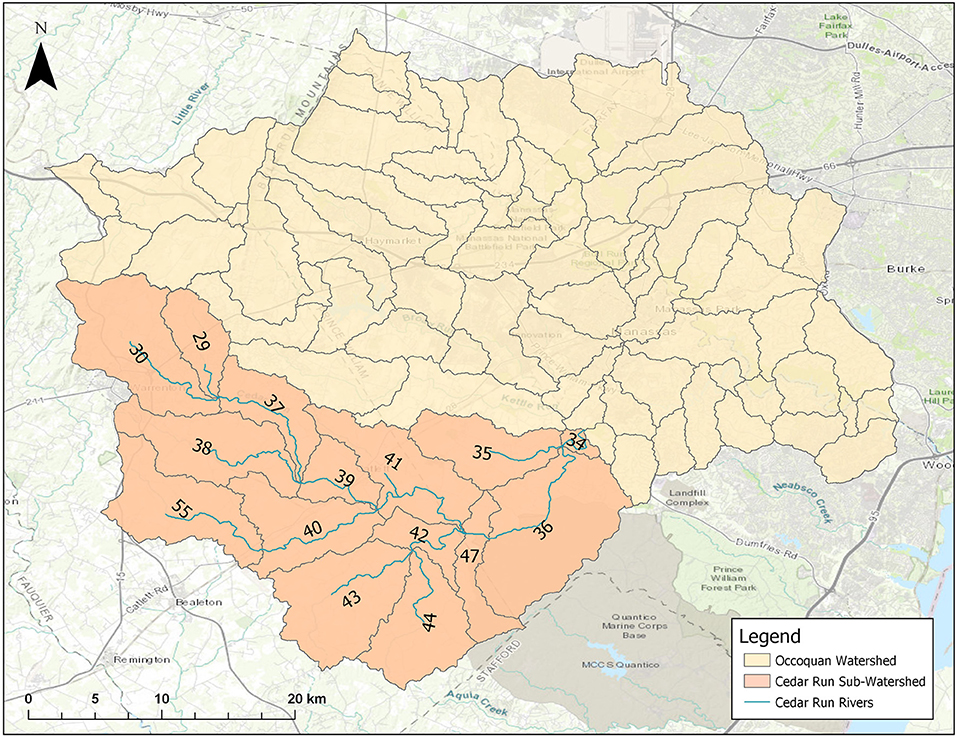
Figure 1. Occoquan Watershed divided into segments with numbered segments representing Cedar Run Sub-watershed.
Fauquier County has a long tradition of agricultural land use. During the 20th century, dairy and beef cattle industry was very prominent within the county. However, this industry has declined within the past several decades. In 1997, 50% of the farms in Fauquier County were devoted to the cattle industry and, by 2012, only 35% of the farms were devoted to this industry. Meanwhile, county grain production remained stable or has slightly increased between 1990 and 2012. Traditional farming has also declined as the number of full-time farmers has decreased by 24% between 2002 and 2012 while the number of part-time farmers has increased by 14% during that same period. In the face of growing human development in the urban areas of the county, officials have specified that they would like to maintain the “rural character” of much of the county by preserving its farmland and ensuring that the county maintains the agricultural sector of its economy. The officials also seek to avoid sprawling urban development and sustain compact settlement patterns. As depicted in Figure 2, these concerns have been addressed through the implementation of zoning districts to restrict land use with about 90% of the county set aside for agriculture (Rephann, 2015; Fauquier County Board of Supervisors, 2019).
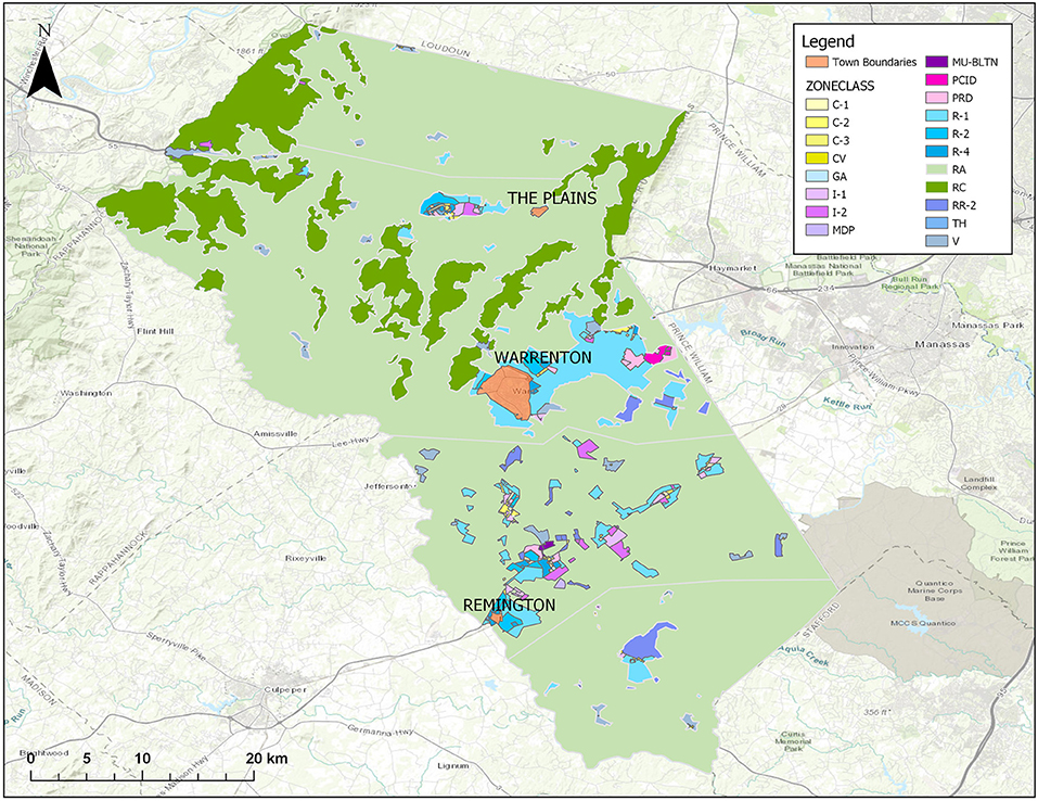
Figure 2. Fauquier County development zones. C1, commercial neighborhood; C2, commercial highway; C3, shopping center; CV, commercial village; GA, garden apartments; I1, industrial park; I2, industrial general; MDP, manufactured dwelling park; MU-BLTN, mixed use Bealeton; PCID, planned commercial industrial development; PRD, planned residential development; R1, residential 1 dwelling unit/acre; R2, residential 2 dwelling unit/acre; R4, residential 4 dwelling unit/acre; RA, rural agriculture; RC, rural conservation; RR2, rural residential; TH, townhouses; V, village.
The most basic I-O model is composed of two model components: the primal quantity model and a price dual model. The primal model calculates economic output for n distinct economic sectors, such as agriculture, manufacturing, and construction, and k factors of production in physical or monetary units of output. Factors of production are required inputs that are themselves not produced, including capital and labor as well as water, land, and other natural resources. The following equations are utilized in the primal model:
where,
A = coefficient matrix (n × n), F = matrix requirements per unit of output (k × n), y = final demand vector (n × 1), x = economic output vector (n × 1), I = identity matrix (n × n), ϕ = factor use vector (k × 1)
The dual model calculates unit cost associated with each economic sector using the following equation:
where,
π = vector of factor prices (k × 1), p = sectoral price vector (n × 1), A′ = transpose of matrix A, F′ = transpose of matrix F.
As an extension of the basic I-O model, RCOT captures interdependencies between consumption and production as well as among sectors dependent on each other's outputs. Additionally, RCOT considers choices among operational technologies based on certain factor constraints. There is a direct interdependence between quantity and cost since a change in availability of a resource or in its unit price can change the choice selection among specific technologies available to different economic sectors (Duchin and Levine, 2011).
RCOT is written as a linear program with n sectors, t technologies, and k factors of production. The primal model specifies t technologies for the n sectors where t ≥ n, which is why the model is referred to as “rectangular.” Parameters and variables distinguish not only among sectors, but also alternative technologies, which are denoted by an asterisk. The primal model utilizes the following objective function:
where,
x* = economic output vector (t × 1), y = final demand vector (n × 1), A* = coefficient matrix (n × t), f = factor endowments vector (k × 1), F* = matrix requirements per unit of output (k × t), π = vector of factor prices (k × 1)
This objective function minimizes factor use while ensuring that production still satisfies final demand (y) and that factor use does not exceed factor availability (f).
The price dual model maximizes the value of final demand net of rents on scarce resources using the following objective function:
where,
y = final demand vector (n × 1), A* = coefficient matrix (n × t), I* = identity matrix (n × t), f = factor endowments vector (k × 1), F* = matrix requirements per unit of output (k × t), p = sectoral prices vector (n × 1), r = factor scarcity rents vector (k × 1)
The endogenous variables in Equation 5 are prices of goods and services (p) and rents on factors that are fully utilized (r). This constraint requires that prices not exceed the cost of production. Therefore, there would be no feasible solution for a specified scenario if the required resource endowments are insufficient to meet the specified consumer demand (Duchin and Levine, 2011).
As mentioned previously, an HSPF model has already been calibrated using local data to represent the hydrological behavior of the Cedar Run Watershed during the 2012 base year. Calibration was carried out using data collected from 2008 to 2010, while the validation process utilized data from 2011 to 2012. This data included regional cloud cover, wind speed, air temperature, and dew point temperature, which were all provided by Washington Dulles International Airport weather station as well as precipitation, which was provided by the rain gauge station located within the watershed. Potential evapotranspiration and solar radiation data were also obtained for calibration using established estimation methods (Xu, 2005; Bartlett, 2013). While there are other more mechanistic models than HSPF as well as more statistical types of watershed models, this model was selected primarily for convenience and because of the long history of successful application in this watershed. Furthermore, it was considered adequate for an initial demonstration of the proposed coupled framework.
HSPF is a structural model designed to represent both natural and developed watersheds. It has the capacity to model both surface and subsurface water quantity and quality. Since it operates in a time series, HSPF represents the processes that are occurring within a specified length of time by generating information at a designated time step that can range from minutes to days. To analyze watershed behavior, HSPF divides the watershed into land and channel segments and the user can utilize the SCHEMATIC block to specify the area and types of land present within these segments. Furthermore, HSPF is composed of application modules used to represent characteristics of each type of segment. One application module, referred to as PERLND, represents permeable land segments, while another module represents impermeable land segments, and a third module is used to represent channel segments. Each of these modules contain sub-modules that simulate specific functions within the segments and these sub-modules can be active or inactive depending on user specifications. In addition to application modules, HSPF also has utility modules that link the application modules and manage the generated data and results (Bicknell et al., 2001).
Water quantity processes that are modeled within the PERLND module are primarily controlled by the sub-module PWATER. The purpose of this sub-module is to simulate the water budget for each pervious land segment, which is accomplished using a water budget equation to predict total runoff from a pervious surface. Additionally, the PQUAL sub-module is used to simulate the movement and fate of water quality constituents from pervious surfaces to the outflows, such as nitrate, phosphorus, and sediments produced by land erosion. On impervious surfaces, the water budget is determined by a sub-module that determines how much moisture is retained within the land segment and how much of that moisture becomes runoff or evaporates. Furthermore, another sub-module simulates the hydraulic behavior of the water within each channel segment and functions under the assumption that complete mixing and unidirectional flow occurs within each channel segment. To determine the appropriate function for outflow from the channel, the user must specify the fate of the outflow, such as whether it will flow into an open channel or if it will be withdrawn for irrigation or other purposes (Bicknell et al., 2001).
In this application of a coupled modular framework (Figure 3), changes within the watershed are driven by the optimized economic model. Changes in economic activity within a watershed are represented by changing the final demand associated with the specified sectors within the economy. These values are exogenous variables presented in the y vector of RCOT and can reflect real-world changes, such as an expansion of residents or an increase in production of goods and services. Furthermore, the exogenous variables presented in the f vector of RCOT, factor endowments, would include not only the workforce and capital available for economic activity, but also the land and water available within the watershed.
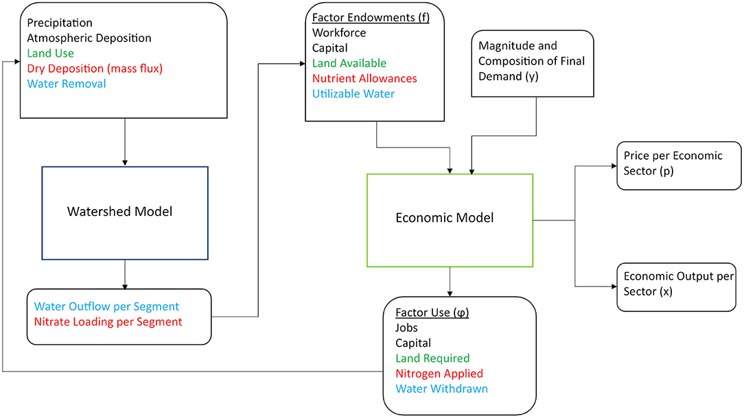
Figure 3. Conceptual modular framework for coupling a constrained optimization economic model (RCOT) with a watershed model (HSPF). Green- units of land use, Red- units of nitrogen, Blue- units of water, Sharp-edged rectangles- modeling software, Soft/Sharp-edged rectangles- model inputs, Soft-edged rectangles- model outputs.
Once these variables are input into RCOT, the economic model is run to obtain endogenous variables. These variables include the economic output from each sector, presented in the x vector of the model, and the factor quantities required to achieve final demand, which are presented in the ϕ vector. Price per economic sector would also be output in the p vector produced by the dual price model of RCOT. These vectors are shown in Figure 3 as outputs from the economic model.
Several values of output from the ϕ vector of RCOT's primal model can be used to couple the economic model with the watershed model, specifically the land required, water withdrawn, and the fertilizer applied to achieve final demand. The input characteristics of the HSPF watershed model are adjusted to reflect these changes in factor use. Since RCOT presents these output values in physical units, the transfer of information to HSPF is straightforward. Each watershed segment is divided into different land use categories, which are each defined based on land surface permeability. Increases in land requirements from RCOT translate into changes in area associated with these different categories of land and are exogenously defined within the SCHEMATIC block of HSPF. Additionally, increases in water withdrawals translate into exogenous changes in point source water extraction from the watershed within the PWATER sub-module of HSPF and increases in nitrogen application translate into exogenous changes in the dry deposition of nutrients, such as nitrate, ammonia, or a combination of the two, within the watershed using the PQUAL sub-module.
Once the characteristics of the watershed have been adjusted in response to the changes in economic activity, HSPF is run to determine the fate of the water and applied nutrients, resulting in the endogenous variables of water quantity and nutrient concentrations that flow through each segment of the watershed. These outputs, shown in Figure 3, are dependent on parameters, such as precipitation, runoff, and infiltrations rates, that have been previously established during the HSPF model calibration process. Finally, the water availability and nutrient allowances presented in the f vector must be adjusted to reflect the physical changes that have occurred within the watershed because of previous economic activity before RCOT may be run for the next timestep. If more water is withdrawn from the watershed to support current economic expansion, then less water will be available for any future economic expansion. As a result, a more water-efficient management practice may be implemented in different sectors, even if it is more expensive than the standard practice because one of RCOT's objective functions is to minimize factor use. Thus, this framework captures how changes in economic activity will alter the physical conditions within a watershed and how these physical changes will in turn limit economic activity or influence economic decisions.
This study requires the construction of a county-level database to represent Fauquier County's economy and to distinguish between the sectors of interest for this analysis. Fortunately, monetary county-level, input-output data is available from a private company called IMPLAN Group LLC (2016). IMPLAN Group compiles their county-level datasets by gathering data from various sources, including the United States Bureau of Economic Analysis (BEA) and Bureau of Labor Statistics (BLS), and providing estimates for unavailable data while benchmarking them against other data to ensure as much accuracy as possible. Economic data was obtained for Fauquier County representative of the year 2012, which serves as the base year. To begin, the county input-output transaction table (Z) and industry final demand data (y) provided by IMPLAN Group were aggregated into seven basic industrial sectors using an aggregation matrix and following the guidelines provided by Miller and Blair (2009). These sectors, including agriculture, mining, construction, manufacturing, utilities, professional services, and government services, were aggregated based on the North American Industry Classification System (NAICS) established by the United States Census Bureau (2017). Once the transaction table was aggregated, the technical coefficient (A) matrix was calculated using the data from the transaction table and economic output data provided by IMPLAN Group, as follows:
Next, the agriculture sector was disaggregated into three specific sectors, crop farming, animal husbandry, and other agricultural activities, for a more detailed analysis. The finalized A matrix is displayed in Table 1. Total sector output was calculated for the 2012 base year using this A matrix as well as the aggregated final demand (y) vector (Equation 1). The resulting output (x) vector was compared to the sector output data provided by IMPLAN Group for 2012 in order to verify that this model accurately represents the economy of Fauquier County. The results produced by the model were within the same range as the provided data.
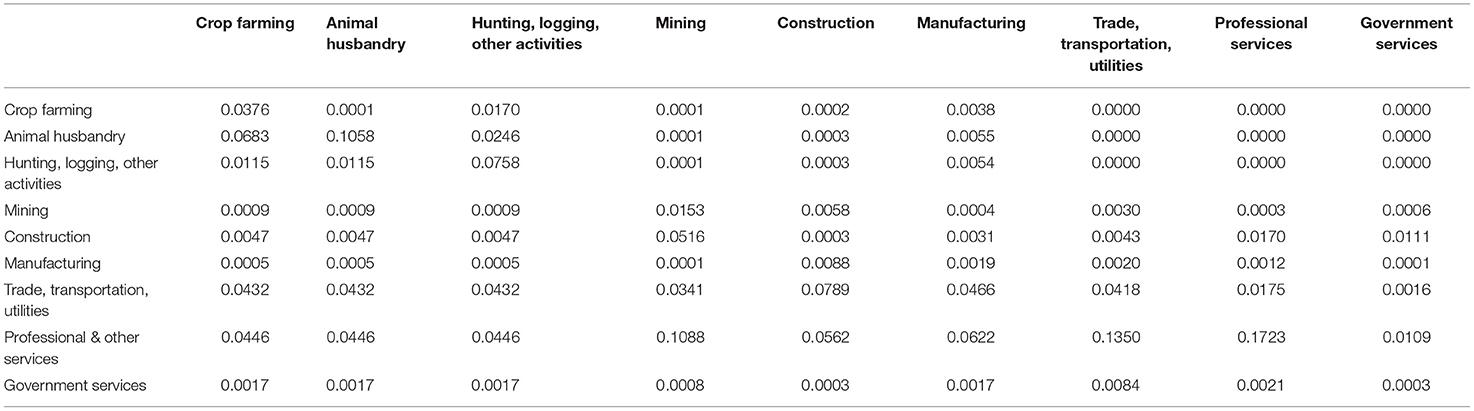
Table 1. Technical coefficient matrix (A) for Fauquier County 2012.
To build the factor requirement per unit of output (F) matrix, six factors of production were identified as requirements for each sector, specifically land, labor, capital, water withdrawn, nitrogen applied as fertilizer and nitrogen applied as manure. Annual labor and capital requirements were calculated using IMPLAN sectoral data for labor, capital, and economic output. Water withdrawn per unit of output for each sector was determined using county water data available from the United States Geological Survey (USGS, 2010) as well as data obtained from an input-output database assembled by the Green Design Institute at Carnegie Mellon University (Blackhurst et al., 2010). Additionally, fertilizer requirements were assumed based on county data available from the National Agricultural Statistics Service (NASS). Furthermore, land requirements per sector were assumed based on county zoning data provided by the Fauquier County GIS Office (2014). However, these land requirements had to be adjusted since the zoning data did not consider land that had not been developed or cleared for a specific use. Therefore, land cover data obtained from the Virginia Geographic Information Network (VGIN, 2016) was used in combination with the zoning data to determine how much land in each zone was cleared or wooded, which was assumed to be an indicator of developed and undeveloped land, respectively.
The economic database was established using Fauquier County data from 2012 and an HSPF model had already been calibrated and validated to represent Cedar Run Watershed using local data collected between 2008 and 2012. This data was then used to analyze a set of illustrative scenarios intended to demonstrate the power of the modeling approach and the capabilities of the coupled framework. These scenarios were performed at the annual time scale. All inputs and outputs for the economic model are representative of 1 year of economic activity. The annual nitrogen requirement was then disaggregated to the monthly scale so that it could be utilized in the watershed model. It was assumed that each month received 1/12 of the nitrogen applied as manure while the month of March received all the nitrogen applied as fertilizer for croplands and the month of August received all the nitrogen applied as fertilizer for pasture to simply represent seasonal applications of fertilizer. Then, the outflow results produced by HSPF were aggregated from the daily to the annual scale to determine the average annual nitrogen loading.
These scenarios are dramatizations that were developed based on assumptions about human activities within the watershed and using attributes of the Fauquier County database but could be generalized to represent other locations with more complex water quantity and quality issues. In this case, expansions in agricultural industries, specifically crop farming or animal husbandry, were examined because more agricultural land use could be considered more acceptable by the County since it would discourage urban development and maintain the desired rural aesthetic. Since this framework was modeling static conditions within the 1-year simulation period, the agricultural expansion was assumed to have occurred sometime before rather than during the simulation period. Furthermore, since these scenarios were not being used to predict conditions during a specific future year, the time value of money was not considered, and it was assumed that monetary valuation remained constant across all scenarios. Thus, money values are in constant base-year prices. Additionally, since water scarcity was not considered to be a major issue in the county, it was not explored in this study. It was also assumed that the population of the county residents does not significantly increase so there is insignificant urban development. In-migrants are assumed to work in the same sectors as the current labor force and increase output only from existing economic sectors. Furthermore, in-migrants who are retired, work outside the county, or are just seasonal residents were not considered.
For the baseline scenarios (referred to as S1 and S2 in Table 2), the basic I-O model was used to determine how a dramatic increase in production from an agricultural sector, represented by an increase in final demand in the y vector, would result in an increase in economic output from that sector, but would also require an increase in use of factors of production, specifically land, labor, water, and applied nitrogen. Thus, the basic I-O model was used to determine how expanding final demand by an amount necessary to fully utilize all land available for agriculture would impact water quality, represented by the concentration of nitrogen outflow from the local watershed. In S1, demand for crop farming was expanded to achieve a 270% increase in land used for crop farming. In S2, demand for animal husbandry was expanded to achieve a 220% increase in land used for animal husbandry. In these two scenarios, it was assumed that the increase in land use associated with the expansion of agricultural activity is equally distributed among the HSPF land segments and that land classified as forest in HSPF is converted to cropland in S1 and pasture in S2. Furthermore, the increase in applied nitrogen associated with the expansion of agricultural activity was assumed to increase nitrate deposition in HSPF during the month of March for cropland and during August for pasture, to correspond with fertilizer application.
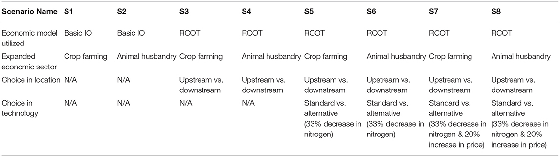
Table 2. Summary of scenarios.
In S3, S5, and S7, demand for crop farming was increased to achieve a 270% increase in land use as was done in S1. In S4, S6, and S8, demand for animal husbandry was increased to achieve a 220% increase in land use as was done in S2. The differences among these scenarios are summarized in Table 2. Unlike S1 and S2, S3 through S8 utilize RCOT instead of the basic I-O model to evaluate alternatives for alleviating the rising nitrate concentrations that result from the dramatic increase in production from either crop farming or animal husbandry. In these scenarios, the choice mechanism of RCOT was used to select between two locations to obtain an optimal distribution of agricultural activity. For RCOT, the watershed is comprised of two super-segments, Upstream and Downstream, each comprised of multiple HSPF segments and RCOT specifies how much activity will take place in each individual segment of the two sets of segments shown in Figure 4. Thus, the expansion in agricultural activity is no longer assumed to be equally distributed as it was in S1 and S2. Furthermore, these scenarios assume that different factor endowments are available in each location. More land was assumed to be available in Upstream for expansion of agricultural activities than in Downstream. Residential and industrial land use is predominantly located in Upstream along with water withdrawn for domestic use, which results in higher excess nutrient concentration in Upstream than in Downstream. As a result, it is assumed that less water is available and less nutrient runoff is allowable from agricultural expansion in Upstream rather than in Downstream.
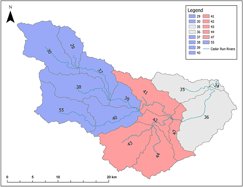
Figure 4. Cedar Run Watershed with Upstream (blue) defined as segments 29, 30, 37, 38, 39, 40, 55 and Downstream (red) defined as segments 41, 42, 43, 44, 47.
In S5 through S8, a choice in practice was incorporated into RCOT in addition to the choice in production location. In S5 and S6, a hypothetical alternative management practice was introduced that reduced fertilizer requirements for crop farming and animal husbandry by 33%. In S7 and S8, a hypothetical alternative management practice was also introduced into RCOT that could reduce fertilizer requirements by 33% but would also cost 20% more than the standard practice. Thus, RCOT was used in these scenarios to select between two locations to obtain an optimal distribution of agricultural activity and to choose between two management practices to minimize factor use and to maximize the value of final demand.
Table 3 presents the economic modeling results for each scenario, specifically from the ϕ and x vectors. These outputs are listed as percent increases relative to the outputs obtained from 2012, the economic base year. When crop farming was expanded in S1, S3, S5, and S7, the acres of cropland increased by 270% regardless of the configuration of the economic model. Additionally, these scenarios also produced similar increases in jobs (~7.8%), water withdrawn (~5.7%), and economic output (~1.8%) within the county. Furthermore, these scenarios also resulted in a 240% increase in applied nitrogen except for S5, which only resulted in a 130% increase in applied nitrogen. When animal husbandry was expanded in S2, S4, S6, and S8, the acres of pasture increased by 220% regardless of the configuration of the economic model. These scenarios also produced similar increases in jobs (~2.6%), water withdrawn (~3.4%), and economic output (~0.9%) within the county. Additionally, these scenarios resulted in a 23% increase in applied nitrogen except for S6, which only resulted in a 17% increase in applied nitrogen.
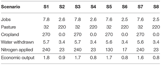
Table 3. Percent increases in ϕ and x vector outputs relative to 2012 base year.
When the output results for land use and applied nitrogen (Table 3) were transferred from the economic model to HSPF, the total nitrogen concentration of watershed outflow from Cedar Run Watershed was obtained based on HSPF output results aggregated to the annual scale. Table 4 presents the nitrogen concentrations achieved by each scenario. When crop farming was expanded in S1, nitrogen concentration in the watershed outflow increased from 0.6 to 4.3 mg/L and when animal husbandry was expanded in S2, nitrogen concentration increased from 0.6 to 0.7 mg/L. When RCOT was only used to determine optimal distribution of agricultural activity, nitrogen concentration increased from 0.6 to 4.2 mg/L for S3, and from 0.6 to 0.7 mg/L for S4. When RCOT was used to select optimal management practice in addition to spatial distribution of agricultural activity, nitrogen concentration increased from 0.6 to 2.6 mg/L for S5 and from 0.6 to 0.7 mg/L for S6. When a higher cost was associated with the alternative practice, nitrogen concentration increased from 0.6 to 4.2 mg/L for S7 and from 0.6 to 0.7 mg/L for S8.
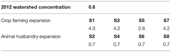
Table 4. Concentration of total nitrogen in watershed outflow (mg/L).
An increase in economic demand caused by an expansion of crop farming resulted in an increase in jobs that is about three times larger than what resulted from an expansion of animal husbandry. Additionally, the crop farming expansion resulted in a 1.8% increase in economic output, which is about double the increase in economic output that resulted from the expansion in animal husbandry (0.9%). These results were achieved regardless of whether the basic I-O or RCOT model was used. Therefore, an expansion in crop farming would be more desirable than an expansion in animal husbandry when examining these scenarios from an economic perspective.
In addition to higher increases in jobs and economic output, a crop farming expansion also resulted in a slightly higher increase in annual water withdrawal than an animal husbandry expansion, but both increases in water withdrawal were considered insignificant when compared to the quantity of water available within Cedar Run Watershed. However, the crop farming expansion also resulted in a significantly higher increase in fertilizer applied annually within the watershed than the animal husbandry expansion. As a result, the crop farming expansion increased the concentration of nitrogen in Cedar Run Watershed by 3.7 mg/L in S1 while the animal husbandry expansion had insignificant effects on nitrogen concentration in S2. Thus, while a crop farming expansion results in a higher increase in jobs and economic output, it also results in a significantly higher application of nitrogen and a significantly higher impact on the nitrogen outflow concentration than an animal husbandry expansion. Therefore, an expansion of animal husbandry would be more acceptable than a crop farming expansion when analyzing these results from an environmental perspective.
The results from S1 and S2 demonstrate the trade-offs associated with expansions in crop farming or animal husbandry. The results from S3 through S8 indicate how choices made within the economic system could alleviate the severity of the nitrate loading. When the choice between Upstream and Downstream was implemented using RCOT, the resulting nitrogen concentration in S3 was insignificantly lower than in S1. However, when choice in management practice was implemented in S5, the resulting nitrogen concentration from crop farming expansion reached only 2.6 mg/L at the outflow of Cedar Run Watershed, which is about 50% lower than in S1 when only the standard technology could be applied. Therefore, alternative technologies appear to be more effective at alleviating water quality issues than optimal spatial distribution of economic activity. However, when the cost associated with the alternative practice was increased to 120% of the standard practice cost in S7, RCOT selected the standard practice over the alternative practice. As a result, the corresponding nitrogen concentration was as high as it was in S3. Thus, when a more efficient practice was introduced as an alternative during expansions in either crop farming or animal husbandry, this practice was selected by RCOT because it required less fertilizer, which resulted in a lower increase in nitrogen concentration from expanded crop farming. Nevertheless, when the alternative practice was introduced with a higher price, RCOT selected the standard practice because it was the more cost-effective option. Interestingly, the introduction of alternative choices had little impact on the increase in nitrogen concentration that resulted from animal husbandry expansion because this economic sector already utilizes significantly less fertilizer than the crop farming sector. The nitrogen concentration resulting from animal husbandry expansion remained at around 0.7 mg/L, regardless of the choices considered by RCOT. Therefore, implementing the alternative practice within the animal husbandry sector may be unnecessary in terms of alleviating impacts on water quality.
A framework that couples economic and watershed systems can capture the interactions between these two systems and can also be used to analyze how changes in economic activity will impact watershed health. However, selecting the appropriate economic model requires careful consideration and more detailed information could be obtained depending on which model is utilized. When the basic I-O model was coupled with HSPF, we were able to capture the changes in water quality associated with an expansion in economic activity. However, when RCOT was coupled with HSPF, more detailed information could be obtained about how choices in spatial location or technology could influence economic activity and alter impacts on watershed health. These are realistic decisions that may be made within the economic system and, by linking RCOT with HSPF, the environmental impacts of these choices can be examined.
Building on the modular framework, future work will involve designing more complex scenarios that can test policy options and regional planning decisions. The simple example presented in this paper focused primarily on the influence of the economic system on the natural system, but in the future, scenarios will be developed that look more closely at how the natural system affects the economic system and that will couple the models more intimately. Additionally, this modular framework should also be applied in a more complex location with a greater number of economic sectors of interest and pressing environmental concerns. The multi-region capabilities of RCOT could also be explored in a region located within a watershed that spans multiple economic systems. The modular framework is also appropriate for a system-of-systems approach that integrates a variety of models from different disciplines and modeling paradigms to represent a socio-environmental (or social-ecological) system, and that can be used to inform policy and decision-making processes (Little et al., 2016, 2019; Iwanaga et al., 2021).
MA and JL conceived of the presented idea. MA designed the conceptual modeling framework and built the economic database. MA and AB modified the HSPF code and its output configuration. CL-M provided RCOT code using Lingo software and advised on the configuration of the RCOT matrices. JL supervised the project. MA drafted the manuscript and designed the figures with the support of AB, CL-M, and JL, who all provided comments and suggestions. All authors contributed to the article and approved the submitted version.
We acknowledge funding from the National Science Foundation (NSF) Award EEC-1937012 as well as workshop support from the National Socio-Environmental Synthesis Center (SESYNC) under funding received from NSF DBI-1639145.
AB was employed by the company Artasol, LLC.
The remaining authors declare that the research was conducted in the absence of any commercial or financial relationships that could be construed as a potential conflict of interest.
We would like to express our deep appreciation to Dr. Faye Duchin for her substantial and valuable input and for her willingness to engage so generously during this research.
Bartlett, J. A. (2013). Heuristic Optimization of Water Reclamation Facility Nitrate Loads for Enhanced Reservoir Water Quality (Doctor of Philosophy). Virginia Polytechnic Institute and State University.
Bicknell, B. R., Imhoff, J. C., Kittle, J. L, Jobes, T. H., and Donigian, A. S. (2001). Hydrological Simulation Program-FORTRAN. User's Manual for Release 12. US EPA.
Blackhurst, M., Hendrickson, C., and Vidal, J. S. (2010). Direct and indirect water withdrawals for U.S. industrial sectors. Environ. Sci. Technol. 44, 2126–2130. doi: 10.1021/es903147k
Bohringer, C., and Loschel, A. (2006). Computable general equilibrium models for sustainability impact assessment: status quo and prospects. Ecol. Econ. 60, 49–64. doi: 10.1016/j.ecolecon.2006.03.006
Brouwer, R., and Hofkes, M. (2008). Integrated hydro-economic modelling: approaches, key issues and future research directions. Ecol. Econ. 66, 16–22. doi: 10.1016/j.ecolecon.2008.02.009
Cai, X., McKinney, D. C., and Lasdon, L. S. (2003). Integrated hydrologic-agronomic-economic model for river basin management. J. Water Resour. Plann. Manage. 129, 4–17. doi: 10.1061/(ASCE)0733-9496(2003)129:1(4)
Cai, X. M., Ringler, C., and You, J. Y. (2008). Substitution between water and other agricultural inputs: implications for water conservation in a River Basin context. Ecol. Econ. 66, 38–50. doi: 10.1016/j.ecolecon.2008.02.010
Duchin, F. (2005). A world trade model based on comparative advantage with m regions, n goods, and k factors. Econ. Syst. Res. 17, 141–162. doi: 10.1080/09535310500114903
Duchin, F., and Levine, S. H. (2011). Sectors may use multiple technologies simultaneously: the rectangular choice-of-technology model with binding factor constraints. Econ. Syst. Res. 23, 281–302. doi: 10.1080/09535314.2011.571238
Duchin, F., and Levine, S. H. (2012). The rectangular sector-by-technology model: not every economy produces every product and some products may rely on several technologies simultaneously. J. Econ. Struct. 1:1e11. doi: 10.1186/2193-2409-1-3
Escriva-Bou, A., Pulido-Velazquez, M., and Pulido-Velazquez, D. (2017). Economic value of climate change adaptation strategies for water management in Spain's Jucar Basin. J. Water Resour. Plann. Manag. 143:04017005. doi: 10.1061/(ASCE)WR.1943-5452.0000735
Esteve, P., Varela-Ortega, C., Blanco-Gutierrez, I., and Downing, T. E. (2015). A hydro-economic model for the assessment of climate change impacts and adaptation in irrigated agriculture. Ecol. Econ. 120, 49–58. doi: 10.1016/j.ecolecon.2015.09.017
Fauquier County Board of Supervisors (2019). Chapter 8: Rural Land Use Plan. Retrieved from: https://www.fauquiercounty.gov/home/showdocument?id=7216 (accessed May 10, 2021).
Fauquier County GIS Office (2014). Fauquier County Zoning GIS Data [GIS Shape Files]. Warrenton, VA. Available from: https://www.fauquiercounty.gov/government/departments-a-g/gis-mapping/gis-data (accessed May 10, 2021).
Harou, J. J., Pulido-Velazquez, M., Rosenberg, D. E., Medellin-Azuara, J., Lund, J. R., and Howitt, R. E. (2009). Hydro-economic models: concepts, design, applications, and future prospects. J. Hydrol. 375, 627–643. doi: 10.1016/j.jhydrol.2009.06.037
IMPLAN Group LLC (2016). IMPLAN 2011-2013 Fauquier County Data [Data sets and Excel Sheets]. Huntersville, NC. Available from: https://implan.com (accessed May 10, 2021).
Iwanaga, T., Wang, H.-H., Hamilton, S. H., Grimm, V., Koralewski, T. E., Salado, A., et al. (2021). Socio-technical scales in socio-environmental modeling: managing a system-of-systems modeling approach. Environ. Model. Softw. 135:104885. doi: 10.1016/j.envsoft.2020.104885
Jiang, L., Wu, F., Liu, Y., and Deng, X. Z. (2014). Modeling the impacts of urbanization and industrial transformation on water resources in China: an integrated hydro-economic CGE analysis. Sustainability 6, 7586–7600. doi: 10.3390/su6117586
Jonkman, S. N., Bockarjova, M., Kok, M., and Bernardini, P. (2008). Integrated hydrodynamic and economic modelling of flood damage in the Netherlands. Ecol. Econ. 66, 77–90. doi: 10.1016/j.ecolecon.2007.12.022
Kahil, M. T., Ward, F. A., Albiac, J., Eggleston, J., and Sanz, D. (2016). Hydro-economic modeling with aquifer-river interactions to guide sustainable basin management. J. Hydrol. 539, 510–524. doi: 10.1016/j.jhydrol.2016.05.057
Kahsay, T. N., Arjoon, D., Kuik, O., Brouwer, R., Tilmant, A., and van der Zaag, P. (2019). A hybrid partial and general equilibrium modeling approach to assess the hydro-economic impacts of large dams - The case of the Grand Ethiopian Renaissance Dam in the Eastern Nile River basin. Environ. Econ. 117, 76–88. doi: 10.1016/j.envsoft.2019.03.007
Kelly, R. A., Jakeman, A. J., Barreteau, O., Borsuk, M. E., ElSawah, S., Hamilton, S. H., et al. (2013). Selecting among five common modelling approaches for integrated environmental assessment and management. Environ. Model. Softw. 47, 159–181. doi: 10.1016/j.envsoft.2013.05.005
Knowling, M. J., White, J. T., McDonald, G. W., Kim, J. H., Moore, C. R., and Hemmings, B. (2020). Disentangling environmental and economic contributions to hydro-economic model output uncertainty: an example in the context of land-use change impact assessment. Environ. Model. Softw. 127:104653. doi: 10.1016/j.envsoft.2020.104653
Little, J. C., Hester, E. T., and Carey, C. C. (2016). Assessing and enhancing environmental sustainability: a conceptual review. Environ. Sci. Technol. 50, 6830–6845. doi: 10.1021/acs.est.6b00298
Little, J. C., Hester, E. T., Elsawah, S., Filz, G. M., Sandu, A., Carey, C. C., et al. (2019). A tiered, system-of-systems modeling framework for resolving complex socio-environmental policy issues. Environ. Model. Softw. 112, 82–94. doi: 10.1016/j.envsoft.2018.11.011
Lopez-Morales, C., and Duchin, F. (2015). Economic implications of policy restrictions on water withdrawals from surface and underground sources. Econ. Syst. Res. 27, 154–171. doi: 10.1080/09535314.2014.980224
Lopez-Morales, C., and Rodriguez-Tapia, L. (2019). On the economic analysis of wastewater treatment and reuse for designing strategies for water sustainability: lessons from the Mexico Valley Basin. Resour. Conserv. Recycl. 140, 1–12. doi: 10.1016/j.resconrec.2018.09.001
Lund, J. R., Cai, X. M., and Characklis, G. W. (2006). Economic engineering of environmental and water resource systems. J. Water Resour. Plann. Manag. 132, 399–402. doi: 10.1061/(ASCE)0733-9496(2006)132:6(399)
McKitrick, R. R. (1998). The econometric critique of computable general equilibrium modeling: the role of functional forms. Econ. Model. 15, 543–573. doi: 10.1016/S0264-9993(98)00028-5
Miller, R. E., and Blair, P. D. (2009). Input-Output Analysis: Foundations and Extensions, 2nd Edn. Cambridge University Press.
Pulido-Velazquez, M., Andreu, J., Sahuquillo, A., and Pulido-Velazquez, D. (2008). Hydro-economic river basin modelling: the application of a holistic surface-groundwater model to assess opportunity costs of water use in Spain. Ecol. Econ. 66, 51–65. doi: 10.1016/j.ecolecon.2007.12.016
Rephann, T. J. (2015). Fauquier County Cost of Community Services Study. Weldon Cooper Center for Public Service, University of Virginia.
Scrieciu, S. S. (2007). The inherent dangers of using computable general equilibrium models as a single integrated modelling framework for sustainability impact assessment. A critical note on Bohringer and Loschel (2006). Ecol. Econ. 60, 678-684. doi: 10.1016/j.ecolecon.2006.09.012
United States Census Bureau (2017). North American Industry Classification System. Retrieved from: https://www.census.gov/naics/ (accessed May 10, 2021).
USGS (2010). Estimated Use of Water in the United States County-Level Data for 2010 [Excel Format]. United States Geological Survey. Retrieved from: https://water.usgs.gov/watuse/data/2010/index.html (accessed May 10, 2021).
VGIN (2016). Land Cover Dataset: Bay Area 2 [GIS Shape Files]. Virginia Geographic Information Network. Retrieved from: https://ftp.vgingis.com/download_2/land_cover/Bay_Area_2/ (accessed May 10, 2021).
Xu, Z. (2005). A Complex, Linked Watershed-Reservoir Hydrology and Water Quality Model Application for the Occoquan Watershed, Virginia (Doctor of Philosophy). Virginia Polytechnic Institute and State University.
Xu, Z., Godrej, A, N., and Grizzard, T. J. (2007). The hydrological calibration and validation of a complexly linked watershed-reservoir model for the Occoquan watershed, Virginia. J. Hydrol. 345, 167–183. doi: 10.1016/j.jhydrol.2007.07.015
Zhang, X. G. (2013). “A simple structure for CGE models,” in Paper presented at the 16th Annual Conference on Global Economic Analysis, Shanghai, China. Retrieved from: https://www.gtap.agecon.purdue.edu/resources/res_display.asp?RecordID=4157 (accessed May 10, 2021).
Keywords: modeling, framework, economic, hydrologic, watershed
Citation: Amaya M, Baran A, Lopez-Morales C and Little JC (2021) A Coupled Hydrologic-Economic Modeling Framework for Scenario Analysis. Front. Water 3:681553. doi: 10.3389/frwa.2021.681553
Received: 16 March 2021; Accepted: 29 April 2021;
Published: 03 June 2021.
Edited by:
Amin Elshorbagy, University of Saskatchewan, CanadaReviewed by:
Ahmed Abdelkader, University of Saskatchewan, CanadaCopyright © 2021 Amaya, Baran, Lopez-Morales and Little. This is an open-access article distributed under the terms of the Creative Commons Attribution License (CC BY). The use, distribution or reproduction in other forums is permitted, provided the original author(s) and the copyright owner(s) are credited and that the original publication in this journal is cited, in accordance with accepted academic practice. No use, distribution or reproduction is permitted which does not comply with these terms.
*Correspondence: John C. Little, amNsQHZ0LmVkdQ==
Disclaimer: All claims expressed in this article are solely those of the authors and do not necessarily represent those of their affiliated organizations, or those of the publisher, the editors and the reviewers. Any product that may be evaluated in this article or claim that may be made by its manufacturer is not guaranteed or endorsed by the publisher.
Research integrity at Frontiers
Learn more about the work of our research integrity team to safeguard the quality of each article we publish.