 Ahmad Momeni
 Kalyan R. Piratla
- Glenn Department of Civil Engineering, Clemson University, Clemson, SC, United States
It is estimated that about 20% of treated drinking water is lost through distribution pipeline leakages in the United States. Pipeline leakage detection is a top priority for water utilities across the globe as leaks increase operational energy consumption and could also develop into potentially catastrophic water main breaks, if left unaddressed. Leakage detection is a laborious task often limited by the financial and human resources that utilities can afford. Many conventional leak detection techniques also only offer a snapshot indication of leakage presence. Furthermore, the reliability of many leakage detection techniques on plastic pipelines that are increasingly preferred for drinking water applications is questionable. As part of a smart water utility framework, this paper proposes and validates a hydraulic model-based technique for detecting and assessing the severity of leakages in buried water pipelines through monitoring of pressure from across the water distribution system (WDS). The envisioned smart water utility framework entails the capabilities to collect water consumption data from a limited number of WDS nodes and pressure data from a limited number of pressure monitoring stations placed across the WDS. A popular benchmark WDS is initially modified by inducing leakages through addition of orifice nodes. The leakage severity is controlled using emitter coefficients of the orifice nodes. WDS pressure data for various sets of demands is subsequently gathered from locations where pressure monitoring stations are to be placed in that modified distribution network. An evolutionary optimization algorithm is subsequently used to predict the emitter coefficients so as to determine the leakage severities based on the hydraulic dependency of the monitored pressure data on various sets of nodal demands. Artificial neural networks (ANNs) are employed to mimic the popular hydraulic solver EPANET 2.2 for high computational efficiency. The goals of this study are to: (1) validate the proof of concept of the proposed modeling approach for detecting and assessing the severity of leakages and (2) evaluate the sensitivity of the prediction accuracy to number of pressure monitoring stations and number of demand nodes at which consumption data is gathered and used. This study offers new value to prioritize pipes for rehabilitation by predicting leakages through a hydraulic model-based approach.
Introduction
As the increasing paucity of water resources and the fast-growing water demands (Gupta and Kulat, 2018) in water distribution systems (WDSs) as a critical infrastructure in societies loom ahead, sustainable maintenance of WDSs operationally and financially is of an utmost essence (Gupta and Kulat, 2018; Momeni et al., 2018; Zhang K. et al., 2019; Al Qahtani et al., 2020; Shukla and Piratla, 2020). Specifically, leakage in WDSs reportedly makes up between 5 and 50 percent of the total freshwater losses depending on the conditions of the pipelines in developed countries (Gupta and Kulat, 2018; Sophocleous et al., 2019; Shukla and Piratla, 2020; Yazdekhasti et al., 2020). It is also estimated that a significant portion of catastrophic pipe breaks stems from undetected and thus unaddressed minor or moderate leaks as well as poor fittings (Grigg, 2017; Gupta and Kulat, 2018; Xie et al., 2019). Besides, detecting and addressing leakages in metallic and plastic pipelines through conventional techniques are found to be disputable, for instance, due respectively to difficulty in localizing welded joint failures (Zhang W. et al., 2018) and inaccuracies of low-frequency detection of plastic materials acting as low-pass filters (Gao et al., 2017). However, conventional leakage detection techniques are per se inclusive of cumbersome tasks which incur massive operational costs and are often labor-intensive (Liu et al., 2019; Ma et al., 2019). Hence, a systematic data-driven background leakage detection offering high accuracy and cost-effectiveness in WDSs plays an integral part in pinpointing and addressing the leak sources to both optimize energy consumption and prevent major future pipe breaks across a network (Gupta and Kulat, 2018; De Marchis and Milici, 2019). Recently, data-driven schemes of detecting and measuring the severity of leaks have been proposed to offer a paradigm shift. For instance, an estimation of life-cycle cost and energy consumption of a sensor-based, network-wide leakage monitoring detection system has been conducted (Yazdekhasti et al., 2020). Also, multiscale neural networks as well as various multi-objective optimization methods have been leveraged to employ consumption data for localization of leaks in a WDS (Creaco and Haidar, 2019; Zhang K. et al., 2019; Shukla and Piratla, 2020; Hu et al., 2021). However, what these methods seem to share is (i) relying partly on either human intervention or expensive tools and (ii) focusing mostly on detecting rather than measuring the severity of leaks with high accuracies. A hydraulic-model-based scheme for leakage detection and most importantly severity assessment could offer promise given the growing adoption of smart water meters and continuous hydraulic monitoring of WDSs. As a result, building upon previous studies (Momeni et al., 2018, 2020; Piratla and Momeni, 2019; Momeni and Piratla, 2021), this paper (i) offers a preliminary proof-of-concept study of a fully data-driven hydraulic model-based prediction paradigm leveraging pressure monitoring data where not only are leak sources detected, but also their severities captured with a reasonable accuracy and (ii) conducts a series of sensitivity analyses of the very prediction model to the number and placement of smart meters and pressure monitoring stations. This preliminary study proves novel by shedding light on a wider scope of how consumption data can be leveraged to minimize the risk of major pipe breaks due to difficult-to-detect leaks without entirely relying on manual inspection techniques and consequently imposing less maintenance costs on municipalities.
Materials and Methods
The fundamental methodology in this paper is to predict the leakage presence and its severity using a reverse-engineering data-driven condition assessment scheme by employing artificial neural networks (ANNs) and genetic algorithms (GA) for a modified version of Hanoi (Fujiwara and Khang, 1990; Piratla and Momeni, 2019) benchmark WDS. Consumption data (nodal demands from smart meters) and pressure monitoring data from the WDS are fed into neural networks in MATLAB 2020a to circumvent the time-consuming EPANET 2.2 hydraulic simulator toolkit. Then, the trained networks will be leveraged in genetic algorithms to predict the induced leakage by mimicking it through emitter nodes.
Hanoi Water Distribution Network Demonstration
Hanoi benchmark WDS, a metallic three-looped network, is modified by including emitter nodes in the middle of pipes to characterize the leakage at each pipe. Since this paper studies leakages at some of the pipes in Hanoi, emitter nodes are randomly placed on six and 12 pipes to establish two cases of actual leakage induction. Figure 1 shows the placement of such emitters for the two cases in Hanoi WDS. Table 1 represents the original Hanoi network geometric and hydraulic specifications.
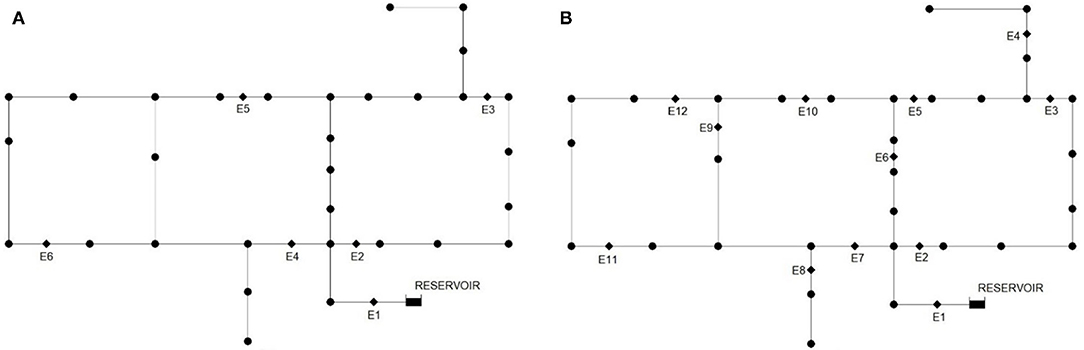
Figure 1. (A) Case #1: Modified hanoi network including six emitter nodes; (B) Case #2: Modified hanoi network including 12 emitter nodes.
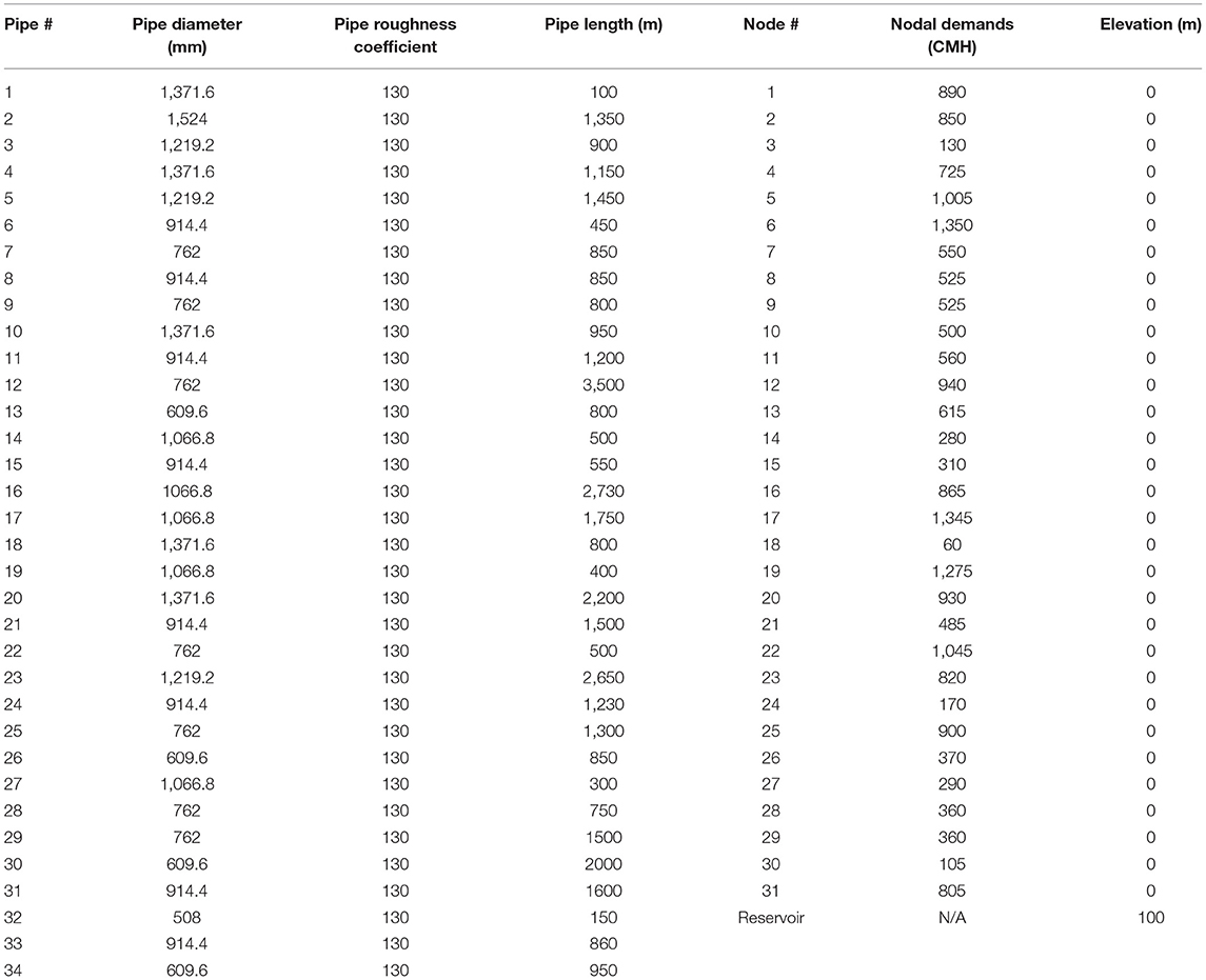
Table 1. Hanoi geometric and hydraulic specifications.
Leakage Induction Model
Emitters in EPANET 2.2 function as nodes which characterize the outflow through a nozzle or orifice discharging to the atmosphere (Muranho et al., 2014; Sebbagh et al., 2018). Such emitter nodes are associated with emitter coefficients that can be leveraged to model the severity of abovementioned outflows to the atmosphere (i.e., leakage). It is hypothesized that leakage has a direct correlation with pressure which can be characterized as the summation of background and bursts leakage (Muranho et al., 2014; Soldevila et al., 2016; Adedeji et al., 2017b; Zhou et al., 2019). The popular pressure-leakage relationship for a given pipe j can be shown as follows (Georgescu et al., 2017):
Where is the total discharge along pipe j in cubic meters per hour (cmh); lj is the length of pipe j in meters; αj and βj are parameters associated with background leakage model; Cj and γj are parameters of the bursts leakage model (EPANET 2.2 orifice formula); and Pj accounts for average pressure in pipe j in meters which equals the pressure at the emitter node k placed in the middle of pipe j. The background leakage term is considered zero in this paper, so the simplified EPANET-based leakage equation is as follows (Adedeji et al., 2017a):
Where is the total discharge along pipe j in cmh; Cj and γj are parameters of the bursts leakage model (i.e., Cj accounts for emitter coefficient at the emitter node placed in the middle of pipe j and γj is the emitter exponent that equals 0.5 by default in EPANET 2.2); and Pj accounts for average pressure in pipe j in meters which equals the pressure at the emitter node k placed in the middle of pipe j.
As the atmospheric discharge is deduced from Equation 2 at the emitter node (), the emitter actual demand in EPANET 2.2 equals the induced leakage discharge to the atmosphere, which signifies:
Where Dk accounts for the actual demand at emitter node k in cmh; and is the atmospheric discharge in cmh.
In order to characterize the amount of acceptable leakage at a given pipe, the absolute value of the proportion of atmospheric discharge at the emitter to the flow rate in the pipe comprising the emitter yields the amount of leakage percentage at the associated pipe. Equation 4 shows the leakage severity in percentage at pipe j:
Where is the leakage severity in percentage locally at pipe j; Dk accounts for actual demand at emitter node k in cmh; and denotes pipe-j inflow to emitter node k in cmh.
It is hereby postulated that the actual local leakage percentage at a given pipe is not meant to exceed a maximum value of 20% to only ensure the existence of major leaks rather than pipe breaks in Hanoi WDS.
Ultimately, in order to demonstrate the total leakage in the network, the following equation shows the network-wide leakage proportional to the total supply:
Where denotes the amount of leakage discharge in cmh (derived from Equations 2 and 3) to the atmosphere at emitter node j; j is the index for the emitter nodes; Qsup is the total supply of water to the WDS in cmh; and accounts for the network-wide leakage in percentage at emitter node j.
While inducing leakages in the two cases illustrated in Figure 1, it is hypothesized that the total amount of network-wide leakage () must not exceed a maximum of 10% to characterize a real-world scenario.
Prediction Model Formulation
In order to implement an optimization procedure for prediction purposes, genetic algorithms (GA) have been selected for (i) their robustness in meta-heuristically triangulating on a set of rather than a single solution point, (ii) high capability of being fine-tuned thanks to a decent number of algorithmic parameters, and (iii) a built-in constraint function that stands out compared structurally to Harmony Search or Particle Swarm algorithms. The prediction model is established upon the prediction of emitter coefficients (E) at the given places in two cases of actual leakage induction presented in Figure 1 by minimizing the objective function in the GA optimization framework. The objective function is composed of the mean squared error (MSE) of pressure values at the pressure monitoring locations.
Decision Variables
Emitter Coefficients (E) constitute the decision variables of the optimization framework and the set for E is as follows:
Where, e is the emitter coefficient for each of the given emitter nodes, and x is the number of considered emitter nodes in the WDS.
Objective Function
Pressure (Pk) measured at various pressure monitoring stations in the Hanoi water distribution network for a given set (k) of nodal demands (Qk) are characterized as follows:
Where, q is the nodal demand, y is the number of nodes in the WDS, p is the pressure measured at monitoring stations located in the WDS, and m is the number of pressure monitoring stations (PMSs) placed in the WDS.
The genetic algorithm optimization framework is utilized to predict the set E using j sets of Qk and Pk. For candidate (i) solution sets of E in the optimization process, pressures at the monitoring stations can be estimated as follows assuming all the dynamic condition parameters are known except for emitter coefficients:
Where, g() denotes the hydraulic simulations that could usually be conducted through software applications such as EPANET 2.2, Ei is a candidate solution set of emitter coefficients, i is the candidate solution reference in the optimization algorithm, and Pk,i is the estimated set of pressure values at all the monitoring stations for the corresponding candidate solution set Ei.
The objective function in the optimization algorithm is to minimize Z whereby,
Where a is the index for the pressure monitoring station, pa,k,i is the estimated pressure at PMS a for set of nodal demands k for candidate solution i, and pa,k is the actual measured pressure at PMS a for set of nodal demands k (obtained from set Pk).
Constraints
Three different constraints are employed in the proposed optimization model: (1) The minimum pressure head at all the nodes has to be >30 m for any candidate solution to be considered feasible; (2) Ensuring that none of the leakage flows at any of the emitter nodes would exceed a maximum value of 600 m3/h (cmh) based on Equations 2 and 3 (so as to avoid solutions with excessively high leakage flows); and (3) Constraining the maximum value of the local leakage ( from Equation 4) at each of the emitter nodes to a value of 20% (so as to avoid ridiculously large leaks).
Algorithmic Parameters
Efforts were made to tune the GA parameters according to the number of decision variables, complexity of the prediction model, constraint features, and time-efficiency. Table 2 shows these GA parameters specified for the proposed model in this study.

Table 2. Genetic algorithm parameters for both cases of actual leakage induction.
Characterization of Artificial Neural Networks (ANNs)
According to Figure 1, since there exist two cases of actual leakage induction, thus two separate but identical series of neural networks are trained to predict pressures at all the PMS locations for given sets of nodal demands and emitter coefficients so as to bypass the time-consuming application of EPANET 2.2 simulator toolkit in MATLAB. Table 3 displays the properties of ANNs used in MATLAB to train the simulated data by employing resilient backpropagation function (Riedmiller and Braun, 1993) for optimization framework.
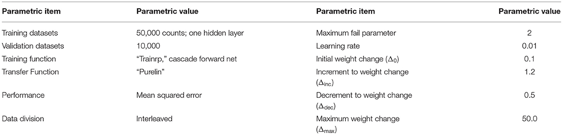
Table 3. Artificial neural networks parameters for both cases of actual leakage induction.
Formulation for Accuracy Measurement
This section offers accuracy metrics to analyze the performance of both trained neural networks and the prediction model numerically.
Neural Networks Accuracy Metric
The accuracy of trained neural networks (ANNs) is measured using a metric known as mean absolute percentage error (MAPE) (de Myttenaere et al., 2016; Khair et al., 2017) and is characterized as (Momeni and Piratla, 2021):
Where pri,j is the predicted value of pressure using the trained ANN model for node j in validation scenario i, simi,j is the simulated value of pressure calculated using EPANET 2.2 for node j in validation scenario i, y is the number of nodes in the WDS, and l is the number of the validation scenarios.
Prediction Model Accuracy Metric
The prediction model accuracy is also calculated both by employing Pearson's correlation coefficient formula (PCC) (Kumar and Jena, 2020) and MAPE similar to previous section, both characterized as follows:
Where, pri is the predicted value of either emitter coefficient for emitter i or the leakage severity (see Equations 2 and 3) for the associated pipe in the middle of which emitter i is placed, acti is the actual value of either the emitter coefficient for emitter i or the leakage severity (see Equations 2 and 3) for the associated pipe in the middle of which emitter i is placed, i denotes the index for emitter node, accounts for the average of either all actual emitter coefficients or all actual leakage severities across all the considered leakage-induced pipes, accounts for the average of either all predicted emitter coefficients or all predicted leakage severities across all the considered leakage-induced pipes, and x is either the number of the considered emitter nodes or the number of considered leakage-induced pipes in the WDS.
Where prj is the predicted value of either emitter coefficient for emitter j or the leakage severity (qleak) (see Equations 2 and 3) for the associated pipe in the middle of which emitter j is placed, actj is the actual value of either emitter coefficient for emitter j or the leakage severity (qleak) (see Equations 2 and 3 for the associated pipe in the middle of which emitter j is placed, y is either the number of the considered emitter nodes or the number of considered leakage-induced pipes in the WDS.
Results and Discussion
Proof-of-Concept Demonstration
This section accounts for the demonstration of leakage prediction through the proposed data-driven asset management scheme by exemplifying two separate cases of actual leakage locations: (i) leakage at six orifice nodes and (ii) leakage at 12 orifice nodes. For each of these two cases, a single scenario of partial consumption data and random placement of pressure monitoring stations (PMSs) in Hanoi WDS is established for a partial input-output (I/O) data of 70% of nodal demands and eight pressure stations in order to analyze the accuracy, robustness, and reliability of the proposed leakage model. In other words, it is assumed that it would be possible to obtain nodal demands from 70% of Hanoi WDS's nodes through the use of some nominal smart water meters and that there would be eight pressure monitoring sensors placed in the Hanoi WDS that would gather and relay pressure data synchronously with the nodal demand data. After generating 200 (j in Equation 9) demand scenarios to represent data from smart meters and corresponding pressure data from the eight pressure monitoring stations, artificial neural networks (ANN) are trained to mimic and replace the EPANET 2.2 hydraulic simulator in MATLAB for optimization purposes by employing genetic algorithms. The input data for these neural networks includes 70% of actual demand data (nodal demands) along with emitter coefficients (representing the leakage) and output data includes pressure values harvested from eight various smart meters across Hanoi network to establish the objective function (mean square error of actual and simulated pressures) in the optimization framework. Moreover, another set of neural networks is trained for leakage constraint as mentioned in the methodology section. Input data for ANN in this case includes the aforementioned partial demand sets and emitter coefficients, and ANN target data includes actual demands at emitter coefficients as well as inflow rates at the pipe preceding the emitter orifices (see Equation 4). Table 4 shows the specifics of ANN models along with the selected input and output data for the baseline scenario according to Hanoi WDS depicted in Figure 1.
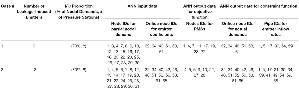
Table 4. Baseline scenario specifics of input and output data for the leakage model.
Neural Network Accuracy and Performance Analysis
The accuracy of the trained neural networks for pressure and leakage (composed of actual demands at emitter nodes and inflow rates, which is consequently calculated by Equation 4) using MAPE metric can be observed in Table 5.

Table 5. ANN MAPE values for baseline scenarios of the two cases.
Figures 2, 3 also demonstrate the performance analyses of training the neural networks for Case #1 and Case #2 respectively.
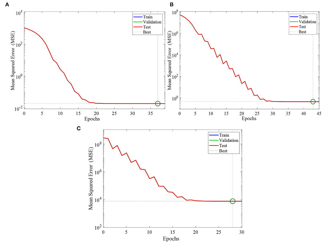
Figure 2. Performance analysis of Case #1 for (A) Pressure data training, (B) Actual demand data training, and (C) Flow data training.
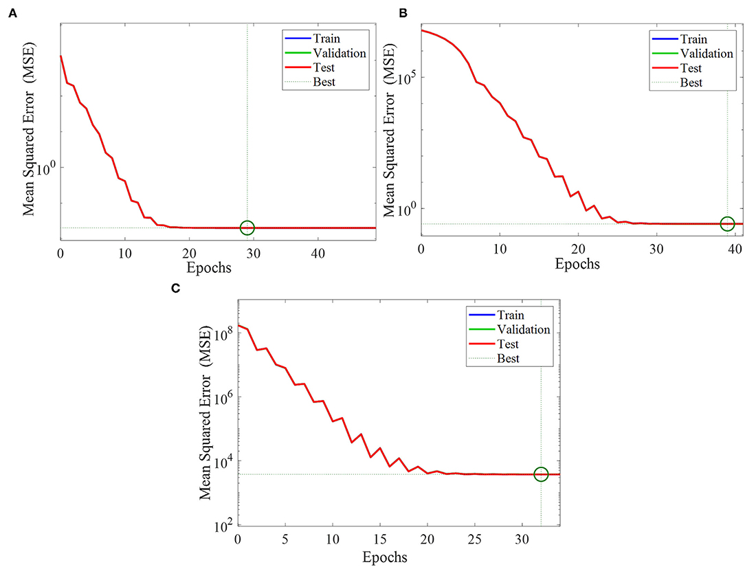
Figure 3. Performance analysis of Case #2 for (A) Pressure data training, (B) Actual demand data training, and (C) Flow data training.
According to the MAPE values in Table 5, these neural networks are reasonably accurate and appropriate alternatives for the EPANET 2.2 simulator toolkit in MATLAB, thus providing much higher time-efficiency for the execution of the prediction model and thus allowing the inclusion of thousands of scenarios for sensitivity analyses of placement and number of consumption data later in the paper.
Prediction Model Accuracy
The accuracy of the prediction model is measured using both Pearson's correlation coefficient (see Equation 11) and MAPE metric (see Equation 12) by considering the actual and predicted emitter coefficients (E) as well as the actual and predicted leakage severities (qleak). Figures 4, 5 illustrate the variation of actual and predicted emitter coefficients as well as actual and predicted leakage severities in cubic meters per hour (CMH) in Hanoi WDS for the two cases of leakage induction presented earlier.
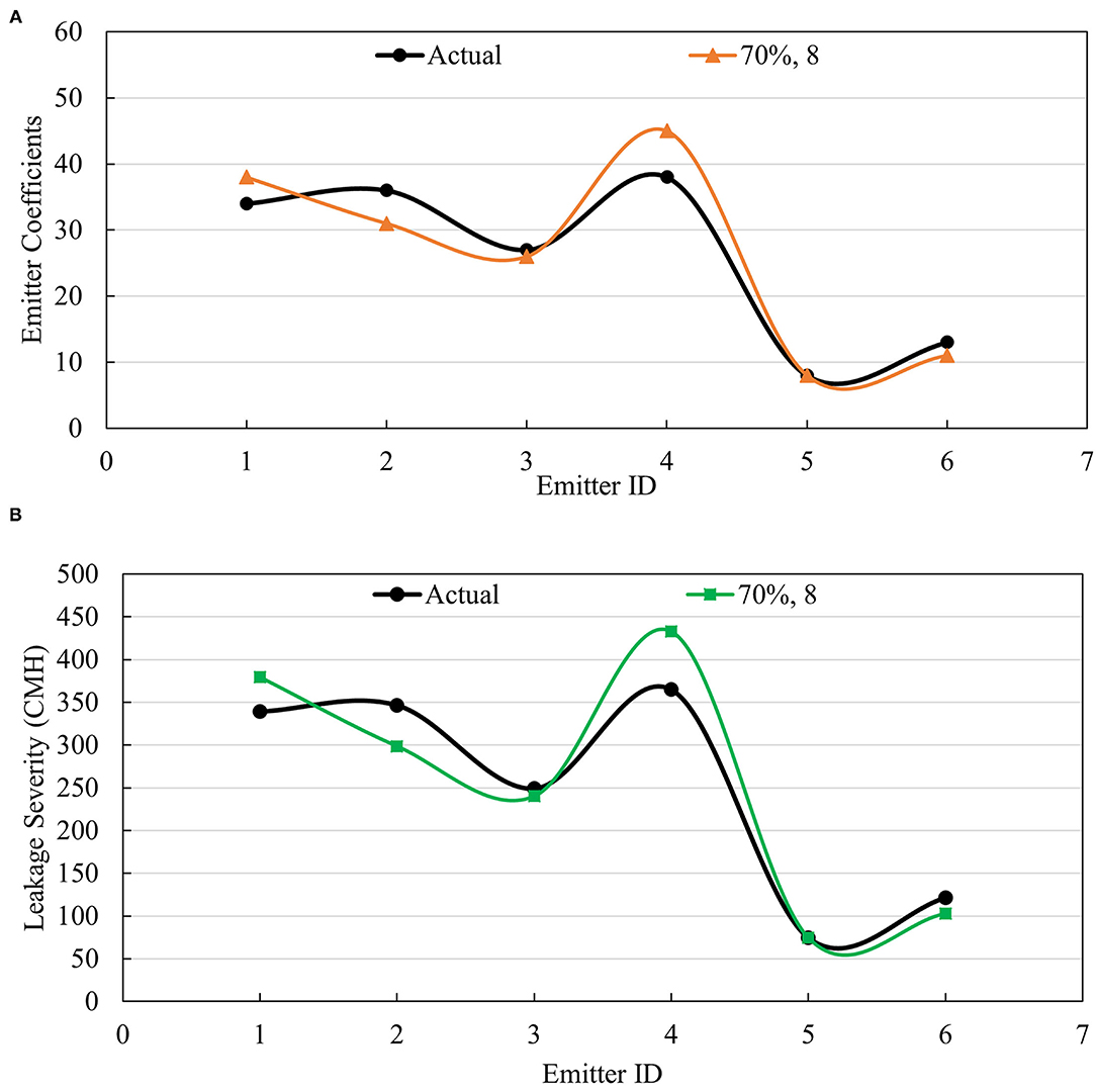
Figure 4. (A) Actual and predicted values of emitter coefficients of the baseline scenario for Case #1; (B) Actual and predicted values of leakage severity of the baseline scenario for Case #1.

Figure 5. (A) Actual and predicted values of emitter coefficients for Case #2; (B) Actual and predicted values of leakage severity for Case #2.
The Pearson's correlation coefficient (PCC) and MAPE value for the variation of emitter coefficient and leakage severities for both cases presented in Figures 4, 5 can be observed in Table 6. As can be viewed in Table 6, the actual and predicted values of emitter coefficients are found to be reasonably correlated. It can be observed that as the number of emitter coefficients increases from 6 to 12, the accuracy of the model will be affected and thus more sensitive to the variations of pressure in the objective function, which emphasizes the importance of sensitivity analyses presented later in the paper.

Table 6. Prediction accuracy values for emitter coefficients and leakage severity both cases.
Sensitivity Analyses
The sensitivity of the proposed leakage model to the placement and number of selected consumption nodes and pressure monitoring stations (PMSs) is measured by including 4,000 scenarios where various numbers of partial nodal demand datasets (i.e., ANN input data) and pressure monitoring stations (PMSs) (i.e. ANN output data) are randomly generated. Four categories of scenarios are developed for the sensitivity analyses, as identified in Table 7: (a) consumption data from 70% of demand nodes and pressure monitoring stations placed at eight locations, characterized as (70%, 8)—which is consistent with the baseline scenario discussed in the previous section; (b) (70%, 5), (c) (50%, 8), and (d) (50%, 5). 1,000 scenarios were randomly generated for each of these four categories out of which 100 scenarios were selected for sensitivity analyses based on the best ANN MAPE prediction for WDS pressure output data.
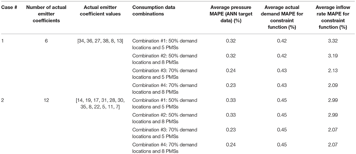
Table 7. Sensitivity analysis of trained neural networks for number and placement of consumption data meters for 4,000 scenarios.
Neural Networks Performance Analysis
As mentioned before, four separate categories of partial consumption data are studied to render the presented model more representative of the real-world data which can be harvested for modeling purposes. Table 7 depicts the specifics of generated scenarios for four different sets of input and output data associated with the previously discussed two different actual leakage cases in Hanoi WDS. As can be observed in Table 7, the MAPE values of trained neural networks for pressures as target data and leakage as data for constraint function averaged across the 4,000 scenarios of each of the two presented cases are found to be reasonably accurate in order to be fed into the optimization framework. According to Table 7, the average pressure MAPE as the ANN output tends to decrease as the number of consumption nodes is increasing from 50% of nodal demands and five pressure meters to 70% of nodal demands and eight pressure meters. This still holds true for the average inflow rate MAPE as it drops from 3.32 to 2.09% in Case #1 and 2.99 to 2.07% in Case #2. However, the average actual demand MAPE at emitter nodes is found to insignificantly increase for both cases. By comparing the average of all three averages for each combination of consumption data, it can be found that Case #2 demonstrates a slightly better accuracy than Case #1.
Prediction Model Accuracy Analysis
As mentioned before, the prediction model is applied to the best 100 scenarios (according to the best ANN MAPEs for pressure output) out of the 1,000 trained scenarios for each of the four categories described in the previous section for both of the cases. The accuracy of the prediction model in the sensitivity analyses section is also measured using MAPE metric and Pearson's Correlation Coefficient (PCC) (see Equations 11 and 12). Figures 6, 7 represent the emitter coefficient and leakage severity MAPE and PCC variations for the baseline scenarios along with each of the four sensitivity analyses categories (see Table 7). According to Figures 6, 7, it is noteworthy that the PCC and MAPE values in each of the cases are almost similar for emitter coefficients and leakage severity, since they are directly correlated according to Equation 2. Two types of comparisons are made according to Figures 6, 7: case-wise and pairwise.

Figure 6. (A) Case-#1 Accuracy metric variations with the number and locations of smart meters: (A) Emitter coefficient PCC; (B) Emitter coefficient MAPE; (C) Leakage severity PCC; (D) Leakage severity MAPE.
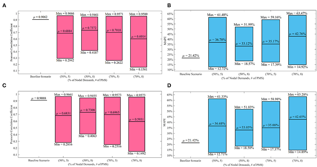
Figure 7. Case-#2 accuracy metric variations with the number and locations of smart meters: (A) Emitter coefficient PCC; (B) Emitter coefficient MAPE; (C) Leakage severity PCC; (D) Leakage severity MAPE.
Case Wise Comparison
This section compares the accuracy metrics in Case #1 to those in Case #2, as the number of emitter nodes increases.
Firstly, according to Figures 6, 7, it can be inferred that Case #2 displays a lower average prediction accuracy than Case #1 (average MAPE of ~12% in Case #1 compared to that of ~37% in Case #2 in all combinations) as the number of emitter nodes increases. This observation is consistent with the baseline scenario analysis in the proof-of-concept demonstration as well. It can also be concluded that the overall variations of both accuracy metrics range from 0.5306 to 0.9985 for PCC and from 1.98 to 30.94% for MAPE in Case #1 as well as from 0.1561 to 0.9666 for PCC and 12.72 to 63.47% for MAPE in Case #2. These relatively large ranges are indicative of the high sensitivity of the model to the number and locations of the selected smart meters for pressure and nodal demands across the network.
Pairwise Comparison
In this section, comparisons are made within each of the two cases in terms of the four categories (combinations) of partial nodal demands and pressure monitoring stations (Combinations #1 through #4 according to Table 7) for both emitter coefficient and leakage severity predictions.
Regarding Case-#1 emitter coefficient predictions, according to Figures 6A,B, the average PCC and average MAPE values for all the combinations range within 0.0099% and 0.22% respectively, which suggests that increasing the number of smart meters for wider consumption data combined with increased number of pressure monitoring stations does not necessarily contribute to greater average accuracy of the model for Case #1 with six leak sources across the network. Furthermore, comparing the prediction accuracy of Combinations #1 and #2 for Case #1 in Figure 6, the following observations can be made for when the number of pressure monitoring stations are increased from 5 to 8 keeping the percentage nodal input consideration at 50%: (1) the average PCC value drops from 0.9127 to 0.9060, which suggests that there is slightly less correlation among actual and predicted leakages although the number of pressure meters has increased. On the other hand, the average MAPE has slightly improved from 12.08% to 12.04%; (2) the maximum PCC value increased very marginally from 0.9976 to 0.9985, which is not a considerable improvement; (3) the least MAPE declined from 3.34% to 2.32%, which is also not greatly significant; and (4) the range of variation in PCC has shrunk going from Combination #1 to Combination #2 whereas it expanded for MAPE. Similar observations can also be made for the comparison of Combinations #3 and #4 where the number of pressure monitoring stations increased from 5 to 8 while the percentage nodal input consideration is at 70%. It can be concluded from these observations that increasing the number of pressure monitoring stations does not necessarily result in considerably better prediction accuracy of leakage severity assessment. On other hand, by comparing Combination #1 with Combination #3, it can be observed that (i) the average PCC and MAPE values show insignificant improvements as the percentage of nodal demands increases from 50% to 70%, while pressure meters remain constant; (ii) the minimum values of PCC and MAPE have improved from 0.5306 to 0.5765 and from 3.34% to 2.01% respectively; (iii) the maximum values of PCC and MAPE remain almost unchanged. Similarly, for Combinations #2 and #4, it can be observed that (i) the minimum and average PCC and MAPE values remain constant while the maximum values of MAPE show some improvement from 30.94% to 25.55%. This suggests that the inclusion of more nodal demands while considering 5 pressure stations does not necessarily improve the prediction accuracy, whereas the inclusion of more nodal demands while having 8 pressure stations slightly contribute to the sensitivity of the model. Similarly, the average values and variation ranges of the accuracy metrics for leakage severity in Figures 6C,D are identical to those of the emitter coefficients across the four combinations of sensitivity analyses. Based on the variation range of the prediction for all the categories studied in the sensitivity analyses, it can be concluded that optimizing the locations for placement of smart water meters and pressure monitoring stations in the WDS would yield the best prediction (i.e., highest PCC and lowest MAPE) of pipeline condition assessment as envisioned through the proposed approach.
Considering Case #2, as per Figures 7A,B, the average PCC and MAPE values with 12 emitter nodes for all four combinations are found to be within a range of 0.1358% and 9.64% respectively, which suggests that increasing the number of PMSs and the percentage of consumption data shows a more significant contribution compared to Case #1. It can thus be concluded that as the emitter nodes increase in number, the prediction model seems to show more sensitivity to the selected locations and numbers of the smart meters. Also, having the smallest MAPE variation range, Combination #2 demonstrates the lowest sensitivity of the model as well as the highest average accuracy (average MAPE equals 33.12%) out of all the four combinations. Furthermore, by comparing Combinations #1 and #2 from Figure 7, the following observations are noteworthy: (i) average PCC value improves from 0.6884 to 0.7372 and average MAPE value improves from 36.78% to 33.12%; (ii) the MAPE variation range shrinks from Combination #1 to Combination #2 as the minimum and maximum MAPE values change significantly. This significant change suggests increasing the number of pressure stations contributes to the performance of the model; (iii) although the maximum and mean PCC values show insignificant improvements from Combination #1 to Combination #2, the minimum PCC value improves considerably from 0.2942 to 0.4187. However, by comparing Combinations # 3 and #4, (i) the average PCC value deteriorates from 0.7018 to 0.6014 and the MAPE value worsens from 35.17% to 42.76%; (ii) the maximum and minimum PCC and MAPE values improve very inconsiderably. Overall, increasing pressure meters from 5 to 8 when 50% nodal demands is included is found to improve the model whereas the same scenario deteriorates the performance of the model when 70% nodal demands is leveraged. By comparing Combinations #1 and #3, it can be observed that (i) the average MAPE value demonstrate a marginal improvement; (ii) the minimum MAPE value is found to significantly worsen from 12.72% to 17.39%; (iii) the maximum MAPE value improves from 61.48% to 59.16%; (iv) the minimum, average, and maximum PCC values are found to have no significant changes. Similar comparisons between Combinations #2 and #4 suggest that (i) average PCC and MAPE values worsen significantly; (ii) minimum MAPE value improves from 18.57% to 14.92%, whereas the maximum MAPE value deteriorates from 51.99% to 63.47%; (iii) maximum PCC value remains almost constant while the minimum PCC value considerably drops from 0.4187 to 0.1561. As a result, it can be inferred that inclusion of more nodal demands at a constant number of pressure meters seems to have either minor or rather worsening effects on the accuracy of the model on average. Consistent with Case #1, the average values and variation ranges of the accuracy metrics for leakage severity in Figures 7C,D are identical to those of the emitter coefficients discussed in this paragraph across the four combinations of sensitivity analyses. Similar to Case #1, optimizing for locations to place smart water meters and pressure monitoring stations in the WDS would yield the best pipeline condition assessment prediction.
Conclusion and Future Work
This study aimed at proving the validity of a data-driven water pipeline leakage prediction scheme using artificial neural networks and genetic algorithms as demonstrated on Hanoi WDS. By employing pressure monitoring stations for a set of partial nodal demands, neural networks were trained and incorporated into a genetic algorithm optimization framework in MATLAB to predict emitter coefficients for two cases of actual leakage induction at six and 12 pipes respectively. The results indicate that (i) this preliminary prediction scheme offers promise to predict leakage severities based on cyber-monitoring data with reasonable accuracy and (ii) the prediction model does not show improvements when both consumption at more demand nodes and more pressure stations are considered, while on average the increase in the number of pressure stations at 50% nodal demands showed better accuracy and relatively higher correlation of parameters in the model for both cases. Some of the limitations of the study include (i) the consideration of leakage induction at some rather than all of the pipes, (ii) the assumption that leaking pipelines are known (locations of leaks were predefined), (iii) the assumption of the availability of consumption data collected synchronously with pressure data, (iv) the assumption that all other dynamic pipeline condition parameters (e.g., pipeline roughness, effective pipeline diameter) are known, and (v) the consideration of with high leakage outflows given the sizes of pipes in the Hanoi WDS. Future work should focus on: (1) prediction of leakages in all the pipelines without assuming that the leaking pipelines are known; (2) co-prediction of a variety of dynamic pipeline condition parameters including leakages, roughness values, effective hydraulic diameters, etc.; (3) wider validation campaign to cover WDSs of varying layouts and pipe sizes to test the ability of the proposed model in detecting smaller leakages; (4) optimizing the locations for placement of smart water meters and pressure monitoring stations in the WDSs for best pipeline condition prediction accuracy.
Data Availability Statement
The raw data supporting the conclusions of this article will be made available by the authors, without undue reservation and upon reasonable request.
Author Contributions
AM has completed coding and analyzing the results, as well as drafting the first version of this article. KP contributed toward strategizing the modeling approach in addition to providing inputs on broadening the impact of the results and its presentation in this article.
Funding
This research was supported by the National Science Foundation (NSF) under Grant No. 1638321. The authors are grateful to the NSF for this support.
Author Disclaimer
The results and conclusion presented in this paper are those of the authors and should not be interpreted as necessarily representing the official policies, either expressed or implied, of the United States Government.
Conflict of Interest
The authors declare that the research was conducted in the absence of any commercial or financial relationships that could be construed as a potential conflict of interest.
Publisher's Note
All claims expressed in this article are solely those of the authors and do not necessarily represent those of their affiliated organizations, or those of the publisher, the editors and the reviewers. Any product that may be evaluated in this article, or claim that may be made by its manufacturer, is not guaranteed or endorsed by the publisher.
References
Adedeji, K. B., Hamam, Y., Abe, B. T., and Abu-Mahfouz, A. M. (2017a). Burst leakage-pressure dependency in water piping networks: Its impact on leak openings. IEEE AFRICON: Sci. Tech. Innov. Afr. 1502–1507. doi: 10.1109/AFRCON.2017.8095704
Adedeji, K. B., Hamam, Y., Abe, B. T., and Abu-Mahfouz, A. M. (2017b). Towards achieving a reliable leakage detection and localization algorithm for application in water piping networks: an overview. IEEE Access 5, 20272–20285. doi: 10.1109/ACCESS.2017.2752802
Al Qahtani, T., Yaakob, M. S., Yidris, N., Sulaiman, S., and Ahmad, K. A. (2020). A review on water leakage detection method in the water distribution network. J. Adv. Res. Fluid Mech. Therm. Sci. 68, 152–163. doi: 10.37934/ARFMTS.68.2.152163
Creaco, E., and Haidar, H. (2019). Multiobjective optimization of control valve installation and DMA creation for reducing leakage in water distribution networks. J. Water Resourc. Plann. Manage. 145:04019046. doi: 10.1061/(asce)wr.1943-5452.0001114
De Marchis, M., and Milici, B. (2019). Leakage estimation in water distribution network: effect of the shape and size cracks. Water Resourc. Manage. 33, 1167–1183. doi: 10.1007/s11269-018-2173-4
de Myttenaere, A., Golden, B., Le Grand, B., and Rossi, F. (2016). Mean absolute percentage error for regression models. Neurocomputing 192, 38–48. doi: 10.1016/j.neucom.2015.12.114
Fujiwara, O., and Khang, D. B. (1990). A two-phase decomposition method for optimal design of looped water distribution networks. Water Resourc. Res. 26, 539–549. doi: 10.1029/WR026i004p00539
Gao, Y., Brennan, M. J., Liu, Y., Almeida, F. C. L., and Joseph, P. F. (2017). Improving the shape of the cross-correlation function for leak detection in a plastic water distribution pipe using acoustic signals. Appl. Acoustics 127, 24–33. doi: 10.1016/j.apacoust.2017.05.033
Georgescu, A. M., Perju, S., Madularea, R. A., and Georgescu, S. C. (2017). Energy consumption due to pipe background leakage in a district water distribution system in bucharest. Proc. Int. Conf. Energ. Environ. Energy Saved Today Asset Fut. 2017, 251–254. doi: 10.1109/CIEM.2017.8120785
Grigg, N. S. (2017). Water supply pipeline failures: investigative procedures and data management. J. Perform. Constr. Fac. 31:06017004. doi: 10.1061/(asce)cf.1943-5509.0001113
Gupta, A., and Kulat, K. D. (2018). A selective literature review on leak management techniques for water distribution system. Water Resourc. Manage. 32, 3247–3269. doi: 10.1007/s11269-018-1985-6
Hu, X., Han, Y., Yu, B., Geng, Z., and Fan, J. (2021). Novel leakage detection and water loss management of urban water supply network using multiscale neural networks. J. Clean. Produc. 278, 123611. doi: 10.1016/j.jclepro.2020.123611
Khair, U., Fahmi, H., Hakim, S., and Al Rahim, R. (2017). Forecasting error calculation with mean absolute deviation and mean absolute percentage error. J. Phy. Conf. Series 930:2002. doi: 10.1088/1742-6596/930/1/012002
Kumar, G. P., and Jena, P. (2020). Pearson's correlation coefficient for islanding detection using micro-PMU measurements. IEEE Syst. J. 1–12. doi: 10.1109/jsyst.2020.3021922
Liu, Y., Ma, X., Li, Y., Tie, Y., Zhang, Y., and Gao, J. (2019). Water pipeline leakage detection based on machine learning and wireless sensor networks. Sensors 19, 1–21. doi: 10.3390/s19235086
Ma, Y., Gao, Y., Cui, X., Brennan, M. J., Almeida, F. C. L., and Yang, J. (2019). Adaptive phase transform method for pipeline leakage detection. Sensors 19:310. doi: 10.3390/s19020310
Momeni, A., and Piratla, K. R. (2021). Leveraging hydraulic cyber-monitoring data to support primitive condition assessment of water mains. ASCE J. Pipeline Syst. Eng. Pract. doi: 10.1061/(ASCE)PS.1949-1204.0000596
Momeni, A., Piratla, K. R., and Madathil, K. C. (2020). “A novel computationally efficient asset management framework based on monitoring data from water distribution networks,” in Construction Research Congress 2020: Infrastructure Systems and Sustainability—Selected Papers from the Construction Research Congress 2020, 370–379.
Momeni, A., Prasad, V., Dharmawardena, H. I., Piratla, K. R., and Venayagamoorthy, K. (2018). “Mapping and modeling interdependent power, water, and gas infrastructures,” in Clemson University Power Systems Conference, PSC 2018.
Muranho, J., Ferreira, A., Sousa, J., Gomes, A., and Sá Marques, A. (2014). Pressure-dependent demand and leakage modelling with an EPANET extension—WaterNetGen. Proc. Eng. 89, 632–639. doi: 10.1016/j.proeng.2014.11.488
Piratla, K. R., and Momeni, A. (2019). “A novel water pipeline asset management scheme using hydraulic monitoring data,” in Pipelines 2019: Multidisciplinary Topics, Utility Engineering, and Surveying—Proceedings of Sessions of the Pipelines 2019 Conference. 190–198.
Riedmiller, M., and Braun, H. (1993). A direct adaptive method for faster background learning, the RPROP algorithm. Proc. Int. Conf. Neural Netw. 586–591. doi: 10.1109/ICNN.1993.298623
Sebbagh, K., Safri, A., and Zabot, M. (2018). Pre-Localization approach of leaks on a water distribution network by optimization of the hydraulic model using an evolutionary algorithm. Proceedings 2:588. doi: 10.3390/proceedings2110588
Shukla, H., and Piratla, K. (2020). Leakage detection in water pipelines using supervised classification of acceleration signals. Autom. Constr. 117:103256. doi: 10.1016/j.autcon.2020.103256
Soldevila, A., Blesa, J., Tornil-Sin, S., Duviella, E., Fernandez-Canti, R. M., and Puig, V. (2016). Leak localization in water distribution networks using a mixed model-based/data-driven approach. Control Eng. Pract. 55, 162–173. doi: 10.1016/j.conengprac.2016.07.006
Sophocleous, S., Savi,ć, D., and Kapelan, Z. (2019). Leak localization in a real water distribution network based on search-space reduction. J. Water Resourc. Plann. Manage. 145:04019024. doi: 10.1061/(asce)wr.1943-5452.0001079
Xie, X., Hou, D., Tang, X., and Zhang, H. (2019). Leakage identification in water distribution networks with error tolerance capability. Water Resourc. Manage. 33, 1233–1247. doi: 10.1007/s11269-018-2179-y
Yazdekhasti, S., Piratla, K. R., Sorber, J., Atamturktur, S., Khan, A., and Shukla, H. (2020). Sustainability analysis of a leakage-monitoring technique for water pipeline networks. J. Pipeline Syst. Eng. Pract. 11:425. doi: 10.1061/(ASCE)PS.1949-1204.0000425
Zhang, K., Yan, H., Zeng, H., Xin, K., and Tao, T. (2019). A practical multi-objective optimization sectorization method for water distribution network. Sci. Total Environ. 656, 1401–1412. doi: 10.1016/j.scitotenv.2018.11.273
Zhang, W., Huang, Z., Dasmeh, A., Yu, P., and Taciroglu, E. (2018). “Soil-structure interaction and failure analyses of steel water pipelines with welded joints,” in 11th National Conference on Earthquake Engineering 2018, NCEE 2018: Integrating Science, Engineering, and Policy 7, 3954–3963.
Zhou, X., Tang, Z., Xu, W., Meng, F., Chu, X., Xin, K., et al. (2019). Deep learning identifies accurate burst locations in water distribution networks. Water Res. 166:115058. doi: 10.1016/j.watres.2019.115058
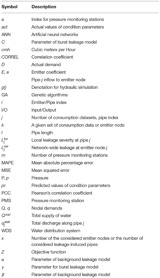
Nomenclature
Keywords: pipeline condition assessment, pipeline leak detection, smart utilities, pipeline monitoring system, evolutionary optimization
Citation: Momeni A and Piratla KR (2021) A Proof-of-Concept Study for Hydraulic Model-Based Leakage Detection in Water Pipelines Using Pressure Monitoring Data. Front. Water 3:648622. doi: 10.3389/frwa.2021.648622
Received: 01 January 2021; Accepted: 19 July 2021;
Published: 12 August 2021.
Edited by:
Elnaz Peyghaleh, Independent Researcher, Columbia, United StatesReviewed by:
Ramakrishna Tipireddy, Pacific Northwest National Laboratory, United StatesGreta Vladeanu, Xylem, United States
Copyright © 2021 Momeni and Piratla. This is an open-access article distributed under the terms of the Creative Commons Attribution License (CC BY). The use, distribution or reproduction in other forums is permitted, provided the original author(s) and the copyright owner(s) are credited and that the original publication in this journal is cited, in accordance with accepted academic practice. No use, distribution or reproduction is permitted which does not comply with these terms.
*Correspondence: Kalyan R. Piratla, a3BpcmF0bEBjbGVtc29uLmVkdQ==