 Wen-Ping Tsai
 Kuai Fang
 Xinye Ji1,3
94% of researchers rate our articles as excellent or good
Learn more about the work of our research integrity team to safeguard the quality of each article we publish.
Find out more
ORIGINAL RESEARCH article
Front. Water, 27 November 2020
Sec. Water and Hydrocomplexity
Volume 2 - 2020 | https://doi.org/10.3389/frwa.2020.583000
This article is part of the Research TopicBroadening the Use of Machine Learning in HydrologyView all 10 articles
Some machine learning (ML) methods such as classification trees are useful tools to generate hypotheses about how hydrologic systems function. However, data limitations dictate that ML alone often cannot differentiate between causal and associative relationships. For example, previous ML analysis suggested that soil thickness is the key physiographic factor determining the storage-streamflow correlations in the eastern US. This conclusion is not robust, especially if data are perturbed, and there were alternative, competing explanations including soil texture and terrain slope. However, typical causal analysis based on process-based models (PBMs) is inefficient and susceptible to human bias. Here we demonstrate a more efficient and objective analysis procedure where ML is first applied to generate data-consistent hypotheses, and then a PBM is invoked to verify these hypotheses. We employed a surface-subsurface processes model and conducted perturbation experiments to implement these competing hypotheses and assess the impacts of the changes. The experimental results strongly support the soil thickness hypothesis as opposed to the terrain slope and soil texture ones, which are co-varying and coincidental factors. Thicker soil permits larger saturation excess and longer system memory that carries wet season water storage to influence dry season baseflows. We further suggest this analysis could be formulated into a data-centric Bayesian framework. This study demonstrates that PBM present indispensable value for problems that ML cannot solve alone, and is meant to encourage more synergies between ML and PBM in the future.
Basin water storage has deep connections with streamflow (Reager et al., 2014; Fang and Shen, 2017). Hence terrestrial water storage anomalies (TWSA) data could, under certain circumstances, be used to increase flood forecast lead time (Reager et al., 2015). From a physical hydrologic point of view, more water stored in a basin could mean a higher groundwater table or wetter soils which lead to more runoff source areas (Dingman, 2015). The storage-streamflow relationship is also important for predicting baseflow (Thomas et al., 2013) and related ecosystem (Poff and Allan, 1995) and water supply issues. The issue is that these relationships vary widely in space. Fang and Shen (2017) (hereafter named FS17, more description in section The Background Story) conducted an analysis of the correlation between TWSA annual extrema and different streamflow percentiles in a year, and found very interesting patterns of these correlations over the conterminous United States (CONUS). The correlations between TWSA annual extrema and high-percentile flows are strong in certain parts of the CONUS, e.g., the southeastern Coastal Plain and northern Great Plains, but are weak in other areas such as the Appalachian Plateau, northern Indiana, and Florida. Why are there wildly different storage-streamflow relationships, i.e., what physical factors caused them? Our limited understanding of this question hampered our use of water storage and groundwater data in flood forecasting.
In general, to answer “why” questions such as the one raised above, one could resort to two avenues: process-based models (PBMs) or data-driven analyses. They are often regarded as two separate roads that do not cross. PBMs embody our beliefs about how the system functions. We can use PBMs to conduct numerical experiments to assess causal relationships, as we can alter measurable physical factors to directly examine their impacts on the outputs. We typically employ a “model-centric” framework, where we (i) deploy some prior distributions or beliefs of model structures; (ii) create an ensemble of model simulations (with different parameter sets, inputs, or model structures); (iii) confront these models with observations by evaluating likelihood functions either formally or informally by visually examining the outcomes; and (iv) identify the model(s) that best describe(s) the data. It is easy to see that paradigms like model calibration (Vrugt et al., 2003) or Monte Carlo Markov Chain (Vrugt et al., 2009) fit into this framework. Moreover, numerical experiments where the modelers perturb model physics on an ad-hoc basis (e.g., Maxwell and Condon, 2016; Shen et al., 2016; Ji et al., 2019) could also be placed in this framework. Potential issues with this framework are that it can be both subjective and inefficient, as many competing hypotheses remain un-tested. The priors are often based on one's own beliefs, and one needs to throw a huge amount of simulations to capture the plausible model structure. It has been argued that hydrologic models are necessarily degenerate (Nearing et al., 2016) and even sampling exhaustively from its parameter distribution does not capture the whole possible model space.
In contrast to PBMs, various interpretable machine learning approaches could be used to generate possible explanations, or “hypotheses” in machine learning language (Russell and Norvig, 2009), of an observed behavior. For example, the weights from linear regression could inform us of the relative importance of factors. Classification and regression tree (CART) analysis (Breiman et al., 1984; Mitchell, 1997), which iteratively separates data points based on predictors and their thresholds, is another explanatory tool that has often been employed. For example, Verhougstraete et al. (2015) used the first level split in a CART model to draw the conclusion that septic systems are the primary driver of fecal bacteria levels in 64 US rivers. An advantage of machine learning approaches is that they are highly efficient to execute compared to PBMs, and the models they generate are already consistent with data. They also carry the appeal of relying less on subjective assumptions and model choices.
However, the “Achilles heel” for machine learning as an explanatory tool is arguably their inability to distinguish between causal and associated relationships. If we had a large enough training dataset that covered all possible combinations of physical factors, machine learning should theoretically be able to extract the causal factor. However, we are limited by the combinations that exist in the real world and for which we have data, posing limits on the power of data. Naturally, one might wonder if PBMs' strength in causality analysis could be exploited to complement machine learning algorithms.
Recently, there have emerged increasing interest in combining physics with data-driven models. One could adopt a variety of methods loosely termed “physics-guided machine learning” (PGML) or “theory-guided machine learning” (Ganguly et al., 2014; Karpatne et al., 2017; Jia et al., 2019; Read et al., 2019; Yang et al., 2019), such as modifying the loss function to accommodate physical constraints (Jia et al., 2019) or pre-training a ML model using PBM outputs (Jia et al., 2018). These constructive ideas have made ML more robust and have enriched our means of investigations. Nevertheless, PGML frameworks have not taken advantage of PBM's ability to conduct experiments and assess causes and effects. Here we propose that the evaluation of competing hypotheses could be accomplished by running numerical experiments with a PBM to utilize the physics encoded in the PBM (Figure 2), as an example of the alternative research avenue proposed earlier (Shen et al., 2018). We then compare the probability of each hypothesis and reject those with low probability. Bayes' law allows information from different sources to be merged in a sequential manner given some evidence. In the context of hydrology (Beven and Binley, 1992; Kavetski et al., 2006; Raje and Krishnan, 2012; Viglione et al., 2013), the gist is that a likelihood function based on (oftentimes subjective) assumptions of error or data distribution replaces the conditional probability of observing a data point given model parameters. While such kinds of likelihood functions have been well-established, Bayes' law itself is quite generic and not restricted to this use. An opportunity exists to explore using Bayes' law to use process-based models to provide a quantification of the likelihood. Because this framework first starts with data, we call it a data-centric framework, in contrast to a conventional model-centric Bayesian framework where a model's inputs and parameters are perturbed and the posterior probability of each realization is calculated. We will use the storage-streamflow question to showcase the effectiveness of this framework and help us understand the main controlling factors of streamflow in the Susquehanna River basin to inspire best modeling practices. This work is a first exploration of this particular method of coupling data-driven hypotheses with process-based modeling capabilities, and by no means do we indicate this method is optimal or the most efficient.
In the following, we first provide some background for the case study of streamflow-storage correlations and the competing hypotheses that explain them (section The Background Story). Then we describe the process-based model and the experimental setup (sections Process-Based Hydrologic Model and Competing Hypotheses and the Implementation of Perturbation Experiments). We make sure the model produces reasonable hydrologic dynamics (section Performance of the Physically-Based Model), and then finally we use the perturbation experiments to test the competing hypotheses from ML (section Testing Competing Hypotheses).
In FS17 we introduced a hydrologic signature termed the Storage-Streamflow-Correlation Spectrum (SSCS), which quantifies how water storage is correlated with streamflow at different flow regimes. SSCS is the collection of Pearson's correlation coefficients (R) between annual extrema (peaks or troughs) of the terrestrial water storage anomalies (TWSA) and different streamflow percentiles (15 percentiles extracted are: {0.5%, 1%, 2%, 5%, 10%, 20%, 50%, 60%, 70%, 80%, 90%, 95%, 98%, 99%, 99.5%}) in a window around the extrema for the same basin. The correlations are calculated on an annual scale, using the water year (the 12-month period from October 1 through September 30 of the following year). The study period of FS17 is from 1 October 2002 to 31 September 2012. Treating each flow percentile as a “band,” we obtained a correlation “spectrum.” The SSCS gives a snapshot of the correlations across all bands, as compared to previous studies that focused only on high flow regimes.
If streamflow is disconnected from storage, e.g., when most rainfall runs off or evaporates directly without entering the subsurface, the system would exhibit low correlation between flows and storage during peak flows. Generally, the high-flow bands have lower R than low-flow bands because peak streamflows result from large storms whose magnitudes are poorly correlated to water storage. In contrast, if groundwater exerts a significant influence over streamflow, we expect the correlation to be higher. A high correlation between TWSA peaks and low flows indicates a long system memory: when such basins receive plenty of precipitation in the wet season, the excess storage is carried over the seasons and is reflected in low flows. Therefore, SSCS gives us a window of observation into how varied surface and subsurface hydrologic systems function. Please see FS17 for more details.
When applying the SSCS over the conterminous United States (CONUS), a large variety of SSCS behaviors emerged (FS17). To facilitate our interpretation, we clustered these responses into 6 different classes using K-means and a distance measure (the Euclidean distance in the SSCS space). The correlation values for different classes and the spatial distribution of classes are shown in Figure 1. We can clearly observe regional clusters and spatial gradients in the SSCS patterns. Class #1 was described as “full-spectrum responsive” since it had the highest correlations and the smallest variability across all SSCS bands. Class #1 concentrated on the southeast Coastal Plain and northern Great Plains. Class #2 and #3 catchments had weaker SSCS values and were concentrated along the northern Appalachian Plateau. For Class #3, in peak-TWSA bands, streamflow-storage correlation was low for flow percentiles below 20%, but higher for percentiles above 60%; in trough-TWSA bands, there were high streamflow-storage correlations at percentiles below 60%, but correlations were a little lower for high streamflow percentiles (80% above). Class #2 can be considered a transition type between class #1 and class #3.
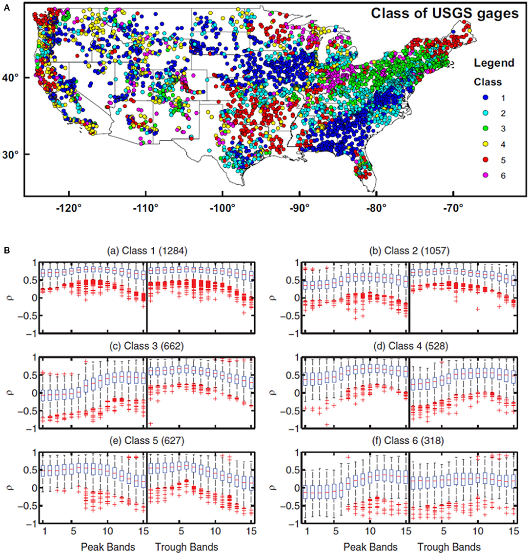
Figure 1. Class map (A) and boxplots of the SSCS for Class #1 to Class #6 (B). The boxes contain 25–75% percentiles, and the crosses are those considered outliers (Reprinted from FS17 with permission).
When observing the large spatial gradients of SSCS classes over CONUS in Figure 1, one cannot help asking, “what causes the SSCS behavior to differ between Appalachia and the Coastal Plain?”, which was the central question of this study. FS17 employed a CART analysis to learn simple and interpretable decision rules (the split criteria and thresholds) from the data. Focusing on the differences between basins in Appalachia (Appalachian Plateau, Piedmont, and Valley and Ridge physiographic provinces) and basins in the southeastern Coastal Plain, FS17 trained a specific CART model to predict the distances of basins to class centers in SSCS space. They used a number of predictors including the aridity index, depth to bedrock, rainfall seasonality, and the fraction of precipitation as snow (supporting information Table S1 in FS17). In other words, they asked what factors made the two clusters of basins different in terms of their SSCS patterns. From this ad hoc tree, the CART-based model automatically identified soil thickness (RockDep), obtained by merging soils-survey-based depth to bedrock with bedrock depth simulated by a geomorphological model (Pelletier et al., 2016) as the main difference between the two types of streamflow-storage correlation patterns.
The problem of learning an optimal CART is that a CART is not robust. This can be mitigated by training multiple trees in an ensemble as in the random forest (RF) algorithm (Ho, 1995), where the features and samples are randomly sampled with replacement. The RF generalizes from the CART and provides an estimation of probability. While RF models are more robust and can be used to infer probabilities, they are more difficult for humans to interpret.
While the RockDep explanation does make physical sense, it could be dangerous to take this hypothesis as the truth. First, even though soil thickness appeared to be the stronger explanatory model, there could be other slightly weaker but nonetheless valid models. We have yet to explore what would happen if we slightly alter the training dataset. Because we rely on available data, the results may be dependent on a few data points that critically cover certain parts of the input space. However, such critical data points may happen to be missing in our training data; the robustness of the model has not been established.
To answer our central question, here we propose a novel framework that combines the strengths of machine learning and process-based modeling. In this framework, machine learning first presents competing hypotheses and assigns them prior probabilities. Then, we construct numerical perturbation experiments with a process-based model to implement and test the hypotheses (Figure 2). The testing of the hypotheses could be achieved by visual examination of the outcome of the experiments, or via a more quantitative Bayesian approach.
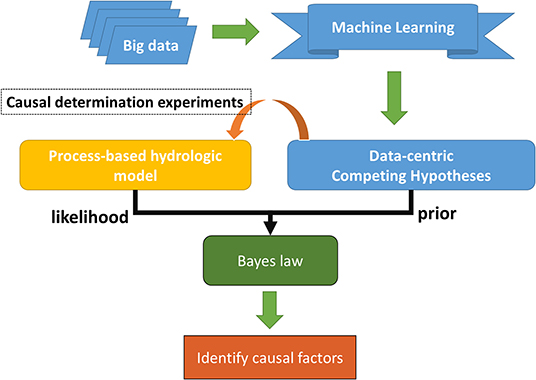
Figure 2. A framework for integrating PBM and machine learning.
The Susquehanna River (watershed area: 71,225 km2) is a major river located in the northeastern and mid-Atlantic United States (Figure 3A), which has historically been the source of many instances of flooding damage along the main river floodplains (Yarnal et al., 1997; May, 2011). The basin spans the physiographic provinces of the Appalachian Plateau, Piedmont, Valley and Ridge, and Coastal Plain regions. In general, most of the northern subbasins of the SRB consist of mountains mantled by thin soils which are mostly thinner than 2 m (Figure 3B). We show the SSCS behaviors of 13 randomly selected subbasins in the Susquehanna River Basin. We found that the all 13 stations in the Susquehanna River Basin belong to either Class #2 or Class #3 (Figure 3C, the original pattern of SSCS from 13 USGS gauge stations is similar to class #3).
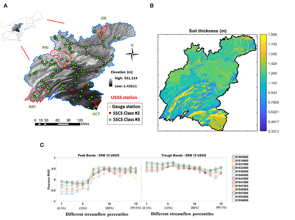
Figure 3. Study area, Susquehanna River Basin (SRB). Main class of SRB observation data is class #3 and #2 in FS17. (A) Study area, Susquehanna River Basin. Among the subbasins modeled, OR and PIN are headwater subbasins in the Appalachian Plateau, RAY is a headwater subbasin in the Valley and Ridge physiographic division, and OCT is near the Coastal Plain region. (B) Soil thickness. (C) SSCS in Susquehanna River Basin for 13 USGS gauge stations (station numbers in legend).
We further chose 4 subbasins (Figure 3A), namely, the Otselic River basin (OR), the Pine Creek basin (PIN), the Raystown Branch Juniata River basin (RAY), and the Octoraro Creek basin (OCT) in the south to create process-based hydrologic models. Both soils survey data and global modeled soil thickness data were used to parameterize soil thickness: in most of the basin where the bedrock is within the limit of the soils survey depth (1.52 m), the RockDep attribute in SSURGO (NRCS, 2010) was used; outside of these areas, we used the average soil and sedimentary layer thickness from Pelletier et al. (2016), which has global coverage with 1 km resolution. Among the subbasins modeled, OR and PIN are headwater subbasins in the Appalachian Plateau, RAY is a headwater subbasin in the Valley and Ridge physiographic division, and OCT is near the Coastal Plain region. OCT has a visibly larger soil thickness.
To be able to conduct causal experiments, we employed the Process-based Adaptive Watershed Simulator coupled with the Community Land Model (PAWS+CLM) (Shen and Phanikumar, 2010; Shen et al., 2013, 2014, 2016; Ji et al., 2015, 2019; Niu et al., 2017; Ji and Shen, 2018; Fang et al., 2019). First introduced in Shen and Phanikumar (2010), the PAWS model was coupled to the Community Land Model (CLM) (Collins et al., 2006; Dickinson et al., 2006; Oleson et al., 2010; Lawrence et al., 2011) which describes the land surface and vegetation dynamics (Shen et al., 2013). The PAWS model has been used to explain the relative importance of different controlling processes on hydrologic and ecosystem dynamics. CLM incorporates comprehensive physical and biogeochemical processes including vapor and momentum transfer, surface radiative transfer, soil heat transfer, freeze-thaw phase changes, and biochemical photosynthesis, as well as plant carbon and nitrogen cycles (Shen et al., 2014). PAWS+CLM inherits the land surface processes from CLM, including surface energy fluxes, ET, vegetation growth, and carbon cycling, while solving physically-based conservative laws for flow processes including 2D overland flow, quasi-3D subsurface (soil and groundwater) flow, vectorized channel networks, and the exchanges among these domains. The flow module starts with throughfall, stemflow, and snowmelt as the precipitation inputs, and converts the CLM-computed evapotranspiration term into a sink. The surface water layer is divided into the flow domain, which can flow laterally, and the ponding domain, which exchanges with the main soil column and does not circulate laterally. The flow domain water is routed downstream as overland flow, described by a diffusive wave equation (DWE). Infiltrated water is governed by the Richards equation. Water reaching the phreatic water table may move laterally, as described by Dupuit-Forchheimer flow in an unconfined aquifer. 1D columns of vertical soil flow are coupled to the saturated lateral flow at the bottom. The confined aquifers below are described by a 3D saturated groundwater flow equation. The channel flow is governed by DWE in a 1D cascade network. More information about PAWS can be found in Shen et al. (2016).
In this study, a 1,040 ×1,040 m horizontal grid was used to discretize the domain. Precipitation and climate forcing data used in PAWS+CLM were obtained from the North American Land Data Assimilation System (NLDAS) (Mitchell, 2004). Information from the Soil Survey Geographic Database (SSURGO) was used to provide initial values for the soil properties. In PAWS+CLM, we extracted topographic information from the National Elevation Dataset (30 m) to parameterize the river bed elevations, and used the mean elevation to parameterize the gridcell elevation (Shen et al., 2016). The climatic forcing datasets that come from NLDAS are on an hourly basis.
The channel network is represented by an explicit, vectorized channel network for larger rivers and the implicit, gridded overland flow for smaller headwater streams. As an advance of PAWS+CLM, the channel network topology is now established based on the National Hydrography Dataset Plus Version 2 (NHDPlus V2) shapefiles. In NHDPlus V2, each segment is encoded with a unique ID number and the downstream ID. Combing through this connectivity information, our pre-processing package traces the rivers from downstream to upstream and records the river distances of each segment. The available channels from NHD are vastly greater than what can be explicitly represented in the vectorized channel network in the model. In previous work, the selection of the explicitly modeled streams was manual. We have now implemented an automatic selection procedure: our pre-processing utility iteratively selects the longest rivers from the candidate pool built from NHDPlus V2, so that the total selected river length satisfies a prescribed river density (river length : basin area). Based on these explicitly represented rivers, we then establish a network structure, recording names of the streams, network topology, upstream/downstream nodes in the hierarchy, boundary condition types (headwater, inflow, connecting streams, or outflow), tributaries, and locations of confluences. For each explicitly modeled river, the discretization procedure evenly distributes the river polyline into river cells. We then overlay the river cell with high resolution DEM and groundwater data, extracting information, e.g., bank and bed elevation (inferred through regional regression equation), during discretization (Shen et al., 2016).
In PAWS the soil water retention and unsaturated hydraulic conductivity are parameterized using the van Genuchten formulation. To obtain spatially distributed van Genuchten parameters, we incorporated a range of well-established pedotransfer functions (PTFs) (Guber et al., 2009) and the Rosetta (Schaap et al., 2001) program which employs a hierarchy of PTFs, ranging in complexity from a soil textural lookup table to algorithms based on Artificial Neural Networks (ANN). We also exported soil textural information (sand, clay, and silt percentages), bulk density, and water contents from soil horizon data from the SSURGO database (NRCS, 2010) into Rosetta, wherever they were available. Rosetta was then used to predict van Genuchten parameters, and the results were subsequently read into PAWS. Normally, we chose the “best possible model” option in Rosetta. The SSURGO database contains fine resolution (1:24,000 map scale) soil type maps, which are encoded as “map unit” keys (mukey). A mukey value serves as an index key to the SSURGO relational databases that detail the characteristics of that soil type. A mukey may contain several “soil components,” each taking up a certain fraction of the map unit. Every component then describes the vertical soil horizons and their depths.
The runtime of PAWS-CLM for 18 years of simulation in an SRB subbasin (OR) is about 4 h on a machine with CPU. Even with the help of the pedotransfer functions, process-based hydrologic model parameters need to be further adjusted or calibrated. The SRB is large, and it is difficult to perform calibration for the whole basin. We thus defined our objective function as the mean of the Nash-Sutcliffe model efficiency coefficients (Nash and Sutcliffe, 1970) for the four subbasins. This way, the resulting parameter set may not produce the best achievable performance for each subbasin, but presents a balance between them for the whole basin. Model performance was evaluated against USGS streamflow records.
To identify potential competing hypotheses, we first ran a CART analysis, which combines classification tree and linear regression algorithms, for both southeastern and Appalachian basins with multiple random seeds and randomized removal of training data points (basins). A classification tree is used to split data points with a binary decision rule, and a linear regression is used to predict the distance to clusters' centroids. The runtime of the CART-based model was 3~5 s for both the southeastern and Appalachian areas. Then we further ran RF analysis with an expanded list of attributes. With the CART-based model, we considered all basin physiographic parameters that were deemed as important for SSCS in FS17, including: RockDep, sand, slope, soil bulk density, watershed percent agriculture, watershed percent developed, and standard deviation of elevation. In FS17, we employed sand and clay as representatives for soil texture and removed silt, since they add up to one. In the present analysis we also followed this practice. We then implemented changes in these factors via perturbing corresponding parameters in the process-based model. Essentially, we first replaced the values of these factors in the SRB by their counterparts from the Southeastern CONUS, and ran experiments to determine their individual impacts on the SSCS classes. We also considered the combinatory impacts of these factors by altering them at the same time.
Some climatic variables such as relative humidity, annual precipitation, and fraction of precipitation as snow could overtake as the top-level split, but are ignored in the manual CART analysis because we are interested in the relative impacts of physical basin parameters. We nonetheless included them in the RF model and PBM perturbation experiments by replacing forcing data on the SRB with those from some locations in the Coastal Plain region, to compare their impacts with the physical basin parameters.
One of the important physical basin parameters is soil thickness. The difference in average soil thickness between the thinly-mantled Appalachian basins and their southeastern neighbors is about 30 m. Hence, for the perturbation experiments, we added 30 m of soil thickness to each subbasin of SRB.
The second factor of importance is soil texture (sand or clay percentages). We replaced the soil van Genuchten parameters in the SRB with those from soil classes that were randomly selected from two survey areas in the Southeast. One survey area had many map units, each of which had many soil component and horizons. We randomly selected one soil horizon from each survey area (GA603 and GA632). The soil van Genuchten parameters were obtained using the Rosetta program. We also selected two SSURGO horizons where one had the maximum sand content (FL131) and the other one had the minimum sand content (TN081). Hence, in these experiments, the SRB basins effectively are given the same soil texture as the Coastal Plain region. The characteristics of soil texture of these four SSURGO entries are shown in Table 1 (sand, silt, and clay percentages). One could note that basins in the Coastal Plain region have much more sandy soils, and thus have high infiltration capacity.
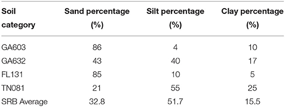
Table 1. The characteristics of alteration of soil texture.
The third factor to be analyzed was the terrain slope. We examined the difference between the slopes of the southeastern CONUS (Class #1) and SRB, which are <10% and ~30%, respectively. Thus, we implemented an experiment where the terrain slope was reduced by 80%, by changing the digital elevation data that were inputs to the data pre-processor (Shen et al., 2014) of PAWS+CLM. 80% was chosen because after this treatment, the average slopes of the SRB basins were similar to those in the Coastal Plain region.
Besides single factor experiments, we also evaluated how multiple factors interacted to impact hydrologic fluxes. After implementing the numerical experiments, we recalculated the SSCS from each perturbed simulation. The total simulated water stored in the soil column and groundwater in the model was used as the water storage, while streamflow was extracted from the simulated daily outflow from each subbasin.
The effects of the ML hypotheses can be demonstrated solely by visualizing the results from the experiments. However, as an exploratory step, here we also propose a quantitative, data-centric Bayesian framework to integrate data and the results from the modeling experiments. Essentially, the machine learning provides the prior, and the numerical experiments compute a likelihood for a factor being the causal factor. The two probabilities can be integrated using Bayes' law.
Here, we define y as the observed patterns and F as the list of perturbations of the “process parameters”, i.e. physical factors whose effects can be represented by perturbing our PBM. In the present example, F can take one of three values in {“soil thickness,” “soil texture,” “slope”}. When F is equal to “soil thickness,” the setup of the PBM experiment is to increase soil thickness, while leaving soil texture and slope untouched. We can then identify the factors causing the differences in observed patterns between instances using Bayes' law:
where P(F) is the prior probability of the process parameters being the cause of the observed differences between instances, to be obtained from the pure data-driven analysis (more below), L(y|F) is the likelihood that, after making the process perturbations in F, the differences in patterns in y are observed, P(y) = ∫ L(y|F)P(F)dF is the marginalized probability, and P(F|y) is then the probability that, given the evidence with the model experiments, F is the causal factor for the observed differences. In the Bayesian analysis here, we only consider the top three individual factors as potential values for F, and do not consider parameter interactions.
More specifically for this case, we start from basins that are by default of SSCS class #2 and #3 in the SRB, and ask whether a change in one of the physical factors could turn them into class #1. Therefore, P(F) is the prior probability of each process perturbation, and was calculated as the frequency that F appears as the first level split in the RF model trained to predict the distance to the class center #1; L(y|F) is the likelihood function for the perturbed model to produce class #1 basins. This likelihood was assessed using a Gaussian Mixture Model (GMM), which is a generalization from K-means clustering. Instead of predicting one class membership, the GMM generates a fuzzy membership for all classes. Our GMM used the clustering results of FS17, including the clusters' centroids, clusters' covariances, and the fraction of data points belonging to each class (more details of the GMM are in Appendix A). The marginalized probability, P(y), was computed by integration.
The definitions of P(F), which uses model visit frequency, may seem unestablished. However, in the world-shocking event where AlphaGo defeated the Go world champion, the algorithm selected the most visited move during its Monte Carlo tree search as its actual action (Silver et al., 2016). Their choice, also reliant on model visit frequency, also seemed informal, but it performed marvelously well. Our choices were based on the current best tool we have given the overall objective of this paper.
In this section, we first show the limitations of CART analysis and ML in general, and present multiple competing hypotheses from ML. After demonstrating the performance of the PAWS+CLM model for the Susquehanna River basin, we show results from the perturbation experiments. Finally, we put those results in the exploratory Bayesian framework and examine its usefulness.
While soil thickness was the most frequent factor that can predict the SSCS difference between class #1 and class #3 basins (Figures 4A,B), we found that soil texture (Figures 4C,D display the result for sand percentage), and terrain slope (Figures 4E,F) are competing hypotheses. The CART experiments with 20 different random seeds showed that there is a 75% chance that RockDep was selected as the top-level split, followed by Sand and then Slope. From the RF modeling, RockDep, Sand, and Slope have 21%, 17%, and 2% chances to be selected as the top-level split, respectively, with the other remaining chances mostly taken by climatic variables. The performance of these alternative models are weaker than soil thickness, but the difference, especially between soil thickness and soil texture, was not big enough to warrant confident rejection. These competing hypotheses exist because terrain slope, soil texture, and depth to bedrock covary in space. As we go from Appalachia (Appalachian Plateau, Piedmont, Valley and Ridge) to the Coastal Plain, simultaneously the terrain flattens, the soil texture becomes more sandy, and the soil thickness increases substantially.
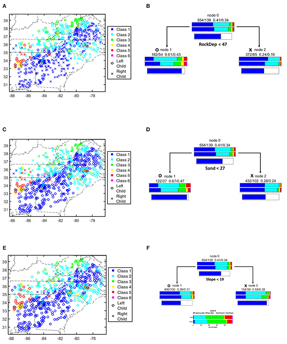
Figure 4. A one-level classification tree model picks up soil thickness (RockDep) as the main difference between two types of storage-stream flow correlation patterns compared to other physical factors like soil texture (result for sand percentage shown here, Sand) and terrain (Slope) (Reproduced from FS17 with permission). (A,C,E) Southeastern region of CONUS. Color indicates SSCS class, symbols indicate tree nodes for physical factor (RockDep, Sand, Slope). (B,D,F) One-level ad hoc trees to predict class #1 in (A,C,E) via physical factor (RockDep, Sand, Slope).
Besides random seeds, we also ran experiments with reduced training data points to examine the robustness of CART. We found that the frequency of the first-level criterion of the classification tree changed significantly when we randomly removed ~22% of the data. Moreover, in the extreme case, if we purposefully removed as few as 7 data points with the lowest sand percentages out of 693 total data points, the most important variable would change from “RockDep” to “Sand.”
These results all suggest that the CART analysis is not robust. CART is indeed problematic; however, this is not just an issue with CART, but more generically an issue with the statistical power of the data. It can be argued that there is not enough statistical power in the data to differentiate between the causal and the coincidental factors. Geoscientists are opportunistic in the sense that we can only examine basins with the combinations of land use, geology, soil texture, and slope that naturally exist in the world and have been, or are, under study. It is not be hard to imagine missing some critical combinations which would lead to erroneous conclusions.
More importantly, from these results, we extracted three factors that are treated as competing hypotheses that explains the main difference in SSCS between the Appalachian basins and their Southeast neighbors: soil thickness (RockDep), soil texture (Sand, Silt, or Clay), and terrain (Slope). Other basin parameters such as soil bulk density and land use have very low importance and can be ignored in later analysis. We then implemented changes in these factors in the process-based model to examine their impacts on the SSCS.
The daily observed USGS streamflow and simulated flow for a period of 18 years (2000–2017) were compared in Figure 5. The model had decent performance for streamflow simulation, especially within the baseflow and low flow periods (Figure 5), and captures the long-term streamflow pattern as well as some extreme high flows. The Nash-Sutcliffe model efficiency coefficient is not as high as in some of our previous applications (e.g., Shen and Phanikumar, 2010; Shen et al., 2014; Niu et al., 2017), due to the compromise in the 4 subbasins' parameter calibration. While the largest dam on the Susquehanna River, the Conowingo Dam, is downstream from our gage, there are other smaller dams in the basin that could have contributed to the mismatch. In addition, our experiences have indicated that NLDAS precipitation often underestimates the peak storms, leading to an under-estimation of peaks. As the main focus of the paper is not streamflow prediction, our calibration of the model is not extensive.
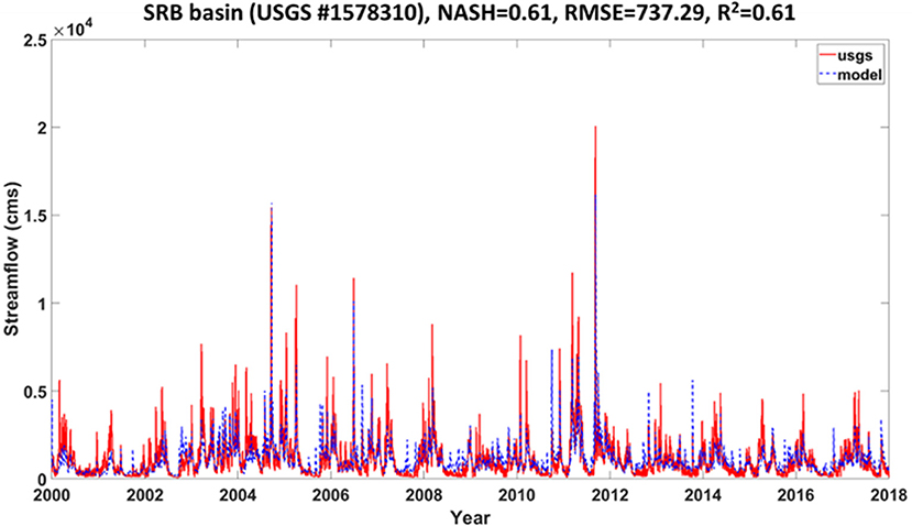
Figure 5. Model streamflow simulation of whole SRB streamflow simulation. The red solid line indicates the USGS measured streamflow, and the blue dashed line indicates the model's simulated flow.
It is easy to observe the impacts of soil thickness on the SSCS curves extracted from the default and perturbed simulations (Figure 6). On this figure, we colored experiments by whether they do have thicker soil implemented (adding 30 m to the soil thickness, shown in blue) or do not (shown in red). All four basins have similar patterns. The default SSCS (red x) curves are similar to SSCS classes #2 and #3 of FS17 (except the trough band of PIN, which is similar to Class #4), in that they have low correlations in peak-storage-low-flow bands, medium correlations in peak-storage-high-flow bands, and low correlations in trough-storage bands. These patterns all indicate a limited system memory; the water storage in the wet season has no impact on baseflow later in the water year. When we increased the soil thickness, the correlations in peak-storage-low-flow increased substantially, indicating that the annual-scale system memory had been enhanced. Except for the OCT subbasin, there is a clear separation between the red and blue points.
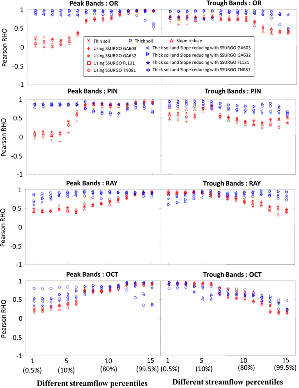
Figure 6. SSCS extracted from the numerical experiments. “Thin soil” is the default simulation with SRB-default parameters.
On the other hand, when soil texture was modified from the default (red x) into those from the Southeast (red plus, asterisk, square, and diamond), SSCS barely fluctuated, and results based on these southeastern soil textures were clustered closely with the default simulation. We could see that soil texture has a small impact: FL131 (red square) appears to encourage higher correlations across the spectrum as compared to the others. The notable soil texture characteristics were that GA603 had a high sand percentage (most were higher than 70%); GA632 had high sand and high silt percentages (summation of both were higher than 70%); FL131 was high in sand percentage (most were higher than 80%); and TN081 was high in silt percentage (most were higher than 50%). However, the magnitude of the impact of soil texture was not comparable to that of the soil thickness. According to the likelihood value calculated by the GMM, with all default parameters, OR belongs to Class #2 (highest probability, almost 1) and PIN belongs to Class #2 with a likelihood of 0.75 (Figures 7A,B). In contrast, all experiments with “thick soil” had SSCS class #1. Some parameter interaction can be observed, but its effects were minor compared to the impact of soil thickness.
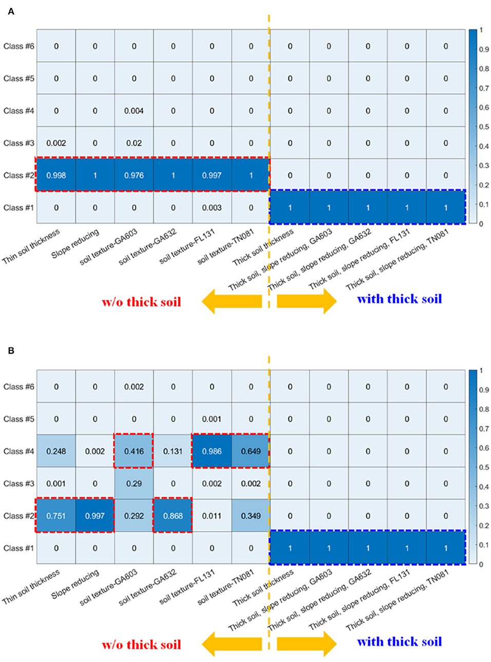
Figure 7. The likelihood function L(y|F) as calculated by GMM in different PAWS+CLM experiments. Deeper blue color highlights higher probability. Here, we only show the (A) OR and (B) PIN subbasins, but the other 2 subbasins have similar results (Appendix B).
From the experiments where we replaced forcing data in the SRB with those from the Coastal Plain region, we found the impacts of climate on SSCS classes (or GMM likelihoods) to be small (data not shown here). In fact, going from Appalachia in the North to the Coastal Plain in the South, we saw a lower fraction of precipitation as snow, which should have reduced storage-streamflow relationships, but this effect ran counter to the observation of higher correlations between storage and streamflow in the south. Apparently, the effects of climatic variables were not as strong as the physical basin parameters, and were also coincidental factors. Hence, they were not further examined.
According to the Bayesian inference framework in Equation 1, the soil thickness factor had the highest posterior probability (Table 2). Although soil texture also had a prior that was comparable to that of soil thickness, experiments that only perturbed soil had very low likelihood functions, lowering its posterior to almost zero. Terrain slope had a lower prior (although it was higher than other physical factors which were examined but not mentioned here), and its likelihood was also low, indicating that it was only a coincidental factor, not causal.
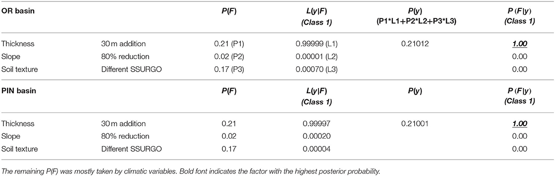
Table 2. Calculations of the data-centric Bayesian inference framework for three factors.
These results unequivocally support soil thickness as the causal factor of SSCS differences between Appalachian basins and those on the southeastern Coastal Plain, whereas soil texture and slope were merely coincidental factors. It is notable that the PBM was needed to break the practical tie between the priors of soil texture and soil thickness. From these results, we can conclude that in general, systems with large soil thickness have longer memory, allowing water from the recharge season to accumulate, which thus impacts the baseflow in the hot summers. Although more sandy soil could allow for more infiltration and hence mildly boost storage-streamflow correlations, its impact was apparently not comparable to that of soil thickness. This contrast was automatically highlighted by the Bayesian framework proposed here.
In this case study, ML allowed us to focus on only three factors prior to running any numerical experiments. If we were to run the hydrologic model to assess all of the 11 factors analyzed in CART, assuming 3 levels for each factor, 311 model runs would be needed, but in this analysis we only ran 11 jobs. Not only does this provide savings of computational power and time, but also means that we need to objectively confront our PBMs with the identified ML hypotheses. If the PBM at hand is not able to represent the effects of these factors, one needs to take note and either refine the PBM or select a different one. Because of the target, inputs, training data, and other aspects of ML still needing to be defined by humans, it is not unbiased, and fairness in artificial intelligence is a big topic (Zou and Schiebinger, 2018). However, as long as the initial ML problem is posed inclusively, ML can be relatively impartial compared to only using one PBM and starting only from expert-conceived hypotheses. The PBM was also critically important here, allowing us to study causal relationships and nuances of parameter interactions, where data may not be sufficient for complete analysis via ML.
The proposed framework is very different from that of physics-guided machine learning (PGML) (Ganguly et al., 2014; Jia et al., 2019) in that it utilizes established PBMs, which are valuable assets which the geoscience community has accumulated over the past decades, as the backbone of the analysis, whereas PGML relies on ML algorithms as the backbone. While one can easily encode simple principles such as mass and energy conservation in the loss function for PGML, it will be quite difficult to similarly express the complex physical processes and cross-domain interactions encoded in complex PBMs. Another PGML method is to pre-train a ML network with outputs from the PBM; in the future it will certainly be interesting to compare these methods in terms of their capability and clarity of finding explanations.
The proposed data-centric Bayesian framework is raised here for the first time, and is thus only exploratory. It requires the definition of a prior (from ML), a proper PBM, a likelihood function (calculated by the GMM), and a marginalization strategy. Upon proper definition of the prior and likelihood functions, this framework can be autonomously executed. The prior is obtained purely from data analysis of GRACE and streamflow data while the posterior mostly depends on the assumed model dynamics which were built from physical laws such as the Richards equation, diffusive flow equations, and ecosystem equations. Each one of these choices can have alternatives, and may involve arbitrary decisions that lead to debates. We fully recognize that the choices we made could be improved in the future. However, our goal here was to highlight the value of both PBM and ML, and to inspire exploration into the diverse ways that both approaches can be coupled together for the advancement of knowledge.
Here we used an interpretable machine learning method (classification tree) for illustrative purposes, essentially to obtain a parameter importance ranking and an estimate of a prior. Other methods such as linear regression, support vector machines, or deep learning neural networks could also be used to provide the prior. Time series deep learning-based models (Fang et al., 2017, 2018; Fang and Shen, 2020; Feng et al., 2020), have also emerged and are transforming hydrology (Shen, 2018), but they are less interpretable. The main purpose of the ML algorithm is to obtain a parameter importance ranking and an estimate of prior. Besides algorithm-specific methods such as layer-wise relevance propagation (Bach et al., 2015), many model-agnostic methods, e.g. permutation feature importance (Fisher et al., 2019) or forward/backward feature selection, exist to obtain parameter importance rankings and priors. On the other hand, interpretability is not necessarily required if the purpose is to autonomously discover knowledge, e.g., if the purpose is for an AI agent to reduce uncertainty in the framework of active learning (Settles, 2012). The only true requirements are that the hypothesis generated by the ML algorithm can be translated into a PBM configuration and used to make perturbations, and that the likelihood of those configurations can be evaluated.
Here we have proposed a Bayesian framework that combines machine learning and process-based modeling to overcome limitations of both approaches. In this framework, machine learning is first used to generate competing hypotheses that are consistent with existing data. These hypotheses are subsequently implemented as perturbed process-based model simulations, which help to distinguish between causal and coincidental factors. This framework can be executed by a program and could be regarded as giving PBMs to machine learning as diagnosis tools. ML has its limitations regarding robustness, the statistical power of limited data, and causal reasoning, but it allows us to rapidly focus on several competing hypotheses and limit our subjective bias when choosing a model.
We tested the framework using the example of inferring the physical factor that controls storage-streamflow correlation behaviors across the gradients from Appalachia to the Coastal Plain. Although machine learning suggested that soil thickness and soil texture have similar prior probabilities of being the causal factor, the PBM experiments unequivocally supported soil thickness. This example highlights the value of the PBM in the era of big data, and promotes an alternative ML-PBM integration methodology to physics-guided machine learning, as it works with complicated, established PBMs.
The details of the Gaussian Mixture model and a map of physiographic provinces are available in Supplemental Materials. Streamflow data can be downloaded from the U.S. Geological Survey Water Data for the Nation website (http://dx.doi.org/10.5066/F7P55KJN). GRACE TWSA data can be downloaded from GRACE monthly mass grids (https://grace.jpl.nasa.gov/data/get-data/). CART, RF, and GMM codes can be downloaded from Scikit-learn (https://scikit-learn.org/stable/). Our CART code and the PAWS-CLM code are available at doi: 10.5281/zenodo.4019836. The input to one of the subbasins is available at http://water.engr.psu.edu/shen/Data/PIN.zip.
CS conceived the study. WP-T ran the experiments, prepared the visualization, and wrote the initial draft. KF and XJ assisted with the experiments. CS and KL edited the manuscript.
This work was supported by the Office of Biological and Environmental Research of the U.S. Department of Energy under contract DE-SC0016605.
The authors declare that the research was conducted in the absence of any commercial or financial relationships that could be construed as a potential conflict of interest.
The Supplementary Material for this article can be found online at: https://www.frontiersin.org/articles/10.3389/frwa.2020.583000/full#supplementary-material
Bach, S., Binder, A., Montavon, G., Klauschen, F., Müller, K.-R., and Samek, W. (2015). On pixel-wise explanations for non-linear classifier decisions by layer-wise relevance propagation. PLoS ONE 10:e0130140. doi: 10.1371/journal.pone.0130140
Beven, K., and Binley, A. (1992). The future of distributed models: model calibration and uncertainty prediction. Hydrol. Process. 6, 279–298. doi: 10.1002/hyp.3360060305
Breiman, L., Friedman, J., Olshen, R., and Stone, C. J. (1984). Classification and Regression Trees. Boca Raton, FL: CRC Press.
Collins, W. D., Bitz, C. M., Blackmon, M. L., Bonan, G. B., Bretherton, C. S., Carton, J. A., et al. (2006). The community climate system model version 3 (CCSM3). J. Clim. 19, 2122–2143. doi: 10.1175/JCLI3761.1
Dickinson, R. E., Oleson, K. W., Bonan, G., Hoffman, F., Thornton, P., Vertenstein, M., et al. (2006). The community land model and its climate statistics as a component of the community climate system model. J. Clim. 19, 2302–2324. doi: 10.1175/JCLI3742.1
Fang, K., Ji, X., Shen, C., Ludwig, N., Godfrey, P., Mahjabin, T., et al. (2019). Combining a land surface model with groundwater model calibration to assess the impacts of groundwater pumping in a mountainous desert basin. Adv. Water Resourc. 130, 12–28. doi: 10.1016/j.advwatres.2019.05.008
Fang, K., Pan, M., and Shen, C. (2018). The value of SMAP for long-term soil moisture estimation with the help of deep learning. IEEE Trans. Geosci. Remote Sens. 57, 2221–2233. doi: 10.1109/TGRS.2018.2872131
Fang, K., and Shen, C. (2017). Full-flow-regime storage-streamflow correlation patterns provide insights into hydrologic functioning over the continental US. Water Resourc. Res. 53, 8064–8083. doi: 10.1002/2016WR020283
Fang, K., and Shen, C. (2020). Near-real-time forecast of satellite-based soil moisture using long short-term memory with an adaptive data integration kernel. J. Hydrometeorol. 21, 399–413. doi: 10.1175/JHM-D-19-0169.1
Fang, K., Shen, C., Kifer, D., and Yang, X. (2017). Prolongation of SMAP to spatio-temporally seamless coverage of continental US using a deep learning neural network. Geophys. Res. Lett. 44, 11030–11039. doi: 10.1002/2017GL075619
Feng, D., Fang, K., and Shen, C. (2020). Enhancing streamflow forecast and extracting insights using long-short term memory networks with data integration at continental scales. Water Resourc. Res.56:e2019WR026793. doi: 10.1029/2019WR026793
Fisher, A., Rudin, C., and Dominici, F. (2019). All models are wrong, but many are useful: Learning a variable's importance by studying an entire class of prediction models simultaneously. J. Mach. Learn. Res. 20, 1–81. Available online at: https://jmlr.org/papers/v20/18-760.html
Ganguly, A. R., Kodra, E. A., Agrawal, A., Banerjee, A., Boriah, S., Chatterjee, S. N., et al. (2014). Toward enhanced understanding and projections of climate extremes using physics-guided data mining techniques. Nonlinear Process. Geophys. 21, 777–795. doi: 10.5194/npg-21-777-2014
Guber, A. K., Pachepsky, Y. A., Th van Genuchten, M., Simunek, J., Jacques, D., Nemes, A., et al. (2009). Multimodel simulation of water flow in a field soil using pedotransfer functions. Vadose Zone J. 8, 1–10. doi: 10.2136/vzj2007.0144
Ho, T. K. (1995). “Random decision forests,” in Proceeding ICDAR '95 Proceedings of the Third International Conference on Document Analysis and Recognition (Montreal, QC: IEEE).
Ji, X., Lesack, L., Melack, J. M., Wang, S., Riley, W. J., and Shen, C. (2019). Seasonal and inter-annual patterns and controls of hydrological fluxes in an Amazon floodplain lake with a surface-subsurface processes model. Water Resourc. Res. 55, 3056–3075. doi: 10.1029/2018WR023897
Ji, X., and Shen, C. (2018). The introspective may achieve more: enhancing existing geoscientific models with native-language structural reflection. Comput. Geosci. 110, 32–40. doi: 10.1016/j.cageo.2017.09.014
Ji, X., Shen, C., and Riley, W. J. (2015). Temporal evolution of soil moisture statistical fractal and controls by soil texture and regional groundwater flow. Adv. Water Resourc. 86, 155–169. doi: 10.1016/j.advwatres.2015.09.027
Jia, X., Karpatne, A., Willard, J., Steinbach, M., Read, J., Hanson, P. C., et al. (2018). “Physics guided recurrent neural networks for modeling dynamical systems: application to monitoring water temperature and quality in Lakes,” in 8th International Workshop on Climate Informatics.
Jia, X., Willard, J., Karpatne, A., Read, J., Zwart, J., Steinbach, M., et al. (2019). “Physics guided RNNs for modeling dynamical systems: a case study in simulating lake temperature profiles,” in Proceedings of the 2019 SIAM International Conference on Data Mining (Calgary: Society for Industrial and Applied Mathematics Publications), 558–566. doi: 10.1137/1.9781611975673.63
Karpatne, A., Atluri, G., Faghmous, J. H., Steinbach, M., Banerjee, A., Ganguly, A., et al. (2017). Theory-guided data science: a new paradigm for scientific discovery from data. IEEE Trans. Knowl. Data Eng. 29, 2318–2331. doi: 10.1109/TKDE.2017.2720168
Kavetski, D., Kuczera, G., and Franks, S. W. (2006). Bayesian analysis of input uncertainty in hydrological modeling: 2. Application. Water Resourc. Res. 42. doi: 10.1029/2005WR004376
Lawrence, D. M., Oleson, K. W., Flanner, M. G., Thornton, P. E., Swenson, S. C., Lawrence, P. J., et al. (2011). Parameterization improvements and functional and structural advances in version 4 of the community land model. J. Adv. Model. Earth Syst. 3. doi: 10.1029/2011MS00045
Maxwell, R. M., and Condon, L. E. (2016). Connections between groundwater flow and transpiration partitioning. Science 353, 377–380. doi: 10.1126/science.aaf7891
May, J. (2011). On Ancient Susquehanna River, Flooding's a Frequent Fact. Associated Press. Available online at: http://cumberlink.com/news/local/on-ancient-susquehanna-river-flooding-s-a-frequent-fact/article_ee769266-db2f-11e0-945d-001cc4c002e0.html (accessed November 01, 2020).
Mitchell, K. E. (2004). The multi-institution North American land data assimilation system (NLDAS): utilizing multiple GCIP products and partners in a continental distributed hydrological modeling system. J. Geophys. Res. 109:D07S90. doi: 10.1029/2003JD003823
Nash, J. E., and Sutcliffe, J. V. (1970). River flow forecasting through conceptual models part I — a discussion of principles. J. Hydrol. 10, 282–290. doi: 10.1016/0022-1694(70)90255-6
Nearing, G. S., Mocko, D. M., Peters-Lidard, C. D., Kumar, S. V., and Xia, Y. (2016). Benchmarking NLDAS-2 soil moisture and evapotranspiration to separate uncertainty contributions. J. Hydrometeorol. 17, 745–759. doi: 10.1175/JHM-D-15-0063.1
Niu, J., Shen, C., Chambers, J., Melack, J. M., and Riley, W. J. (2017). Interannual variation in hydrologic budgets in an Amazonian watershed with a coupled subsurface—land surface process model. J. Hydrometeorol. 18, 2597–2617. doi: 10.1175/JHM-D-17-0108.1
NRCS (2010). SSURGO Soil Survey Geographic Database. Natural Resources Conservation Service; Natural Resources Conservation Service, United States Department of Agriculture. Available online at: https://data.nal.usda.gov/dataset/soil-survey-geographic-database-ssurgo (accessed November 01, 2020).
Oleson, K., Lawrence, D. M., Bonan, G. B., Flanner, M., Kluzek, E., Lawrence, P., et al. (2010). Technical Description of version 4.0 of the Community Land Model (CLM). Boulder, CO: NCAR Technical Note, NCAR/TN-478+STR.
Pelletier, J. D., Broxton, P. D., Hazenberg, P., Zeng, X., Troch, P. A., Niu, G.-Y., et al. (2016). A gridded global data set of soil, intact regolith, and sedimentary deposit thicknesses for regional and global land surface modeling. J. Adv. Model. Earth Syst. 8, 41–65. doi: 10.1002/2015MS000526
Poff, N. L., and Allan, J. D. (1995). Functional organization of stream fish assemblages in relation to hydrological variability. Ecology 76, 606–627. doi: 10.2307/1941217
Raje, D., and Krishnan, R. (2012). Bayesian parameter uncertainty modeling in a macroscale hydrologic model and its impact on Indian river basin hydrology under climate change. Water Resourc. Res. 48. doi: 10.1029/2011WR011123
Read, J. S., Jia, X., Willard, J., Appling, A. P., Zwart, J. A., Oliver, S. K., et al. (2019). Process-guided deep learning predictions of lake water temperature. Water Resourc. Res. 55, 9173–9190. doi: 10.1029/2019WR024922
Reager, J. T., Thomas, A., Sproles, E., Rodell, M., Beaudoing, H., Li, B., et al. (2015). Assimilation of GRACE terrestrial water storage observations into a land surface model for the assessment of regional flood potential. Remote Sens. 7, 14663–14679. doi: 10.3390/rs71114663
Reager, J. T., Thomas, B. F., and Famiglietti, J. S. (2014). River basin flood potential inferred using GRACE gravity observations at several months lead time. Nat. Geosci. 7, 588–592. doi: 10.1038/ngeo2203
Russell, S., and Norvig, P. (2009). Artificial Intelligence: A Modern Approach 3rd Edn. Upper Saddle River, NJ: Prentice Hall.
Schaap, M. G., Leij, F. J., and Th van Genuchten, M. (2001). Rosetta: a computer program for estimating soil hydraulic parameters with hierarchical pedotransfer functions. J. Hydrol. 251, 163–176. doi: 10.1016/S0022-1694(01)00466-8
Settles, B. (2012). “Active learning,” in Synthesis Lectures on Artificial Intelligence and Machine Learning, eds R. J. Brachman, W. W. Cohen, and T. G. Dietterich (Williston, VT: Norgan and Claypool), 1–114. doi: 10.2200/S00429ED1V01Y201207AIM018
Shen, C. (2018). A trans-disciplinary review of deep learning research and its relevance for water resources scientists. Water Resourc. Res. 54, 8558–8593. doi: 10.1029/2018WR022643
Shen, C., Laloy, E., Elshorbagy, A., Albert, A., Bales, J., Chang, F.-J., et al. (2018). HESS opinions: incubating deep-learning-powered hydrologic science advances as a community. Hydrol. Earth Syst. Sci. 22, 5639–5656. doi: 10.5194/hess-22-5639-2018
Shen, C., Niu, J., and Fang, K. (2014). Quantifying the effects of data integration algorithms on the outcomes of a subsurface–land surface processes model. Environ. Model. Softw. 59, 146–161. doi: 10.1016/j.envsoft.2014.05.006
Shen, C., Niu, J., and Phanikumar, M. S. (2013). Evaluating controls on coupled hydrologic and vegetation dynamics in a humid continental climate watershed using a subsurface—land surface processes model. Water Resourc. Res. 49, 2552–2572. doi: 10.1002/wrcr.20189
Shen, C., and Phanikumar, M. S. (2010). A process-based, distributed hydrologic model based on a large-scale method for surface–subsurface coupling. Adv. Water Resourc. 33, 1524–1541. doi: 10.1016/j.advwatres.2010.09.002
Shen, C., Riley, W. J., Smithgall, K. M., Melack, J. M., and Fang, K. (2016). The fan of influence of streams and channel feedbacks to simulated land surface water and carbon dynamics. Water Resourc. Res. 52, 880–902. doi: 10.1002/2015WR018086
Silver, D., Huang, A., Maddison, C. J., Guez, A., Sifre, L., van den Driessche, G., et al. (2016). Mastering the game of Go with deep neural networks and tree search. Nature 529, 484–489. doi: 10.1038/nature16961
Thomas, B. F., Vogel, R. M., Kroll, C. N., and Famiglietti, J. S. (2013). Estimation of the base flow recession constant under human interference. Water Resourc. Res. 49, 7366–7379. doi: 10.1002/wrcr.20532
Verhougstraete, M. P., Martin, S. L., Kendall, A. D., Hyndman, D. W., and Rose, J. B. (2015). Linking fecal bacteria in rivers to landscape, geochemical, and hydrologic factors and sources at the basin scale. Proc. Natl. Acad. Sci. U.S.A. 112, 10419–10424. doi: 10.1073/pnas.1415836112
Viglione, A., Merz, R., Salinas, J. L., and Blöschl, G. (2013). Flood frequency hydrology: 3. A bayesian analysis. Water Resourc. Res. 49, 675–692. doi: 10.1029/2011WR010782
Vrugt, J. A., Gupta, H. V., Bastidas, L. A., Bouten, W., and Sorooshian, S. (2003). Effective and efficient algorithm for multiobjective optimization of hydrologic models. Water Resourc. Res. 39. doi: 10.1029/2002WR001746
Vrugt, J. A., ter Braak, C. J. F., Diks, C. G. H., Robinson, B. A., Hyman, J. M., and Higdon, D. (2009). Accelerating markov chain monte carlo simulation by differential evolution with self-adaptive randomized subspace sampling. Int. J. Nonlinear Sci. Numerical Simul. 10, 273–290. doi: 10.1515/IJNSNS.2009.10.3.273
Yang, X., Barajas-Solano, D., Tartakovsky, G., and Tartakovsky, A. M. (2019). Physics-informed CoKriging: a gaussian-process-regression-based multifidelity method for data-model convergence. J. Comput. Phys. 395, 410–431. doi: 10.1016/j.jcp.2019.06.041
Yarnal, B., Johnson, D. L., Frakes, B. J., Bowles, G. I., and Pascale, P. (1997). The flood of '96 and its socioeconomic impacts in the susquehanna river basin. J. Am. Water Resourc. Assoc. 33, 1299–1312. doi: 10.1111/j.1752-1688.1997.tb03554.x
Keywords: Machine Learning (ML), process-based model (PBM), streamflow-storage relationships, data-centric, Bayes law, classification tree, soil texture
Citation: Tsai W-P, Fang K, Ji X, Lawson K and Shen C (2020) Revealing Causal Controls of Storage-Streamflow Relationships With a Data-Centric Bayesian Framework Combining Machine Learning and Process-Based Modeling. Front. Water 2:583000. doi: 10.3389/frwa.2020.583000
Received: 13 July 2020; Accepted: 30 September 2020;
Published: 27 November 2020.
Edited by:
Bhavna Arora, Lawrence Berkeley National Laboratory, United StatesReviewed by:
Jeffrey Michael Sadler, United States Geological Survey (USGS), United StatesCopyright © 2020 Tsai, Fang, Ji, Lawson and Shen. This is an open-access article distributed under the terms of the Creative Commons Attribution License (CC BY). The use, distribution or reproduction in other forums is permitted, provided the original author(s) and the copyright owner(s) are credited and that the original publication in this journal is cited, in accordance with accepted academic practice. No use, distribution or reproduction is permitted which does not comply with these terms.
*Correspondence: Chaopeng Shen, Y3NoZW5AZW5nci5wc3UuZWR1
Disclaimer: All claims expressed in this article are solely those of the authors and do not necessarily represent those of their affiliated organizations, or those of the publisher, the editors and the reviewers. Any product that may be evaluated in this article or claim that may be made by its manufacturer is not guaranteed or endorsed by the publisher.
Research integrity at Frontiers
Learn more about the work of our research integrity team to safeguard the quality of each article we publish.