 Henning Oppel
 Benjamin Mewes
- 1Center for Environmental System Research, Kassel University, Kassel, Germany
- 2Institute of Hydrologic Engineering and Water Management, Ruhr-University Bochum, Bochum, Germany
Can machine learning effectively lower the effort necessary to extract important information from raw data for hydrological research questions? On the example of a typical water-management task, the extraction of direct runoff flood events from continuous hydrographs, we demonstrate how machine learning can be used to automate the application of expert knowledge to big data sets and extract the relevant information. In particular, we tested seven different algorithms to detect event beginning and end solely from a given excerpt from the continuous hydrograph. First, the number of required data points within the excerpts as well as the amount of training data has been determined. In a local application, we were able to show that all applied Machine learning algorithms were capable to reproduce manually defined event boundaries. Automatically delineated events were afflicted with a relative duration error of 20 and 5% event volume. Moreover, we could show that hydrograph separation patterns could easily be learned by the algorithms and are regionally and trans-regionally transferable without significant performance loss. Hence, the training data sets can be very small and trained algorithms can be applied to new catchments lacking training data. The results showed the great potential of machine learning to extract relevant information efficiently and, hence, lower the effort for data preprocessing for water management studies. Moreover, the transferability of trained algorithms to other catchments is a clear advantage to common methods.
1. Introduction
Machine-learning has proven its capability in a vast range of applications, especially in those cases when a certain pattern has to be revealed from a huge data archive in order to reproduce it afterwards. Water management tasks require these capabilities in various steps. Natural and anthropocentric processes have to be reproduced in order to model future events and behaviors (Mount et al., 2016). Hence, machine learning (ML) has been applied in a broad range of applications, like streamflow simulation (Shortridge et al., 2016), the interpretation of remote sensing images (Mountrakis et al., 2011), modeling of evapotranspiration (Tabari et al., 2012), rainfall forecasting (Yu et al., 2017), process analysis (Oppel and Schumann, 2020), and many more. However, all water related tasks require pre-processed data. Pre-processing is in this case defined as the extraction of the relevant information from raw data. A typical example is the need for direct runoff flood events that have to be extracted from continuous time series of discharge. This kind of information can be used for flood event research, training of hydrological models for flood forecasting, design tasks, etc. Despite its relevance and expense, there is no single accepted method to efficiently automate this problem.
Especially the separation of rain fed direct runoff from the base flow, i.e., discharge from deeper soil layers and groundwater with higher transit times, has been subject to much scientific work. This might be due to the fact that rain fed direct runoff events are especially relevant for flood security (Fischer, 2018). The most accurate way to separate direct and base flow runoff in order to define flood events is to use tracer based methods (Klaus and McDonnell, 2013; Weiler et al., 2017). However, tracer data are only rarely available and are not collected on a continual basis. Hence, their application is limited to very few case studies and is not suitable for automated information extraction especially for long time series.
There are three main groups of methods to extract flood events from continuous time series: graphical methods, digital filtering and recession based methods. Graphical approaches (Hall, 1968; Maidment, 1993) are well-established in the water management community, yet they rely on assumptions and experience of the user (Mei and Anagnostou, 2015). Moreover, these types of methods cannot be applied to large data sets and do not allow for automation. Digital filtering techniques overcame this drawback. These methods use a one- (Lyne and Hollick, 1979), two- (Su, 1995; Eckhardt, 2005) or three-parametric (Eckhardt, 2005) base equation to reproduce the long wave response of a hydrograph. The calculated response is treated as the baseflow, the residual of baseflow and hydrograph is treated as the direct runoff. The intersections of baseflow and direct runoff curves can be treated as beginning and end of individual events. These methods are especially applicable to extract information from long time series and allow for automation, like Merz et al. (2006), Merz and Blöschl (2009), and Su (1995). Gonzales et al. (2009) and Zhang et al. (2017) stated that digital filtering techniques, especially the three-parametric filter (Eckhardt, 2005), delivers superior results to all other methods. However, they also pointed out that these methods require local calibration.
The calibration process limits the application of a digital filter to its fitted catchment. Moreover, the missing physical reasoning of the parameters introduced parameter uncertainty to the process (Furey and Gupta, 2001; Blume et al., 2007; Stewart, 2015). Recession based methods try to overcome the lack of physical reasoning (Tallaksen, 1995; Hammond and Han, 2006; Mei and Anagnostou, 2015; Dahak and Boutaghane, 2019). They either rely on a linear (Blume et al., 2007) or non-linear (Wittenberg and Aksoy, 2010) connection between storage and the active process that defines the hydrograph. Other methods try to estimate the parameters of digital filter from the recession curves (Collischonn and Fan, 2012; Mei and Anagnostou, 2015; Stewart, 2015). The drawback of these approaches is the missing automation. Stewart (2015) analyzed several recession curves and their connections to the separation of direct runoff and base flow. Although a connection between direct runoff and base flow was identified, they also found that recession analysis relying on streamflow data solely can be misleading. Under different conditions of the catchment different processes are active, and hence, the connection between storage and runoff changes. Beside this process uncertainty most methods require calibration just like digital filtering techniques and cannot be transferred to other basins.
As already pointed out, the common methods either lack a way to automate them or they require local calibration. Either way, the effort to extract the relevant information is high. Another drawback is that especially the physically based methods search for the true separation of direct runoff and base flow. But, in some cases this might not be the target of a separation. For example: if the task is to evaluate just the first peak of each flood event, no common method can adopt to that target. The power of ML algorithms to detect patterns and to reproduce them in further application could be a solution to this topic. Thiesen et al. (2019) demonstrated that data-driven approaches with different predicors can be applied to the task of hydrograph separation. They found that models using discharge as predictors returned the best results. Although their automated flood event separation performed well, they required a large amount of training data which is limiting the applicability of their approach. Thiesen et al. (2019) estimated a label (flood event / no flood event) for each time step of the continuous time series and, hence, searched for the true separation of direct runoff and base flow. As stated before, this might not be applicable in all cases. Therefore we assumed that the event, i.e., the time stamp of the flood peak is known, but the time of event beginning and end are unknown.
In the first part of the study we assessed which part of a flood hydrograph is relevant to determine the begin and end of the event. Based on a training set generated by expert knowledge we analyzed how many points from a hydrograph excerpt are needed to estimate the event boundaries. Moreover, we analyzed which machine learning algorithms are suitable for this type of problem and how many training data is required to automate the separation process. A major shortcoming of common methods is the local bound applicability. Therefore, we tested if trained algorithms could successfully be applied in new catchments on a regional and trans-regional scale.
2. Materials and Methods
In this section we will shortly introduce the case study basins of the Upper Main and the Regen. In the subsequent section, the ML algorithms and their settings will be presented. This section is completed with the introduction of the entropy concept and the performance criteria used to evaluate the ML-algorithms.
2.1. Data
For this study, continuous time series from 15 gauges in south-east Germany have been used. Five gauges from the basin of the Upper Main have been used for local application and the tests on required training data and predictors. Additional five gauges from the Upper Main basin and five other gauges from the Regen basin have been used for regional and trans-regional validation of the trained algorithms solely. The time series had an hourly temporal resolution and covered the time span from 2001 to 2007 in the Upper Main basin, 1999 to 2012 in the Regen basin.
We assumed that users know what kind of flood events they are interested in and just needs to automate the process of separation (Moreover, the process of peak identification can be automated with a peak-over-threshold (POT) method). Hence, we defined the time stamps of five highest discharge peaks per year as the events of interest. The number of five events per year has been chosen to create a large data basis while maintaining the focus on floods. To create a training and validation data set beginning tB and end tE of each event have been defined manually. Due to the focus on flood events our strategy for manual flood separation was to capture begin and end of direct runoff. Although precipitation data was available, we excluded it on purpose to focus on the hydrographs. The begin of the direct runoff tB was defined as the first significant increase of discharge prior to the peak. The end of direct runoff tE was defined as either the last change of slope of the recession curve starting from the peak before the next rise, or the last ordinate of the recession curve before the next event (compare Figure 1). Target variables tB and tE were defined as difference between the time stamp of the peak and the time stamp of the events begin/end.
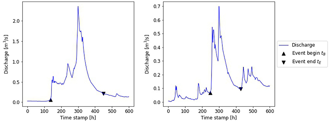
Figure 1. Flood events observed at gauge Friedersdorf with manual defined markers of event begin tB and end tE to capture direct runoff.
As the spatial arrangement of the chosen gauges shows (Figure 2), training and validation gauges have been selected to cover similar relationships of neighboring and nested catchments. Additionally, the training and validation sets have been compiled to cover the same ranges of catchments area. Each set comprises small catchments with an area between 10 and 100 km2 and large catchments with an area between 100 and 1,400 km2 (compare Table 1).
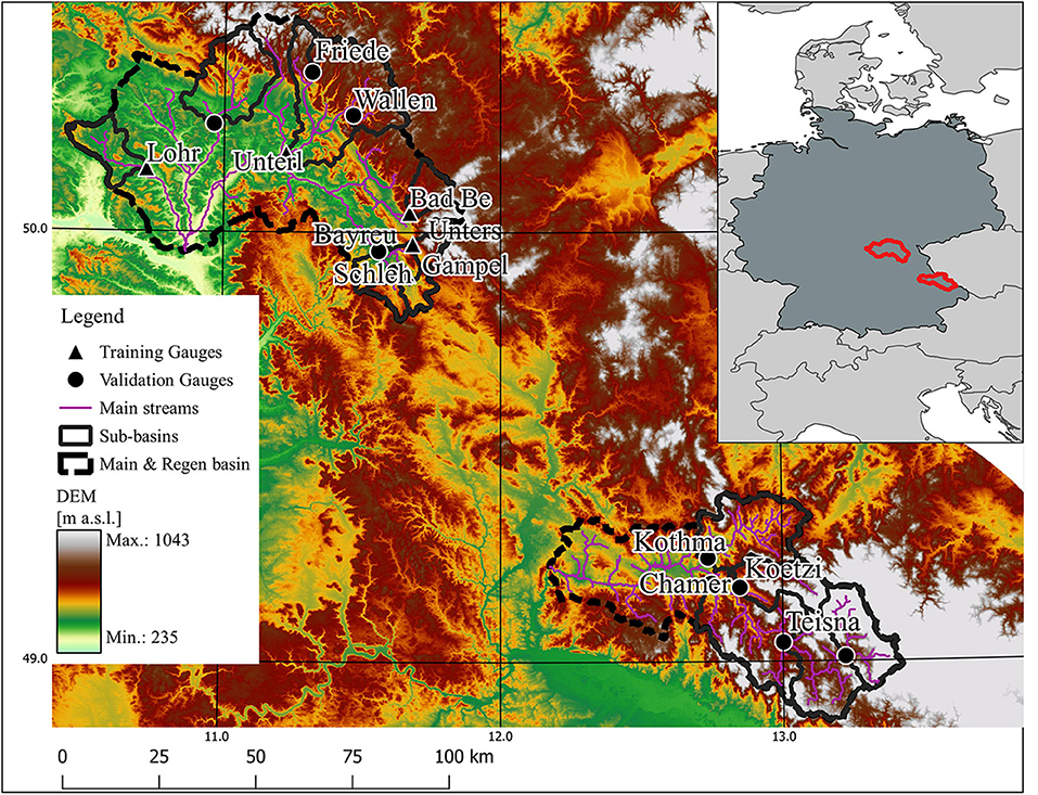
Figure 2. Case study basins of the Upper Main (upper left) and Regen (lower right) in south-east Germany. Five gauges (triangle) have been used for local application and as training data for (trans-) regional application (circle).
Table 1. Gauges and catchment areas in the case study regions.
The transferability of trained ML algorithms was analyzed by using a regional model strategy. The ML algorithms were trained with the data from the five gauges from the Training data set, defined in Table 1. All Training gauges were located in the upper Main basin. For validation the trained algorithms were used to estimate tB and tE for flood events observed at gauges from the regional and trans-regional data set (compare Table 1).
2.2. Machine Learning Algorithms
The No-free-Lunch-Theorem pays its tribute to the plethora of available ML-algorithms and reduces the problem of choice to an optimization problem: If an algorithm performs well on a certain class of problems then it necessarily pays for that with degraded performance on the set of all remaining problems. A certain algorithm is more or less suitable for a specific problem (Wolpert and Macready, 1997). Accordingly, several approaches have to be taken into account in parallel. Additionally, Elshorbagy et al. (2010a,b) found that a single algorithm is not able to cover the whole range of hydrologic variability. Hence, they recommended to use an ensemble of algorithms for water related tasks. In order to assess which type of algorithm is suitable to the addressed task of this study we used seven different algorithms (provided by Pedregosa et al., 2011 as Python package scikit-learn), representing five different algorithm structures.
Artificial neuronal networks (ANN) are the most commonly applied ML algorithms which is also true for hydrological applications (Minns and Hall, 2005; Solomatine and Ostfeld, 2008). The structure of an ANN is inspired by the structure of the human brain (Goodfellow et al., 2016). Multiple input features are connected through multiple neurons on a variable number of hidden layers with the output of the network. The output neuron represents the target variable of the regression (or classification) task. The hidden layers of the ANN define the level of abstraction of the problem. The more layers, the more abstraction is given to the input features (Alpaydin, 2010). Because this study addressed the topic of pattern recognition in hydrographs with a, to this point, unknown degree of abstraction, ANNs with different numbers of hidden layers have been applied. Specifically, an ANN with a single and an ANN with two hidden layers have been applied. The number of neurons per layer has been adjusted during the training process. Both regressors were based on the multi-layer perceptron and used a stochastic gradient descent for optimization (Goodfellow et al., 2016). Additionally, an Extreme Learning Machine (ELM) was added to the group of used algorithms. The ELM is a special type of ANN (Guang-Bin Huang et al., 2004) that was designed for a faster learning process. In a classic ANN each connection between neurons is assigned with a weight that is updated in the optimization process. An ELM has fixed weights for the connection between hidden layer and the output neuron. Only the remaining connections are optimized during the training process. Due to this simplification, the ELM learns faster while regression outputs remain stable (Guang-Bin Huang et al., 2004).
The three types of neuronal networks are accompanied by 4 other algorithms. As a representative for the similarity-based algorithms the K-nearest-neighbor (KNN) algorithms has been applied (Kelleher et al., 2015). Here, no model in the common sense is trained. For regression, the KNN uses the predictors to define similarity between the elements of a new data set and the known cases of the training data. The output is then defined as the average of the k-nearest elements. In this study, k was defined iteratively during the training process within a range of [5;10]. Parameter values for k outside the specified range were tested, but rarely proved to be a better alternative. In order to accelerate the training of the KNN, the comparatively small parameter space was chosen. A Support Vector Machine (SVM) algorithm, an error-based approach, has also been used in this study. The SVM fits a M-dimensional regression model to the given problem, where M can be greater than the dimension of the original feature space. To maintain a reasonable computation time, the SVM focuses on data points outside a certain margin around the regression line, the so-called support vectors (Cortes and Vapnik, 1995). Another type of ML-algorithm included in this study was a Classification and Regression Tree (CART). Regression trees are built node per node with a successive reduction of regression error between the estimates and the true values. CART-regressors have been used as base estimators for a Random Forest (RF) that has been used additionally in this study. The RFs consisted of 1,000 regression trees, each trained with a randomly chosen subset of the given training data. The average of all regression results is returned as estimate of the RF. We applied the RF due to its common application in hydrological studies (Yu et al., 2017; Addor et al., 2018; Oppel and Schumann, 2020). Moreover, the use of an ensemble regressor accounts for the recommendations of Elshorbagy et al. (2010a). Details on implementation are provided by Pedregosa et al. (2011).
The applied algorithms face several inherent problems and advantages, so the right choice of a suiting algorithm depends on the available data and the problem to be solved. SVMs, for example, work perfectly if the margin of the separating vector is small. Thus, they tend to overfit if that is not the case in the data they are trained on. Moreover, the choice of the internal kernel is not trivial and has impact on the results and the training behavior. CART trees are very comprehensible models and quickly converging models, but tend to overfit, so the remaining degrees of freedom have to be considered for an interpretation of CART results. RF on the other hand reduce to vulnerability of overfitting, yet the build less comprehensible outcomes due to the large number of possible model trees. ANNs are robust against overfitting, but require more data to converge in complex situations than the other approaches. ELM inherits the advantages and problems of ANNs and SVM. KNN converge very quickly and are often a suitable method. Nevertheless, the general ability of KNN for ML prediction requires information on internal structure of the data and its internal clustering of groups.
2.3. Shannon Entropy
The entropy concept, introduced by Shannon (1948), is the underlying concept of information theory (Cover and Thomas, 2006). Shannon's entropy concept is used to determine the information content within a given data set. Entropy H is calculated for a discrete random variable X with possible values x1, …, xn by:
where P(xi) is the probability that X takes exactly the value xi. The basis b of the log-function can take any value, but is usually set to b = 2, which gives H the unit bit. As Equation (1) shows, the entropy value is a measure for uncertainty of the considered variable. If all samples drawn from X would take the same value, the probability of this value would be 1 and hence the entropy would be equal to 0.0, because one would be absolutely certain about the outcome of new samples drawn from X. The entropy increases to a value of 1.0 if the sample would be equally distributed on two outcomes (Kelleher et al., 2015). The higher the entropy, the wider the histogram of X is spread.
The problem with Equation (1) is that it can only be applied to discrete data. Unfortunately most hydrological relevant data is continuous. This was also the case in this study, because the ordinates of the hydrograph are intended to determine the events temporal boundaries. Gong et al. (2014) showed that the use of frequency histograms, which is also refereed as Bin Counting, is a feasible and reliable approach to represent the continuous as a discrete distribution function. To apply Bin Counting the width of bins has to be determined. Scott (1979) proposed the following estimator for the optimal bin-width h*:
where σ is the standard deviation of the data and N is the number of samples. We followed the recommendations of Scott (1979) and Gong et al. (2014) and used Bin Counting to calculate the entropy of the predictor and target variables.
2.4. Performance Criteria
Estimation errors manifest as differences between estimated and manually defined time stamps of event begin and end, resulting in different event metrics duration and volume. The deviations of these metrics were used to define the performance criteria. First, the mean volume reproduction MVR was defined as follows:
where N is the number of considered events and V is the estimated (Est) or manual defined (Man) event volume. The MVR is defined within [0;+inf] with an optimal value of 1. The second metric accounts for the duration of the event. For each event two sets of time stamps are available: set M containing all time stamps of the manually separated event, and D containing all time stamps of the estimated event. Time stamps within both sets are correctly ascertained time stamps by the ML-algorithm. This set I can be expressed as the intersection of both sets I = D∩M. Temporal coverage of an estimated event has been calculated as the ratio of the cardinalities of I and M, i.e., the ratio of correctly ascertained time stamps and the true number of event time stamps:
Temporal coverage COV is defined on [0;1] with an optimal value of 1. Note that COV only accounts for errors of time stamps, not the actual event duration. An estimate of event boundaries that sets event begin and end wrong, but outside of the true event boundaries, has a coverage equal to 1. However, the error will be accompanied by an MVR greater than one. The combined evaluation of COV and MVR reveals that the time stamps were set outside the true event boundaries.
3. Results
In this section, the analysis regarding the automation of the flood event hydrograph separation will be presented. Section 3.1 presents the selection of the ML-predictors, i.e., the number of hydrograph ordinates necessary to predict the event boundaries. This is followed by the results of the local application of the ML-algorithms (section 3.2).
3.1. Predictor Selection
As predictors for the estimation of event boundaries (time stamps of beginning and end of a flood event), we intended to use the ordinates of the hydrograph itself. Therefore, we had to determine the required amount of ordinates to achieve satisfactory results, while keeping the amount of predictors as low as possible to minimize the training effort of the ML-algorithms.
In other words we wanted to focus on the necessary hydrograph components to determine flood begin and end. In course of the graphical, manual separation (section 2.1) we observed that we mainly paid attention to the shape of the hydrograph in comparison to its closer hydrological context for our decisions. Transferring this to the numerical data of the hydrographs (Q) means that the set of hydrograph ordinate with the highest uncertainty about Q conveyed the highest amount of relevant information to the separation process. In order to determine the length of these sets we performed an entropy analysis for different lengths of sets (see below). We used the entropy metric to evaluate the information content H, because its values quantifies the uncertainty of a data set (compare section 2.3).
Although H calculated separately for the predictor and the target variable set allowed us to compare the information within the data, they do not tell us if these information coincide. The common approach to quantify the shared information content of data sets is to use the mutual information (MI) (Sharma and Mehrotra, 2014). The MI-value concept evaluates the joint probability distribution of two (or more) data sets and evaluates the information obtained from the predictor data set about the target data set. Due to the high dimension of our predictor data set (number of hydrograph ordinates between 10 and 600), the joint probability distributions could not be estimated. Hence, the concept of MI was not applicable. Hence, we relied on H calculated for target and predictor sets separately, to evaluate the predictor data sets. We assumed that an entropy value of the predictor set similar to the entropy of the target variable set is a necessary but not sufficient condition for an optimal predictor.
First, we calculated the entropy of the target variables for manually separated events, the time stamps of event beginning and end. Equation (1) and (2) were applied to all available data sets. We obtained average entropy values of HA = 1.55 bit for the event beginnings and HE = 2.15 bit for event ends. The standard deviation of HA and HE between the considered sub-basins was σ(HA) = 0.15 and σ(HE) = 0.39. The entropy values showed that the position of the flood beginning (in relation to the peak) is afflicted with less uncertainty than the end of the flood. A result that is in concordance with our experience from the manual flood separation.
In the second step of the analysis we calculated the entropy for different predictor data sets. The first data set evaluated consisted of 10 hydrograph ordinates, half of the ordinates prior to the peak the other half succeeded the peak. The amount of ordinates was increased incrementally up to 600 ordinates. The obtained entropy values showed that the data sets contained the highest entropy if only a few ordinates were used (Figure 3). Data sets with 10–50 ordinates, regardless of the sub-basin, showed an entropy value of H ≥ 3.7 bit which is equal to the sum of HA and HE. With an increasing amount of data the entropy values decreased significantly. With 500 data points considered, the entropy values lowered to a range of [2.0, 3.5] bit and did not change any further with increasing data points.
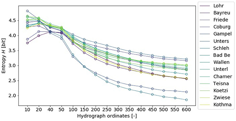
Figure 3. Entropy values of the data sets H considering a varying number of ordinates from hydrographs (number of ordinates considered on the abscissa).
In order to evaluate our assumption of the connection between equal entropy values and predictive performance, a test with different ML-algorithms in all sub-basins was carried out. Each data set was split randomly into training data (50%) and validation data (50%). Each ML-algorithm was trained and validated with the MVR (Equation 3) and COV (Equation 4). To minimize uncertainty due to the choice of training data, the evaluation was repeated 10-times for each data set. The obtained results were comparable in all applications. For the majority of catchments the best MVR-results (median and variance) were achieved with 40 or 50 ordinates used as predictors and the optimal COV with 50 ordinates. As an example the results of RF application in catchment Bad Berneck are shown in Figure 4 (Results for all other algorithms and catchments can be found in the Supplementary Material).
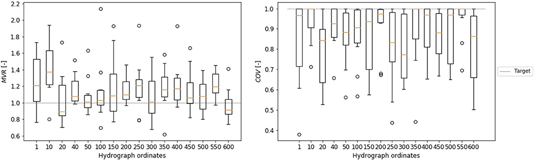
Figure 4. Dependence of the number of hydrograph ordinates and the mean volume reproduction (MVR) and temporal coverage (COV) of automatically separated flood events. Application of a trained RF in sub-basin Bad-Berneck.
Based on the experimental results and the evaluation of the entropy values we chose 40 ordinates, 20 prior to the peak and 20 succeeding the peak, as the predictor data set for the following analysis.
3.2. Automated Flood Hydrograph Separation
For each data set from the catchments marked as training gauges in Table 1 and Figure 2, we tested if flood hydrograph separation could be automated by means of ML. Like in the previous section, we randomly chose 50% of the available flood event data for training of the algorithms. Their performance was validated with withheld data from the respective gauge. Again, the procedure has been repeated to lower the uncertainty due to the randomly chosen subsets. In this case, 500 iterations were performed. For each event of the validation data, tB and tE were estimated with all available ML-algorithms (Figure 5).
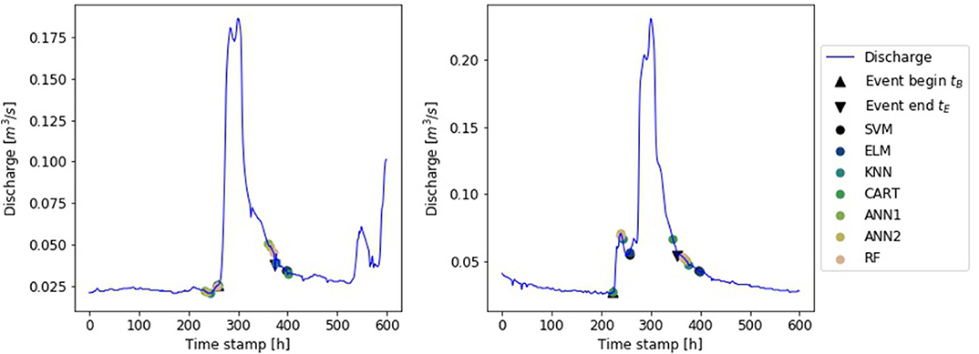
Figure 5. Hydrographs for two flood events at gauge Lohr with manually and automated defined markers of event begin tB and end tE.
The results showed that the ML-algorithms were able to perform the required automation task. However, they tended to overestimate the volume of the events (Figure 6), while the temporal coverage was met in the most cases (Figure 7). Only the ANN1 and ANN2 did not match the temporal extend of the events. The combination of a COV lower than 1 and MVR greater than 1 (compare Figure 5, right panel) showed that one time stamp was set too close to the peak, while the other was set too far from to peak. Giving a low coverage of the event and high volume error. In these cases it was the event start that was set too close to the peak and the end was set too far. A different behavior is visible in the results of the ELM and KNN. While the COV is close to 1, the MVR shows an average overestimation of event volume of 20%. This shows that ELM and KNN separated too long flood events. The best results were obtained with the RF and the SVM.
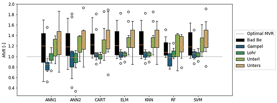
Figure 6. Mean volume reproduction (MVR) of the validation flood events in local application of trained artificial neuronal network with 1- (ANN1) and 2-hidden layers (ANN2), regression tree (CART), extreme learning machine (ELM), k-nearest-neighbor (KNN), random forest (RF), and support vector machine (SVM).
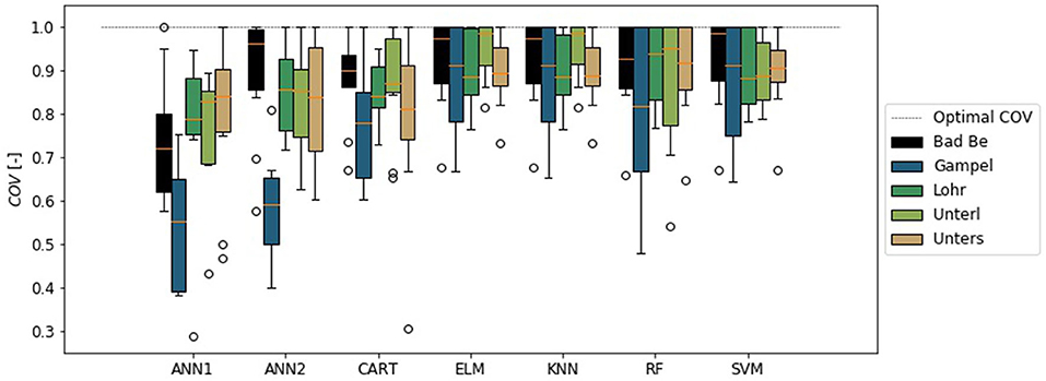
Figure 7. Temporal coverage (COV) of the validation flood event duration in local application of trained artificial neuronal network with 1- (ANN1) and 2-hidden layers (ANN2), regression tree (CART), extreme learning machine (ELM), k-nearest-neighbor (KNN), random forest (RF), and support vector machine (SVM).
The results also showed regional dependence of the model error. Independent from the chosen algorithm, Bad Berneck showed the highest volume errors, while Gampelmuehle showed the highest COV errors. It is striking that Gampelmuehle on the other hand showed one of the lowest volume errors, and Bad Berneck the lowest COV errors. Contrary to that, the three remaining basins showed comparable results for both criteria. An explanation for this observation lies within the response time of these catchments. In comparison to the other hydrographs, they are significantly more flashier and the duration of the flood events is significantly shorter.
4. Discussions
The presented results showed that ML is in general capable to automate the considered task. But several choices, like the amount of training data have to be discussed and the transferability of trained algorithms has to be tested. This sections provides discussions on these topics.
4.1. Training Data
The results showed that all algorithms could be used in local application to automate the task of flood event separation from continuous time series. Yet, the true benefit of the automation is unclear, because we randomly selected the size of the training data set. A true benefit for automation would be a minimal requirement of training data, because this would minimize the manual effort for separation. The results in section 3.2 showed that we could at least half the manual effort. But how many manually separated flood events are really necessary to train the algorithms?
To answer these questions, an iterative analysis has been performed. First, 25% of the available flood events were randomly chosen as validation data set and removed from the data pool. In the succeeding steps a variable amount of training data was chosen from this pool to train the ML-algorithms. In each step, the trained algorithms were validated with the same validation data set. In order to minimize uncertainty due to the randomly chosen data sets, this procedure was repeated 500 times.
The results showed that the required amount of training data was surprisingly low for all algorithms. The median MVR reached the optimum of MVR = 1.0 with the lowest amount of uncertainty with only 20–30% percent used training data (Figure 8, full plot with all ML-algorithms in the Supplementary Material). This was true for all ML-algorithms used in this study. The results for the COV criterion were similar to these findings. But in contrast to the MVR criterion, the uncertainty decreased slightly with increasing training data. The combined evaluation of MVR and COV showed different types of estimation errors. With a small data set the duration of the separated flood events is afflicted with higher uncertainty, while the true volume of the event is more likely to be met and vice versa for larger data sets. However, the orders of magnitude differ. The certainty of event duration does not increase to the same extent as the uncertainty of the volume increases.
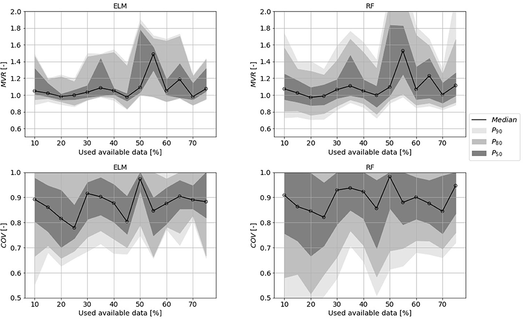
Figure 8. Dependence of mean volume reproduction (MVR)/temporal coverage (COV) and size of the training data set of a random forest (RF) and an extreme learning machine (ELM). Uncertainty belts drawn in gray scales for different probabilities (50, 80, 90%). The amount of training data has been raised incrementally to train the algorithms and were validated in each step with the same data set, containing 25% of the available data.
Note that in this study only 20 events per sub-basin were available, which means that a training data set of 4–5 manually separated flood events was a sufficient training data set for the automation of the task.
4.2. Transferability
In this section we present the results of the conducted test on the ability to transfer the trained algorithms to other catchments. First, a regional transfer has been tested. Here, we used the data sets from the local application (sections 3.2, 4.1) to train the ML-algorithms and validated their performance at five new gauges in the same basin, i.e., regional neighborhood (Figure 2). Likewise to the procedure in section 4.1, we analyzed the impact of training data on the performance. Here, we had a total of 117 flood events for training and validated with the individual data sets from the new five catchments.
The performance of the ANN1 and ANN2 stabilized at 30–40% of used data for both criteria (Figure 9). Estimates from both algorithms reached a median MVR≈1.05 and a median COV ≤ 0.8. A similar performance was achieved with the ELM and the KNN, only that the obtained COV values were larger than 0.8. Additionally, the ELM and KNN showed faster learning than all other algorithms. Results stabilized at approx. 5% of used training data. Further changes in median performances and the uncertainty belts with increasing training data were insignificant. The only algorithm that showed constant improvement, i.e., a reduction of the uncertainty belt, was the RF. However, this improvement was accompanied by a steady increase of volume. With all available data used for training, the volume was overestimated by approx. 10%. The concept of support vectors, as used in the SVM, proved to be not useful in this case. Recall that the support vector defines a range around the M-dimensional regression “line” and all data points falling within the defined range are excluded from the optimization. This focus on the outliners of the problem resulted in the inferior performance of the SVM (Figure 9). Note that the results of the CART algorithm are not shown in Figure 9, because the results are similar to the results of the KNN, but with a median MVR = 1.1 and median COV = 0.75.
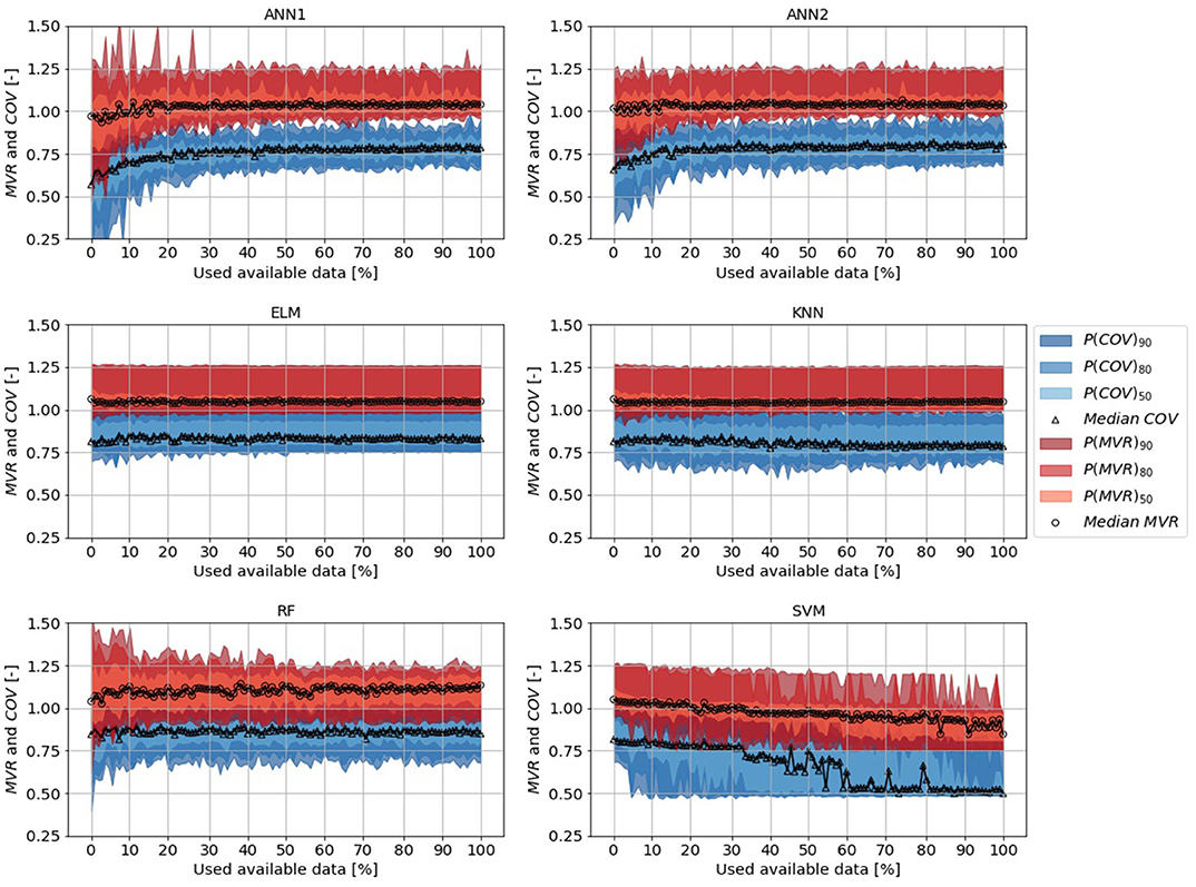
Figure 9. Dependence of mean volume reproduction (MVR)/temporal coverage (COV) and size of the training data set for different ML-algorithms in regional application. Uncertainty belts with different probabilities (50, 80, 90%) drawn for MVR in red scales, for COV in blue scales. The amount of training data has been raised incrementally to train the algorithms. Validation was performed on data sets in regional neighborhood of the training data sources in the Main basin.
In summary, the results showed that even with a small data set automated hydrograph separation could be performed in regional application. Neural network estimators (ELM, ANN1 and ANN2) and similarity-based estimators (KNN) performed best. Flood event duration estimates were afflicted with median bias of 20%. However, this mismatch of event duration did not result in a significant volume error (5% overestimation with ELM & KNN). Our results showed that a training data set of 35 manually separated flood events was needed to train ANNs, only the ELM and KNN should be used with less available data.
Based on this results, we asked if the algorithms could be applied to catchments of another basin, i.e., if the trained algorithms could be used in a trans-regional application. Likewise to the regional application, trained algorithms were used to estimate the time stamps of event begin and end of the floods events, but in this case for catchments in the Regen basin (Figure 2). The results of the trans-regional applications approved our findings of the regional application (Figure 10). Again, the ANN1 and ANN2 required 30-40% of the data to reach stable results. ELM and KNN, again, required less training data. Contrary to the regional application, the median MVR of the RF converged toward the optimum value of 1.0 with increasing data. Again, a training data set of approx. 35 flood events was sufficient to automate the task of hydrograph separation, even in a trans-regional application.
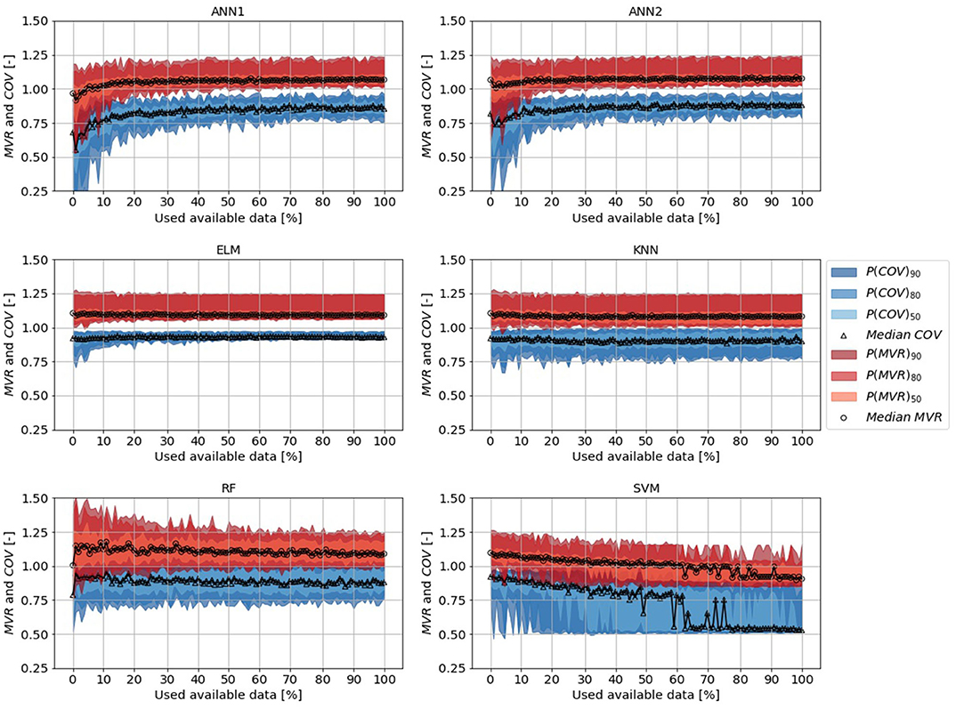
Figure 10. Dependence of mean volume reproduction (MVR)/temporal coverage (COV) and size of the training data set for different ML-algorithms in trans-regional application. Uncertainty belts with different probabilities (50, 80, 90%) drawn for MVR in red scales, for COV in blue scales. The amount of training data has been raised incrementally to train the algorithms. Validation was performed on data sets in the Regen basin.
4.3. Hydrograph Similarity
Our results showed that we could successfully apply an ELM or KNN trained with data from five basins in the Upper Main to other sub-basins within the same catchment and in another catchment. This brought up the question: why did it work? A trained, i.e., calibrated model can only be applied to other data without significant performance decrease if the patterns, i.e., variance, within the new data matches the training data. In the previous analysis we proved that our trained models could be applied without performance decrease. Hence, we made the hypothesis that the hydrographs within the training and validation data set, i.e., their variance was similar. As stated in section 3.1 the entropy concept is a good tool to assess the information, i.e., the variance within data sets. Hence, we analyzed the entropy of the training and validation data sets in order to test our hypothesis.
Although entropy quantifies the amount of information, it cannot assess the actual information and is, hence, not applicable to evaluate the equivalence of two data sets. But, if redundant information is added to a data set its entropy value decreases (compare section 2.3). We exploited this behavior of the entropy metric to assess the information equivalence of the training and validation data sets.
We incrementally enlarged a merged data set comprising hydrographs from the training data and one of the validation data sets (regional/transregional). In each step we added a single hydrograph to the data set and calculated the entropy value (Equation 1). First we added all training hydrographs, then we added the validation hydrographs. In order to assess the uncertainty of H, due to data availability we repeated this procedure 500 times, in each iteration only used 50% of the available data (randomly selected).
The results of this analysis supported our hypothesis (Figure 11). We found that H increased very quickly with only 2 or 3 data sets (actual position of HMax depending of selected hydrographs). After that H decreased, with some variance in its development due to data selection. Although variance was visible, HMax < 2.5 [bit] was never exceeded with the additional validation data, neither with the regional nor with the trans-regional data set. Note that HMax in this analysis was lower than the entropy values in section 3.1, because normalized hydrographs have been used to assess the information given to the ML-algorithms.

Figure 11. Development of entropy H for merged training and validation (regional REG/trans-regional TR) data sets. Median (black lines) and 90%-uncertainty belts calculated by randomly adding 50% of the available hydrographs per sub-basin to the merged data set.
5. Conclusions
In this article we demonstrated how machine learning can be used to automate the task of hydrograph separation from continuous time series. As predictor for the used ML-algorithm we used the ordinates of hydrograph, solely. This minimized the effort for data pre-processing. An analysis of entropy values and numerical experiments showed that only a short excerpt of the hydrograph (40 values, 20 prior, and another 20 succeeding the flood peak) were required for hourly discharge data.
Seven different ML-algorithms were trained with manually separated flood events and were applied locally, regionally and trans-regionally. All applications showed that machine learning was able to extract the relevant information (flood event duration and volume). In the local application, i.e., application of the trained algorithms to the same catchment, RF and SVM showed the best results. However, in regional and trans-regional application, i.e., application to other catchments than the training data source, estimators based on artificial neuronal networks (ELM, ANN with 1 hidden layer) and similarity based estimator (KNN) performed best.
Moreover, we demonstrated that the application of ML minimizes the effort for manual data pre-processing. For local application, data sets containing only 4–5 manually separated events were sufficient to transfer the experts knowledge to the algorithms. For a transfer of the trained algorithms to other catchments lacking training data, the manual effort increased slightly. In our applications, 35 events from 5 gauges, i.e., 7 events per gauge transferred the required amount of information to the ML-algorithm.
A striking observation was that the performance of flood event separation was comparable in local, regional and trans-regional application. With an assessment of information equivalence in the training and validation data sets we demonstrated that the variance of our predictors necessary to be applied to other data sets, could be covered with our training data set. The result of the analysis not only supported our hypothesis about information equivalence, but also provided an explanation why our approach to automation of event separation had a quicker learning process than other approaches like Thiesen et al. (2019). We excluded the majority of natural variance within the continuous time with the focus on the events we are interested in (via POT-method). From the time-stamp returned by POT we used the 40-discharge ordinates around the peak as predictors for the estimation of event beginning and end. With this procedure we focused the ML-algorithms on the shape of the flood event and trained it to identify its begin and end. Our results proved that this approach delivered good results and requires a minimum amount of manual work for training.
However, we have to focus on this topic in future works. We excluded the transfer to other climatic conditions and we excluded the impact of biased data. With additional data, taking more catchments into account, we want to test the application of trained algorithms to a wider range of possible applications than presented in this study. Moreover, more numerical experiments have to be carried out to evaluate the impact of the training data and choices made by the user, for example the chosen separation target. In this study we tried to separate the full flood event. However, other users might be interested in other tasks. Although our results are promising in this respect, further tests must be carried out.
Data Availability Statement
All datasets presented in this study are included in the article/Supplementary Material.
Author Contributions
This study was developed and conducted by both authors (HO and BM). HO provided the main text body of this publication which was streamlined by BM.
Funding
The financial support of the German Federal Ministry of Education and Research (BMBF) in terms of the project Wasserressourcen als bedeutende Faktoren der Energiewende auf lokaler und globaler Ebene (WANDEL), a sub-project of the Globale Ressource Wasser (GRoW) joint project initiative (Funding number: O2WGR1430A) for HO is gratefully acknowledged.
Conflict of Interest
The authors declare that the research was conducted in the absence of any commercial or financial relationships that could be construed as a potential conflict of interest.
Acknowledgments
The authors would like to thank the Bavarian Ministry of the Environment for providing the Data used in this study. We also like to thank Svenja Fischer for her feedback that helped to improve this work.
Supplementary Material
The Supplementary Material for this article can be found online at: https://www.frontiersin.org/articles/10.3389/frwa.2020.00018/full#supplementary-material
References
Addor, N., Nearing, G., Prieto, C., Newman, A. J., Le Vine, N., and Clark, M. P. (2018). A ranking of hydrological signatures based on their predictability in space. Water Resour. Res. 54, 8792–8812. doi: 10.1029/2018WR022606
Alpaydin, E. (2010). Introduction to Machine Learning. Adaptive Computation and Machine Learning, 2nd Edn. Cambridge, MA: MIT Press.
Blume, T., Zehe, E., and Axel, B. (2007). Rainfall–runoff response, event-based runoff coefficients and hydrograph separation. Hydrol. Sci. J. 52, 843–862. doi: 10.1623/hysj.52.5.843
Collischonn, W., and Fan, F. M. (2012). Defining parameters for Eckhardts digital baseflow filter. Hydrol. Process. 27, 2614–2622. doi: 10.1002/hyp.9391
Cortes, C., and Vapnik, V. (1995). Support-vector networks. Mach. Learn. 20, 273–297. doi: 10.1007/BF00994018
Cover, T. M., and Thomas, J. A. (2006). Elements of Information Theory, 2nd Edn. Hoboken, NJ: Wiley-Interscience.
Dahak, A., and Boutaghane, H. (2019). Identification of flow components with the trigonometric hydrograph separation method: a case study from Madjez Ressoul catchment, Algeria. Arab. J. Geosci. 12:463. doi: 10.1007/s12517-019-4616-5
Eckhardt, K. (2005). How to construct recursive digital filters for baseflow separation. Hydrol. Process. 19, 507–515. doi: 10.1002/hyp.5675
Elshorbagy, A., Corzo, G., Srinivasulu, S., and Solomatine, D. P. (2010a). Experimental investigation of the predictive capabilities of data driven modeling techniques in hydrology - Part 1: concepts and methodology. Hydrol. Earth Syst. Sci. 14, 1931–1941. doi: 10.5194/hess-14-1931-2010
Elshorbagy, A., Corzo, G., Srinivasulu, S., and Solomatine, D. P. (2010b). Experimental investigation of the predictive capabilities of data driven modeling techniques in hydrology - Part 2: application. Hydrol. Earth Syst. Sci. 14, 1943–1961. doi: 10.5194/hess-14-1943-2010
Fischer, S. (2018). A seasonal mixed-POT model to estimate high flood quantiles from different event types and seasons. J. Appl. Stat. 45, 2831–2847. doi: 10.1080/02664763.2018.1441385
Furey, P. R., and Gupta, V. K. (2001). A physically based filter for separating base flow from streamflow time series. Water Resour. Res. 37, 2709–2722. doi: 10.1029/2001WR000243
Gong, W., Yang, D., Gupta, H. V., and Nearing, G. (2014). Estimating information entropy for hydrological data: one-dimensional case. Water Resour. Res. 50, 5003–5018. doi: 10.1002/2014WR015874
Gonzales, A., Nonner, J., Heijkers, J., and Uhlenbrook, S. (2009). Comparison of different base flow separation methods in a lowland catchment. Hydrol. Earth Syst. Sci. 13, 2055–2068. doi: 10.5194/hess-13-2055-2009
Hall, F. R. (1968). Base-flow recessions-a review. Water Resour. Res. 4, 973–983. doi: 10.1029/WR004i005p00973
Hammond, M., and Han, D. (2006). Recession curve estimation for storm event separations. J. Hydrol. 330, 573–585. doi: 10.1016/j.jhydrol.2006.04.027
Huang, G.-B., Zhu, Q.-Y., and Siew, C.-K. (2004). “Extreme learning machine: a new learning scheme of feedforward neural networks, in 2004 IEEE International Joint Conference on Neural Networks (IEEE Cat. No.04CH37541), Vol. 2, 985–990 (Budapest). doi: 10.1109/IJCNN.2004.1380068
Kelleher, J. D., MacNamee, B., and D'Arcy, A. (2015). Fundamentals of Machine Learning for Predictive Data Analytics: Algorithms, Worked Examples, and Case Studies. Cambridge, MA; London: MIT Press.
Klaus, J., and McDonnell, J. J. (2013). Hydrograph separation using stable isotopes: review and evaluation. J. Hydrol. 505, 47–64. doi: 10.1016/j.jhydrol.2013.09.006
Lyne, V., and Hollick, M. (1979). “Stochastic time-variable rainfall-runoff modelling, in Institute of Engineers Australia National Conference (Barton, ACT: Institute of Engineers Australia), 89–93.
Mei, Y., and Anagnostou, E. N. (2015). A hydrograph separation method based on information from rainfall and runoff records. J. Hydrol. 523, 636–649. doi: 10.1016/j.jhydrol.2015.01.083
Merz, R., and Blöschl, G. (2009). A regional analysis of event runoff coefficients with respect to climate and catchment characteristics in Austria. Water Resour. Res. 45. doi: 10.1029/2008WR007163
Merz, R., Blöschl, G., and Parajka, J. (2006). Spatio-temporal variability of event runoff coefficients. J. Hydrol. 331, 591–604. doi: 10.1016/j.jhydrol.2006.06.008
Minns, A. W., and Hall, M. J. (2005). “Artifical neuronal network concepts in hydrology, in Encyclopedia of Hydrological Sciences, Vol. 1, ed M. G. Anderson (Chichester: Wiley), 307–319. doi: 10.1002/0470848944.hsa018
Mount, N. J., Maier, H. R., Toth, E., Elshorbagy, A., Solomatine, D., Chang, F.-J., et al. (2016). Data-driven modelling approaches for socio-hydrology: opportunities and challenges within the Panta Rhei science plan. Hydrol. Sci. J. 8, 1–17. doi: 10.1080/02626667.2016.1159683
Mountrakis, G., Im, J., and Ogole, C. (2011). Support vector machines in remote sensing: a review. ISPRS J. Photogrammetry Remote Sens. 66, 247–259. doi: 10.1016/j.isprsjprs.2010.11.001
Oppel, H., and Schumann, A. (2020). Machine learning based identification of dominant controls on runoff dynamics. Hydrol. Process. 34, 1–16. doi: 10.1002/hyp.13740
Pedregosa, F., Varoquaux, G., Gramfort, A., Michel, V., Thirion, B., Grisel, O., et al. (2011). Scikit-learn: machine learning in python. J. Mach. Learn. Res. 12, 2825–2830.
Scott, D. W. (1979). On optimal and data-based histograms. Biometrika 66, 605–610. doi: 10.1093/biomet/66.3.605
Shannon, C. E. (1948). A mathematical theory of communication. Bell Syst. Tech. J. 27, 379–423. doi: 10.1002/j.1538-7305.1948.tb01338.x
Sharma, A., and Mehrotra, R. (2014). An information theoretic alternative to model a natural system using observational information alone. Water Resour. Res. 50, 650–660. doi: 10.1002/2013WR013845
Shortridge, J. E., Guikema, S. D., and Zaitchik, B. F. (2016). Machine learning methods for empirical streamflow simulation: a comparison of model accuracy, interpretability, and uncertainty in seasonal watersheds. Hydrol. Earth Syst. Sci. 20, 2611–2628. doi: 10.5194/hess-20-2611-2016
Solomatine, D. P., and Ostfeld, A. (2008). Data-driven modelling: some past experiences and new approaches. J. Hydroinform. 10, 3–22. doi: 10.2166/hydro.2008.015
Stewart, M. K. (2015). Promising new baseflow separation and recession analysis methods applied to streamflow at Glendhu catchment, New Zealand. Hydrol. Earth Syst. Sci. 19, 2587–2603. doi: 10.5194/hess-19-2587-2015
Su, N. (1995). The unit hydrograph model for hydrograph separation. Environ. Int. 21, 509–515. doi: 10.1016/0160-4120(95)00050-U
Tabari, H., Kisi, O., Ezani, A., and Talaee, P. H. (2012). SVM, ANFIS, regression and climate based models for reference evapotranspiration modeling using limited climatic data in a semi-arid highland environment. J. Hydrol. 444–445:78–89. doi: 10.1016/j.jhydrol.2012.04.007
Tallaksen, L. (1995). A review of baseflow recession analysis. J. Hydrol. 165, 349–370. doi: 10.1016/0022-1694(94)02540-R
Thiesen, S., Darscheid, P., and Ehret, U. (2019). Identifying rainfall-runoff events in discharge time series: a data-driven method based on information theory. Hydrol. Earth Syst. Sci. 23, 1015–1034. doi: 10.5194/hess-23-1015-2019
Weiler, M., Seibert, J., and Stahl, K. (2017). Magic components-why quantifying rain, snowmelt, and icemelt in river discharge is not easy. Hydrol. Process. 32, 160–166. doi: 10.1002/hyp.11361
Wittenberg, H., and Aksoy, H. (2010). Groundwater intrusion into leaky sewer systems. Water Sci. Technol. 62, 92–98. doi: 10.2166/wst.2010.287
Wolpert, D. H., and Macready, W. G. (1997). No free lunch theorems for optimization. IEEE Trans. Evol. Comput. 1, 67–82. doi: 10.1109/4235.585893
Yu, P.-S., Yang, T.-C., Chen, S.-Y., Kuo, C.-M., and Tseng, H.-W. (2017). Comparison of random forests and support vector machine for real-time radar-derived rainfall forecasting. J. Hydrol. 552, 92–104. doi: 10.1016/j.jhydrol.2017.06.020
Keywords: flood event separation, information extraction, time series, automation, data preprocessing
Citation: Oppel H and Mewes B (2020) On the Automation of Flood Event Separation From Continuous Time Series. Front. Water 2:18. doi: 10.3389/frwa.2020.00018
Received: 26 March 2020; Accepted: 17 June 2020;
Published: 28 July 2020.
Edited by:
Chaopeng Shen, Pennsylvania State University (PSU), United StatesReviewed by:
Jie Niu, Jinan University, ChinaMeysam Salarijazi, Gorgan University of Agricultural Sciences and Natural Resources, Iran
Copyright © 2020 Oppel and Mewes. This is an open-access article distributed under the terms of the Creative Commons Attribution License (CC BY). The use, distribution or reproduction in other forums is permitted, provided the original author(s) and the copyright owner(s) are credited and that the original publication in this journal is cited, in accordance with accepted academic practice. No use, distribution or reproduction is permitted which does not comply with these terms.
*Correspondence: Henning Oppel, aGVubmluZy5vcHBlbEBydWIuZGU=