
95% of researchers rate our articles as excellent or good
Learn more about the work of our research integrity team to safeguard the quality of each article we publish.
Find out more
ORIGINAL RESEARCH article
Front. Water , 21 April 2020
Sec. Water and Hydrocomplexity
Volume 2 - 2020 | https://doi.org/10.3389/frwa.2020.00008
This article is part of the Research Topic Model-Data Fusion in Hydrology View all 6 articles
 Silvio J. Gumiere1*
 Matteo Camporese2
 Anna Botto2
 Jonathan A. Lafond1
 Claudio Paniconi3
 Jacques Gallichand1
 Alain N. Rousseau3
Real-time monitoring of soil matric potential has now become a common practice for precision irrigation management. Some crops, such as cranberries, are susceptible to both water and anoxic stresses. Excessive variations in soil matric potential in the root zone may reduce plant transpiration, due to either saturated or dry soil conditions, thereby reducing productivity. A timely supply of the right amount of water is, therefore, fundamental for efficient irrigation management. In this paper, we compare the capabilities of a machine learning-based model and a physics-based model to predict soil matric potential in the root zone. The machine learning model is a random forest algorithm, while the physics-based model is a two-dimensional solver of Richards equation (HYDRUS 2D). After training and calibration on a dataset collected in a cranberry field located in Québec (Canada), the performance of the two models is evaluated for 30 different time frames of 72-h soil matric potential forecasts. The results highlight that both models can accurately forecast the soil matric potential in the root zone. The machine learning-based model can achieve better performance when compared to the physics-based model, but forecasting accuracy decreases rapidly toward the end of the 72-h lead time, while the error for the Richards equation-based model does not increase with time and remain small compared to the typical measurement error.
Meeting future food demands for a rising global population while minimizing environmental impacts remains a challenge, for which precision irrigation strategies will play a critical role (Provenzano and Sinobas, 2014). Precision irrigation is based on real-time measurements of soil moisture conditions and the capacity of models to predict the amount to be applied for irrigation scheduling (Autovino et al., 2018). When applying water-saving irrigation strategies, one must observe water stress indicators, such as soil water content, soil matric potential in the root zone, leaf water potential, etc. These indicators may help to prevent water stress conditions and excessive water use (Rallo et al., 2014). However, they do not inform growers on how much water is needed to bring the plant root zone to optimal conditions. Besides, most of the time, when the plant water stress can be observed, it is already too late to act (Rekika et al., 2014), especially in highly sensitive crops such as lettuce, tomatoes and cranberries (Lafond et al., 2015; Pelletier et al., 2017). That is why soil-water-plant-atmosphere models (SWPA) are often used to provide information on the soil and plant water status (Minacapilli et al., 2009; Cammalleri et al., 2013; Aguilera and Ruiz-Valenzuela, 2019). Several physically-based and process-based models, such as HYDRUS (Autovino et al., 2018) and CATHY (Camporese et al., 2015), are currently used to describe water processes in the SWPA continuum. After appropriate calibration and validation, these models can be used to support irrigation water management, providing not only the timing of irrigation, but also the amount of water needed, therefore helping to increase productivity and reduce water use. For example, Bigah et al. (2019) proposed a process-based model to predict the water needs for different cranberry farm operations such as irrigation, frost protection and harvest. Rekika et al. (2014) proposed an analytical model to estimate soil critical matric potential thresholds for irrigation management for various highly sensitive crops (onions, celery, and baby spinach seed germination).
In the last few years, along with physics-based models, many machine learning (ML) based models have been developed and applied to water management. Artificial Neural Networks (ANN) have been used to model the water table dynamics of various agricultural systems (Dibike and Coulibaly, 2006; Yoon et al., 2011). Li et al. (2016) have compared the capacity of Random Forest (RF) and ANN models to predict lake water levels. The results demonstrated that the RF model has superior predictive capabilities with fewer parameters and training time. Decision tree-based models have been successfully applied in groundwater hydrological modeling (Singh et al., 2014; Wang et al., 2018). Marques et al. (2005) used ML algorithms to optimize water supply for crops at different growing stages, given the water cost, the market price, cost of irrigation, crop expenses, and expected yield reduction due to under- or over-irrigation throuhout the entire growing period. The resulting optimization models were incorporated into a decision support system (DSS) for precision irrigation, but did not account for field-specific characteristics. Literature also comments on models for determining irrigation needs based on field-specific data. For example, Hedley et al. (2013) used ML to predict soil water status and water table depth based on soil resistivity mapping. Smith and Peng (2009) used ML to classify soil textural composition based on infrared measurements as an input to a deficit irrigation control system. However, none of these studies have compared the performance between physics-based and ML-models for predicting soil water status using the same dataset.
Given the increased popularity of ML approaches, the main objective of this paper was to test the efficiency of a physics-based model, HYDRUS-2D, and a ML-based model, a Random Forest (RF) model, in predicting soil water status for a highly sensitive and valuable crop. Using a dataset collected at an experimental site in Québec (Canada), HYDRUS and RF were used, after appropriate calibration and training, to predict the water status in the root zone with up to a 72-h lead time, in the context of real-time precision irrigation management. The comparison between the two approaches was made from the perspective of a grower or an irrigation manager, who typically only measures soil matric potential at one location to manage irrigation in their crop-fields.
The study area was located on a cranberry farm, under a warm and humid summer climate, near Québec City, Québec, Canada (46°14′N, 72°02′W). The average rainfall in June and September is 48.0 mm and 70.6 mm, while the average temperatures are 17.1 and 13.3°C, respectively. The location of the farm is shown in Figure 1, and the studied cranberry fieldis ~18 ha (40-m wide by 450-m long). This site is equipped with a subsurface drainage system with four drainage pipes, equally spaced at 12 m, at an average depth of 0.9 m below the soil surface. These subsurface drains, which are designed to maintain a 0.6-m deep water table throughout the field, discharge into a control chamber south of the site. This setup is designed to ensure adequate moisture conditions, ideally keeping the plant root zone between −6.5 and −4 kPa. Three PVC pipes were inserted vertically at mid-spacing between the subsurface drains, serving as observation wells for water table measurements. The site was also equipped with a rain gauge.
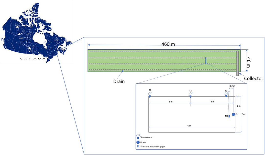
Figure 1. Site localization in Quebec (Canada) and location of the tensiometers (T1, T2, and T3 installed at 10 cm bellow the soil surface), the water table pressure gage (N3) and the drains within the cranberry field.
Cranberry (Vaccinium macrocarpon Ait.) is a high-value perennial crop that has historically been grown on wetlands (peat soils), but is also commonly cultivated on sandy anthropogenic soils. The cranberries require about 60 mm of water per month during the growing season in Québec (Pelletier et al., 2015). The water table must be controlled during the growing season because too dry or too wet conditions can adversely affect cranberry growth and root development (Périard et al., 2017). A water table depth between 0.3 and 0.5 m for sandy soils and around 0.6 m for peat soils can meet cranberry water requirements by capillary rise (Périard et al., 2017). A soil with high a hydraulic conductivity is preferred to maintain optimal water conditions for cranberry growth by water table control or irrigation (Gumiere et al., 2017). As mentioned previously, for cranberry production in Québec, the optimal range of soil water matric potential in the root zone (i.e. 10-cm deep) is between −6.5 and −4.0 kPa (Caron et al., 2017). Thus, matric potential and hydraulic conductivity represent the soil properties with the largest impact on cranberry yields.
Precipitation was measured every 15 min using a rain gauge (WatchDog 1120 Rain Gauge, Spectrum Technology, Inc., IL US) combined with an ST-4 Hortau datalogger (Lévis, Québec, www.hortau.ca). In summer, sprinkler irrigation was used for cooling crops. Thus, the rain gauge also measured the amount of irrigation. The total precipitation used in this study is the sum of irrigation and rainfall.
Water table (WT) depth was continuously measured using a submersible pressure transducer (TDH80, Transducersdirect Inc., Ellington Court Cincinnati, Ohio, USA) and a datalogger (ST-4, Hortau Inc., Lévis, Québec, Canada). This sensor automatically corrects data for atmospheric pressure. The soil surface was the elevation datum for the pressure depth measurements. Data were collected every 15 min and sent wirelessly to Hortau's Irrolis (Irrolis 3 v.3.5.1, Hortau Inc., Lévis, Québec, Canada) website. For the physics-based model, WT values were only used to assign the boundary conditions at the drain location.
Soil matric potential (SMP) was measured continuously with commercial tensiometers (HXM-80, Hortau Inc., Lévis, Québec, Canada) connected to the same ST-4 datalogger. The tensiometers were located at three positions (T1, T2, T3 at a depth of 10 cm), transversally to the subsurface drain, as shown in Figure 1. Data were collected every 15 min and transferred to Hortau's Irrolis (Irrolis 3 v.3.5.1, Hortau Inc., Lévis, Québec, Canada) website. Missing SMP values were interpolated from existing measurements using cubic splines (Moritz and Bartz-Beielstein, 2017). Hourly SMP values used in this study are the measured average of four 15-min measurements. Figure 2 shows all the hydrometeorological, i.e., precipitation, WT and SMP.
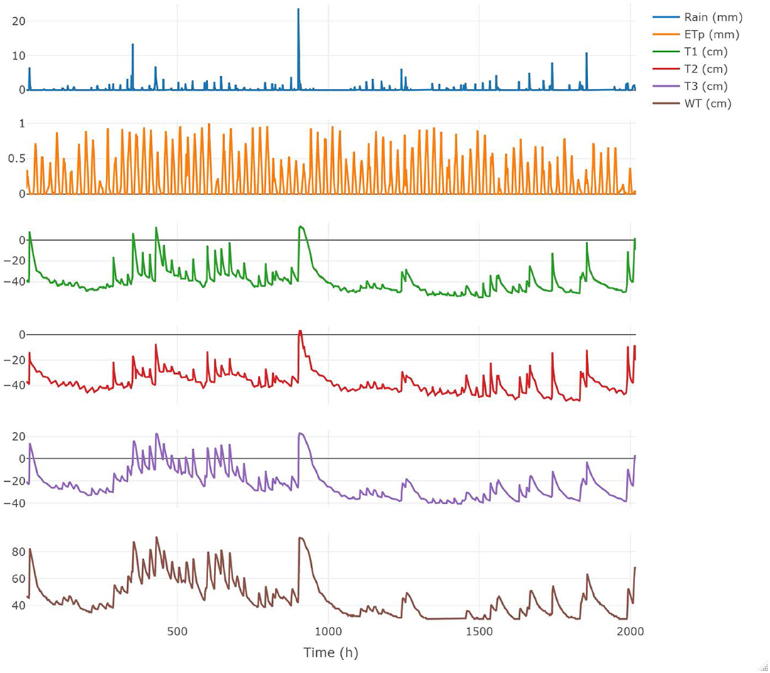
Figure 2. Observed hydrometeorological data collected in the study area. From the top, we report rainfall, potential evapotranspiration, soil matric potential measured at T1, T2, and T3 locations, and water table near the drain.
Random Forest (RF) is a supervised ML method with multiple building blocks (decision trees) producing an ensemble of predictive models (Rodriguez-Galiano et al., 2014). Amongst supervised ML algorithms, RF has proven to be suitable for either classification or regression, depending on the nature of the targeted variable. For simulating soil matric potential in the root zone, we only used regression trees (RT).
The regression algorithm is built around a set of hierarchically structured restrictions, sequentially applied to a root node up to terminal nodes of the decision tree (Breiman, 2001). To prevent correlations between the different RTs, RF develops each tree independently using different bootstrap samples extracted from the learning dataset and a subset of randomly selected variables out of the predictive variables (Breiman, 2001). Specifically, the RF builds each tree by making them grow from two-thirds of each bootstrap sample (in-bag). About one-third of the samples are excluded from the bootstrap sample (out-of-bag) for a non-biased estimation of the regression error. A prediction of the out-of-bag (OOB) data is generated for each tree. These predictions are subsequently averaged to obtain an estimation of the error rate of the OOB. The generalization error of the RF model depends on the weight of the individual trees and the correlations between them (Qu et al., 2019). The building of a RT follows a recursive binary partition approach starting at the root node and divides the non-correlated variables into two new branches. This recursive division is performed on the dependent variable as a function of the most significant independent variable, leading to the best ensemble of homogeneous populations. Each node is then divided using the most homogeneous population among the subsets of predictive variables selected randomly at the node. This division process continues until a predefined number of observations at the terminal node (node size) is reached. The result obtained using the RF is, in the case of a regression, an average of the predictions from all decision trees.
The RF regression algorithm can be summarized into three basic steps as follows (Breiman, 2001):
• Different bootstrap samples Wi (i = bootstrap iteration) are randomly drawn from the original dataset W. Two-thirds of the samples are included in a bootstrap sample and one-third as the OOB samples. Each tree is constructed to correspond to a particular subset of the bootstrap.
• At a node in each tree, a new split is randomly selected from all indices, and the input variable with the lowest mean squared error (MSE) is chosen as the splitting criterion of the regression tree.
• The data splitting process at each internal node is repeated according to the above steps until all randomized trees have been grown, and a stop condition is achieved.
The final results of the regression are calculated as follows, where N stands for the number of trees in the forest and Tn represents a tree:
The RF-model was implemented in R Development Core Team (2010) using the package caret (Kuhn, 2020). Soil matric potential (SMP) at the root zone was predicted hourly from 1 to 72 h ahead. As input, we considered rainfall (P), potential evapotranspiration (ET0) and SMP at the T1 position only (Figure 1) in the root zone of previous time steps. The T1 position was chosen because most growers typically measure soil matric potential in one location only, and the most significant position in cranberry fields is indeed in the middle of two drains.
The model was built with separate combinations of input variables. Lag times of input variables were generated by means of the sliding window method (Brédy et al., 2020), which allowed us to restructure the time series of P, ET0, and SMP as a supervised learning problem by using a size of the lag (d) equal to 168 h. This lag size was chosen to consider the influence of the SMP values at position T1 over the previous 168-h time period on the predictions. Therefore, we constructed the ML-based model maps an input window of width d into an individual output value y. The model predicts the SMP values at the T1 position (yi, t+j, with j the time step forecast) using the window: (xi, t+j, xi, t+j−1, …,xi, t, …, xi, t−d+1, xi, t−d) for P and ET0 and (yi, t, …, yi, t−d+1, yi, t−d) for the antecedent SMP value. Multi-step forecasts from 1 to 72-time steps were used for forecasting the SMP value in the root zone.
Evapotranspiration (ET0) was estimated using the formula proposed by Baier and Robertson (1965):
Where Ra is the extraterrestrial radiation (cal cm−2 d−1), ET0day is the daily evapotranspiration (mm d−1) and Tmax and Tmin are daily maximum and minimum emperatures (°C).
The temperatures were measured using the Hortau's weather station, which includes the WatchDog 2900ET (Spectrum Technology, Inc., IL USA). To obtain hourly ET (used as input), the results from Baier and Robertson's formula were multiplied by a ratio of extraterrestrials radiations for hourly (Rh) and daily (Rd) periods using the equation, . The extraterrestrial radiation for the daily and hourly periods were estimated using the equations of Allen et al. (1998), which for each day of the year and for different latitudes, can be estimated from the solar constant, Gsc = 4.92 MJm−2d−1.
Because of computational time constraints, the number of decision trees (ntree) was set to 200; as reported by Rodriguez-Galiano et al. (2014) and (Brédy et al., 2020), the gain in accuracy is negligible for ntree > 200.
The experimental dataset consisted of 2,000 hourly observations for each variable (P, ET0, and SMP at T1 position) ranging from July to September 2018. This dataset was split by the holdout method, using the “CreateDataPartition” caret package function Kuhn (2020) in two subsets: a training subset, which contained 70% of data randomly selected for each dataset and the remaining 30% that were used as test subset. For each step-ahead prediction,this data division was repeated 30 times using a uniform distribution. This allowed the models to be trained and validated with a total of 30 different training and test subsets for each training pattern (t + 1 to t + 72) and to estimate the variability of their results.
The calibration procedure aims to optimize a set of model parameter values that enable the model to map the relationship between the inputs and outputs of a given dataset (Wu et al., 2014). For the RF method, two parameters (ntree and mtry) were assigned using results and recommendations from the literature: 200 trees and 1/3 of the predictive variables (Liaw and Wiener, 2002), respectively. The model was trained to determine the optimal parameter values that minimize the training error. The test data were used to independently assess the generalization ability of the trained model, an essential step to evaluate the model quality and accuracy with data that were not used in training.
Assuming that the air phase does not affect the liquid flow processes and that thermal gradients are negligible, the water movement in partially saturated porous media can be described by Richards equation (Richards, 1931):
where Sw = θ/ϕ is water saturation, θ and ϕ being the volumetric soil water content and porosity [/], respectively, Ss is the specific storage coefficient [L−1], [L−1], ψ is the pressure head [L], t is time [T], ∇ is the gradient operator, Ks is the saturated hydraulic conductivity tensor [L/T], [L/T], Kr is the relative hydraulic conductivity function [/], is the vertical direction vector, z is the vertical coordinate directed upward [L], and qs represents a sink term [L3/L3T] [L3/L3T] accounting for evapotranspiration.
The unsaturated hydraulic properties are taken into account by means of the van Genuchten functions Sw(ψ) and Kr(ψ)Kr(ψ) (Van Genuchten, 1980):
where Swr = θr/ϕ is the residual water saturation, with θr the residual water content, α is an empirical constant [L−1] related to the inverse of the air entry suction, while the dimensionless shape parameters n and m are linked by the expression m = 1−1/n. These parameters are often referred to as the van-Genuchten Mualem (VGM) parameters.
The sink term (qs) in Richards equation accounts for depth-dependent root water uptake. The potential evapotranspiration (ET0) is distributed across the root depth according to a root distribution function. Actual evapotranspiration depends on soil water content and, hence, on the soil matric potential in the root zone. If the soil is dry, vegetation can experience water stress, and transpiration would reduce to limit water losses; in nearly saturated conditions, the low availability of oxygen to roots might also cause a decrease in the transpiration rate. We modeled the effect of low and high soil moisture on root water uptake by multiplying the potential root water uptake by a reduction function, αrw (Feddes et al., 1974). The reduction function, commonly referred to as Feddes function, is zero at pressure heads higher or equal to ψ1, close to saturation when oxygen stress is inhibiting root water uptake. As ψ decreases, αrw is assumed to increase linearly up to 1 at the anaerobiosis point (ψ2). When pressure head falls below ψ3, associated with incipient water stress, transpiration is assumed to decrease linearly, reaching zero at the wilting point, ψ4. Between ψ2 and ψ3 the soil is under well-watered conditions and roots can take up water at their potential rate (i.e., αrw = 1).
Equation (1) is solved with the HYDRUS-2D (Šimunek et al., 2003) using Galerkin-type linear finite element schemes.
A vertical cross-section of a half cranberry field is simulated. The domain (Figure 1) is 1-m deep and 6-m wide with a subsurface drain at one end and the middle of the field at the other end. The computational domain represents mid-drain spacing. It is discretized with a 2D finite element mesh of 4,000 nodes and 8,000 elements. No-flow boundary conditions are assumed on the sides and bottom of the domain, while seepage face or Dirichlet boundary conditions, according on whether the water table is above or below the drain, respectively, are used to represent the drain. At the surface, measured precipitation and estimated ET0 rates are imposed.
A hydrostatic profile corresponding to a water table of 0.5 m below the surface was used as initial condition for all the simulation scenarios. In addition, a warm-up period of five days was always applied before the start of each calibration; such a period was found to be sufficient to dissipate the influence of the arbitrary initial conditions.
The parameters of the Feddes model for cranberries are known (Caron et al., 2017), with values for ψ1, ψ2, ψ3, and ψ4 of −0.1, −0.45, −0.75, and −3.0 m, respectively. The maximum rooting depth is 0.15 m and the root distribution is linear. The VGM soil parameters (Ks, ϕ, θr, α, and n) were calibrated according to the procedure described in the next section.
The model was first calibrated using the entire data set of SMP within the root zone measured in the T1 position (Figure 1). This calibration was carried out to evaluate the possibility of obtaining a well performing model. In order to verify the accuracy and the physical validity of this simulation, we show in Figure 3 the performance of the model for all the three tensiometers available, although T2 and T3 were not used for calibration. To minimize the RMSE (Equation 5) between observed and simulated soil matric potentials, we used the Marquardt-Levenberg parameter estimation technique implemented in HYDRUS (Šimu°nek and Hopmans, 2002).
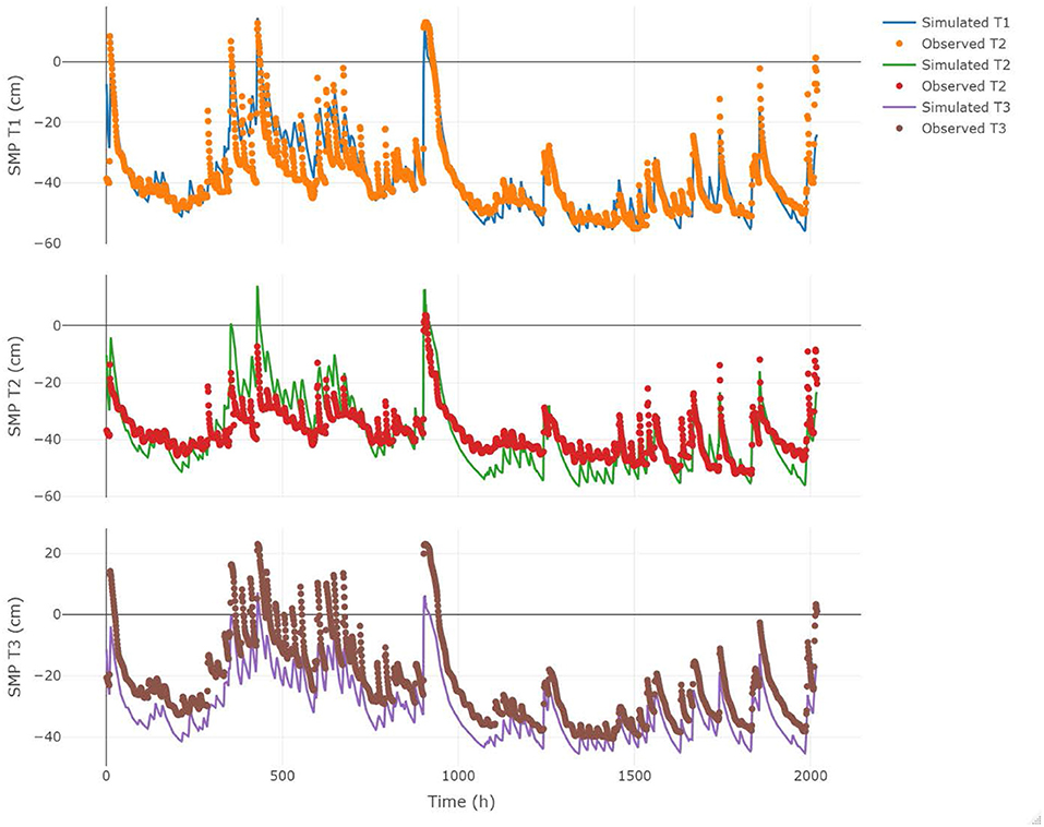
Figure 3. Simulation results of the physics-based model for the calibration run using the entire time series of soil matric potential measured at T1 location. Results for T2 and T3 are shown for validation. RMSE values for T2 and T3 are 7.68 and 9.4 cm; NSE values for T2 and T3 are 0.66 and 0.21 and R2 values 0.72 and 0.94, respectivelly.
The same optimization method was used to calibrate the soil parameters in 30 different simulation scenarios, whereby a time window of 408 h was used for calibration and the subsequent 72 h for forecasting, in order to consistently compare the forecasting capacity of the calibrated model with that of the trained ML algorithm.
Three statistical evaluation criteria were used to evaluate both models predictive power and efficiency:
(1) The root mean square error (RMSE):
(2) The Nash-Sutcliffe efficiency (NSE):
And (3) the coefficient of determination (R2):
where ỹ average simulated value, ŷi are the observed data, yi the simulated data, the mean of observed values and N the number of observations. For a model to yield a good fit between simulated and observed data the RMSE should be close to zero, while NSE and R2 close to one. In this study, RMSE and NSE statistics are used to measure the model performance for forecasting SMP fluctuation whereas R2 is used to analyze the linear regression goodness of fit between observed and simulated data.
Figure 3 shows the calibration results for tensiometer T1, ranging from 0 to 2018 h, between July 2018 and September 2018. The resulting RMSE, NSE and R2 values, obtained during training, are 6.18 cm, 0.74, and 0.79, respectively. They suggest a very good agreement between observed and simulated values of SMP; giving confidence about the possibility of successfully calibrating the model and the subsequent comparison with the ML-based model.
Figure 4 shows the comparison between simulated and observed SMP time series at the T1 location (root zone) for 27 of the 30 scenarios. Figure 5 presents a scatter plot of simulated vs. observed SMP values at the same location for the same scenarios. The temporal dynamics following calibration is well represented by the physics-based model, showing average performance criteria for RMSE, NSE and R2 of 6.46 cm, 0.72 and 0.82, respectively. Three simulations, out of the 30 scenarios, did not converge due to numerical instabilities, corresponding to 10% of the runs. The reasons for such instabilities can probably be found in a complex interplay of initial conditions (a 2-days warm-up used for every simulation) and soil parameters whose search space was limited and therefore did not allow for a comprehensive representation of the whole parameter space. Another possible explanation is that, due to the very short calibration windows (i.e., 360 h) which did not represent the total range of possible situations (i.e., from very dry to very wet periods), the calibration would have needed a larger parameter space to reasonably simulate the observed values.
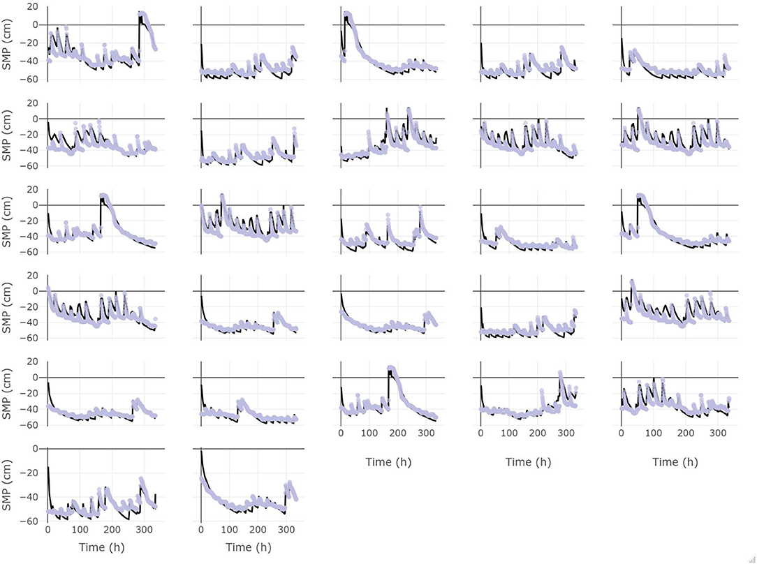
Figure 4. Comparison between simulated and observed SMP in time for 27 of the 30 initial windows of randomly chosen scenarios, gray full points represents observed values and full black line the simulated values of SMP.
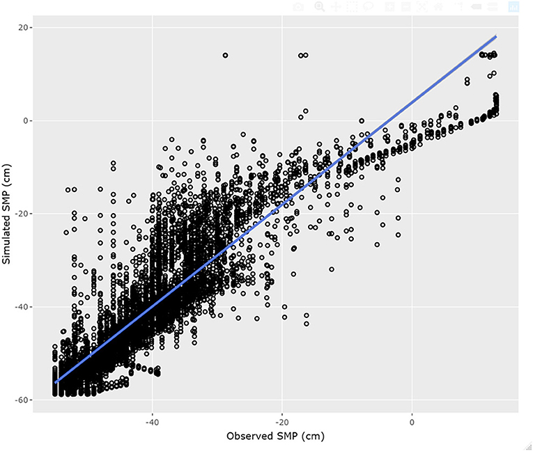
Figure 5. Scatter plot of observed vs. simulated SMP at the root zone for 27 of the 30 scenarios completed by the physics-based model using the calibration dataset. The blue line represents the fitted linear model between simulated and observed values.
Figure 6 shows box plots of the calibrated van Genuchten-Mualem (VGM) parameters and saturated hydraulic conductivity for the 27 scenarios that converged. The VGM parameters were calibrated individually for each scenario using the Marquardt-Levenberg type parameter optimization algorithm for inverse modeling included in HYDRUS-2D. The initial VGM parameters were measured in the field and were fixed to the same value for each scenario (θr = 0.072, θs = 0.423, α = 0.03 cm−1, n = 1.56, m = 1−1/n, and Ksat = 19.62cm/h). The resulting variability of the soil hydraulic properties (VGM) is relatively large, with some runs having parameters equal to the lower or upper bounds, an additional clue of a limited search space that could have led to the three simulations not converging. Once again, this variation may be due to the initial small windows selected, making the soil hydric condition very different from window to window, and causing a wide range of soil parameters required for simulating the water dynamics. Another possible explanation could be hysteresis, not accounted for in the model, due to the fact that for some windows the system is mainly draining while for others the water table is mainly rising.
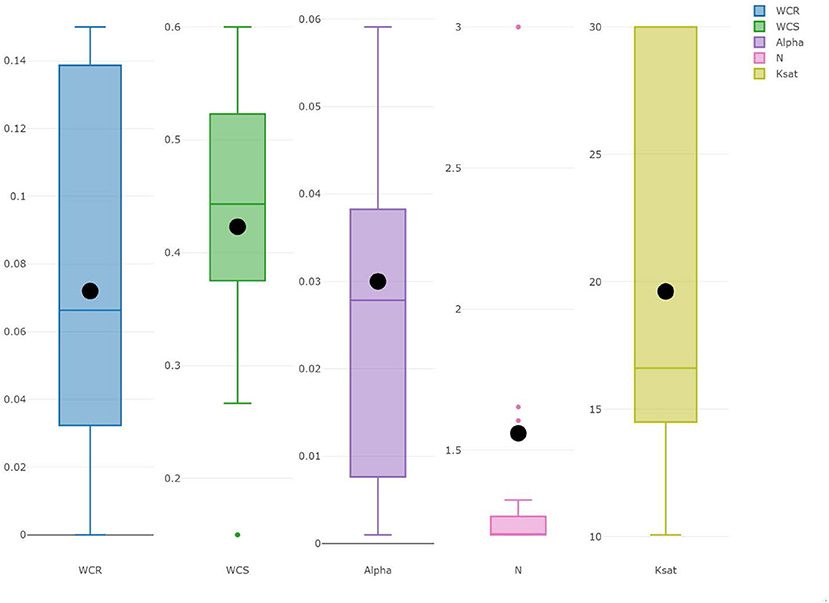
Figure 6. Boxplot of soil hydraulic parameters for the 27 scenarios completed by the physics-based model, full circles in black indicate the initial parameters.
Figure 7 shows the scatter-plot of the relationship between observed and simulated SMP values for the forecasting period for all the 27 successful scenarios. The model performance is still very good, with RMSE = 5.72cm, NSE = 0.78, R2 = 0.82 indicating an excellent agreement between simulated and observed values of SMP in the forecasting period.
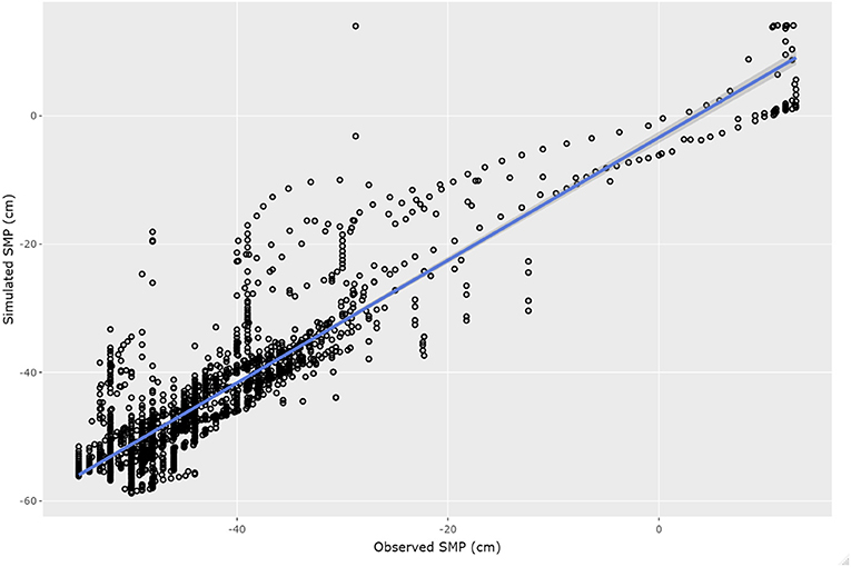
Figure 7. Scatter plot of observed and simulated soil matric potential in the root zone for 27 of the 30 scenarios completed by the physics-based model using the validation dataset (forecasting period). The blue line represents the fitted linear model between simulated and observed values.
Figure 8 shows the RMSE over time for the forecasting period (from 1 to 72 h). The RMSE values remain limited within a range of 3–8 cm, without apparent increasing or decreasing trend, suggesting a random distribution of errors.
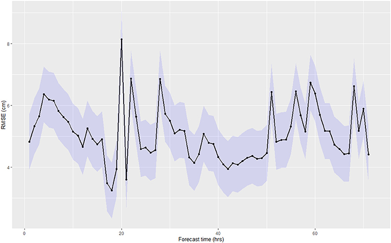
Figure 8. Temporal dynamics of the RMSE for the physics-based model.
Figure 9 shows the out-of-the-bag (OOB) squared error over the ntree parameter for the testing period. For ntree > 50 the error is constant, showing no gain for ntree > 200.
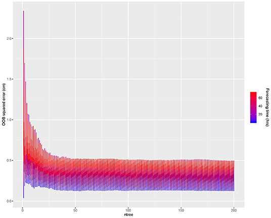
Figure 9. Out-of-the-bag error as a function of the ntree RF parameter. The barcolor represents the forcasting time.
Figure 10 shows the scatter plot between observed and simulated SMP values for the 30 testing periods, i.e., 30% of the 408 h of data for each period. The performance metrics over all simulation scenarios are RMSE = 8.49cm, NSE = 0.55, and R2 = 0.58, showing a drastic reduction of ML-model efficiency for testing.
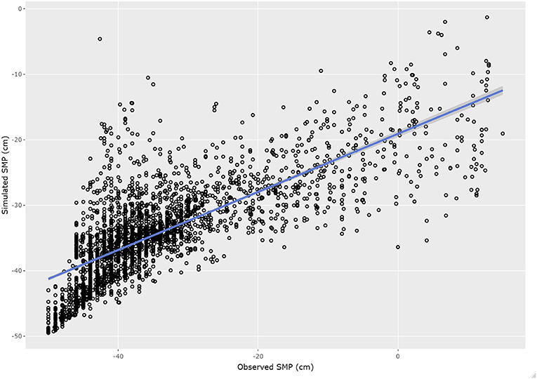
Figure 10. Scatter plot of simulated and observed soil matric potential in the root zone for the ML model in the forecasting period. The blue line represents the fitted linear model between simulated and observed values.
Figure 11 shows the RMSE as a function of forecasting time. RMSE values vary from 2 to 8 cm, with a clear increasing trend over time, confirming a strong reduction of the ML-based model prediction capabilities as the forecasting time increases.
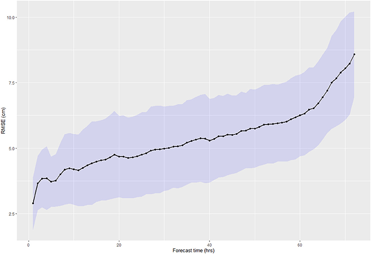
Figure 11. Temporal dynamics of the RMSE for the ML model.
Both physics-based and ML-based models were used here to predict SMP values in the root zone of a cranberry field. The ML-based model shows a strong dependency on the forecasting period. This dependence is somehow expected because the model is based on an autoregressive relationship of the input variables. The RMSE values increased quickly in the first 3 h and leveled off from hours 20 to 60 in the forecasting period, before increasing again. These results are consistent with the findings by Nayak et al. (2006), who showed that the performance of ML-based models (ANN, RF, Gradient Boosting) was better for shorter lead times, but became worse as the prediction time increased. Compared with ANN models, the tree-based ones do not stay in a local minimum which causes over-adjustment during the training period (Maier et al., 2010). Also, decision-tree models are not affected by missing and correlated data and they have been widely used in modeling natural phenomena.
For the physics-based model, the RMSE values appear to be completely random, mostly oscillating between 4 and 7 cm, with a single peak reaching 8 cm around 20 h of the forecasting period. Interestingly, after 50 h in the forecasting period, the physics-based model shows better performance than the ML-based model. However, overall, both models display good performances in terms of RMSE and NSE values during the calibration and validation (training and testing, for ML) steps, which indicates that both models can provide satisfactory forecasting SMP values for irrigation management. Indeed, for cranberries, an error of less than 10 cm in SMP prediction is acceptable for irrigation management (Pelletier et al., 2017), considering a period of reaction of 24 or less for the irrigation to be activated into the concerned fields.
The physics-based model has the advantage of being able to consistently represent the water dynamics over the entire domain, not only where it was calibrated, as is the case for the ML-based model for which no extrapolation is possible beyond the range of observed values. On the other hand, physics-based models need additional efforts to assign proper initial and boundary conditions, as well as parameter heterogeneity, in order to represent the soil water dynamics accurately. Also, physics-based models would likely need to be constantly calibrated as new data are collected to maintain an effective prediction capability. For this study, where the time windows were short, the range of variability in the calibrated hydraulic parameters is quite large, except for the soil hydraulic conductivity. Data assimilation could represent a valid alternative strategy, as it would allow model users to regularly update not only the system state, but also the model parameters while keeping the advantages of physics-based models.
In this paper, we presented a comparison between a physics-based model and an ML-based model to predict the soil matric potential in the root zone for real-time irrigation management of a cranberry field. Both models were calibrated (trained) and validated (tested) with the same dataset of SMP for 72 h of forecasting scenarios. Both models presented acceptable simulation errors in terms of RMSE, R2 and NSE values when compared with observed values. From an operational point of view, both models could be used for irrigation management and scheduling. The ML-based model should be used with care for long lead times, as it showed significant performance degradation over time, whereas the error of the physics-based model was mostly random throughout the forecasting period. The ML-model has the advantage of being easy to implement, as it needs a smaller computational effort for training, that is practically negligible compared to the same step (calibration) of a physics-based model. On the other hand, after proper calibration, the physics-based model could be used to simulate water dynamics everywhere within the domain for which it was calibrated, since it is derived from physical laws of mass conservation and hydrodynamics. Future developments should include the comparison between both approaches and data assimilation techniques, such as the Ensemble Kalman filter, implemented within an operational context.
The datasets generated for this study are available on request to the corresponding author.
SG contributed to the model development and application as well as paper writing. MC and AB contributed to the model calibration as well as paper writing. JL, CP, and AR proofreading and paper writing. JG machine learning model development and proofreading.
This research was supported by a grant (RDCPJ 477937-14 - Gestion intégrée des ressources en eau dans la production de canneberges) from the Natural Sciences and Engineering Research Council (NSERC) of Canada.
The authors declare that the research was conducted in the absence of any commercial or financial relationships that could be construed as a potential conflict of interest.
The authors acknowledge the financial contribution of the Natural Sciences and Engineering Research Council of Canada (NSERC). They would also like to thank Hortau, Canneberges Bieler, Mont Atocas, Atocas Blandford, Pampev, and Ferme Daniel Coutu for their financial and technical support. The data that support the findings of this study are available from the corresponding author upon reasonable request.
Aguilera, F., and Ruiz-Valenzuela, L. (2019). A new aerobiological indicator to optimize the prediction of the olive crop yield in intensive farming areas of southern Spain. Agric. For. Meteorol. 271, 207–213. doi: 10.1016/j.agrformet.2019.03.004
Allen, R. G., Pereira, L. S., Raes, D., and Smith, M. (1998). Crop evapotranspiration - guidelines for computing crop water requirements. Irrig. Drain. Pap. Rome: FAO, 56, 326.
Autovino, D., Rallo, G., and Provenzano, G. (2018). Predicting soil and plant water status dynamic in olive orchards under different irrigation systems with Hydrus-2D: model performance and scenario analysis. Agric. Water Manag. 203, 225–235. doi: 10.1016/j.agwat.2018.03.015
Baier, W., and Robertson, G. (1965). Estimation of latent evaporation from simple weather observations. Can. J. Plant Sci. 45, 276–284.
Bigah, Y., Rousseau, A. N., and Gumiere, S. J. (2019). Development of a steady-state model to predict daily water table depth and root zone soil matric potential of a cranberry field with a subirrigation system. Agric. Water Manag. 213, 1016–1027. doi: 10.1016/j.agwat.2018.12.024
Brédy, J., Gallichand, J., Celicourt, P., and Gumiere, S. J. (2020). Water table depth forecasting in cranberry fields using two decision-tree-modeling approaches. Agric. Water Manag. 233:106090. doi: 10.1016/j.agwat.2020.106090
Cammalleri, C., Anderson, M. C., Gao, F., Hain, C. R., and Kustas, W. P. (2013). A data fusion approach for mapping daily evapotranspiration at field scale. Water Resour. Res. 49, 4672–4686. doi: 10.1002/wrcr.20349
Camporese, M., Daly, E., and Paniconi, C. (2015). Catchment-scale Richards equation-based modeling of evapotranspiration via boundary condition switching and root water uptake schemes. Water Resour. Res. 51, 5756–5771. doi: 10.1002/2015WR017139
Caron, J., Pelletier, V., Kennedy, C. D., Gallichand, J., Gumiere, S., Bonin, S., et al. (2017). Guidelines of irrigation and drainage management strategies to enhance cranberry production and optimize water use in North America. Can. J. Soil Sci. 97, 82–91. doi: 10.1139/cjss-2016-0086
Dibike, Y. B., and Coulibaly, P. (2006). Temporal neural networks for downscaling climate variability and extremes. Neural Net. 19, 135–144. doi: 10.1016/J.NEUNET.2006.01.003
Feddes, R. A., Bresler, E., and Neuman, S. P. (1974). Field test of a modified numerical model for water uptake by root systems. Water Resour. Res. 10, 1199–1206. doi: 10.1029/WR010i006p01199
Gumiere, S. J., Pepin, S., Kennedy, C. D., and Bland, W. (2017). Precision agriculture and soil and water management in cranberry production. Can. J. Soil Sci. 97. doi: 10.1139/cjss-2016-0143
Hedley, C. B., Roudier, P., Yule, I. J., Ekanayake, J., and Bradbury, S. (2013). Soil water status and water table depth modelling using electromagnetic surveys for precision irrigation scheduling. Geoderma 199, 22–29. doi: 10.1016/j.geoderma.2012.07.018
Kuhn, M. (2020). Caret: Classification and Regression Training. R package version 6.0-85. Available online at: https://CRAN.R-project.org/package=caret (accessed April 9, 2020).
Lafond, J. A., Gumiere, S. J., Hallema, D. W., Périard, Y., Jutras, S., and Caron, J. (2015). Spatial distribution patterns of soil water availability as a tool for precision irrigation management in histosols: characterization and spatial interpolation. Vadose Zo. J. 14, 1–13. doi: 10.2136/vzj2014.10.0140
Li, B., Yang, G., Wan, R., Dai, X., and Zhang, Y. (2016). Comparison of random forests and other statistical methods for the prediction of lake water level: a case study of the Poyang Lake in China. Hydrol. Res. 47, 69–83. doi: 10.2166/nh.2016.264
Maier, H. R., Jain, A., Dandy, G. C., and Sudheer, K. P. (2010). Methods used for the development of neural networks for the prediction of water resource variables in river systems: Current status and future directions. Environ. Model. Soft. 25, 891–909. doi: 10.1016/j.envsoft.2010.02.003
Marques, G. F., Lund, J. R., and Howitt, R. E. (2005). Modeling irrigated agricultural production and water use decisions under water supply uncertainty. Water Resour. Res. 41, W08423. doi: 10.1029/2005WR004048
Minacapilli, M., Agnese, C., Blanda, F., Cammalleri, C., Ciraolo, G., D'Urso, G., et al. (2009). Estimation of actual evapotranspiration of Mediterranean perennial crops by means of remote- Moritz, S., Bartz-Beielstein, T.sensing based surface energy balance models. Hydrol. Earth Syst. Sci. 13, 1061–1074. doi: 10.5194/hess-13-1061-2009
Moritz, S., and Bartz-Beielstein, T. (2017). ImputeTS: time series missing value imputation in R. The R J. 9, 207–218.
Nayak, P. C., Rao, Y. R. S., and Sudheer, K. P. (2006). Groundwater level forecasting in a shallow aquifer using artificial neural network approach. Water Resour. Manag. 20, 77–90. doi: 10.1007/s11269-006-4007-z
Pelletier, V., Gallichand, J., Gumiere, S., Pepin, S., and Caron, J. (2015). Water table control for increasing yield and saving water in cranberry production. Sustain. 7, 10602–10619. doi: 10.3390/su70810602
Pelletier, V., Gallichand, S. J., and Caron, J. (2017). Impact of drainage problems on cranberry yields: two case studies. Can. J. Soil Sci. 97:1–4. doi: 10.1139/CJSS-2015-0132
Périard, Y., Gumiere, S. J., Rousseau, A. N., Caillier, M., Gallichand, J., and Caron, J. (2017). Assessment of the drainage capacity of cranberry fields: problem identification using soil clustering and development of a new drainage criterion. Can. J. Soil Sci. 97, 56–70. doi: 10.1139/cjss-2016-0018
Provenzano, G., and Sinobas, L. R. (2014). Special issue on trends and challenges of sustainable irrigated agriculture. J. Irrig. Drain. Eng. 140:A2014001. doi: 10.1061/(ASCE)IR.1943-4774.0000773
Qu, K., Guo, F., Liu, X., Lin, Y., and Zou, Q. (2019). Application of machine learning in microbiology. Front. Microbiol. 10, 1–10. doi: 10.3389/fmicb.2019.00827
R Development Core Team (2010). R: A Language and Environment for Statistical Computing. Available online at: http://www.r-project.org/ (accessed April 9, 2020).
Rallo, G., Minacapilli, M., Ciraolo, G., and Provenzano, G. (2014). Detecting crop water status in mature olive groves using vegetation spectral measurements. Biosyst. Eng. 128, 52–68. doi: 10.1016/j.biosystemseng.2014.08.012
Rekika, D., Caron, J., Rancourt, G. T., Lafond, J. A., Gumiere, S. J., Jenni, S., et al. (2014). Optimal irrigation for onion and celery production and spinach seed germination in Histosols. Agron. J. 106, 981–984. doi: 10.2134/agronj2013.0235
Richards, A. (1931). Capillary conduction of liquids through porous mediums. Physics 1, 318–333. doi: 10.1063/1.1745010
Rodriguez-Galiano, V., Mendes, M.P., Garcia-Soldado, M.J., Chica-Olmo, M., and Ribeiro, L. (2014). Predictive modeling of groundwater nitrate pollution using Random Forest and multisource variables related to intrinsic and specific vulnerability: a case study in an agricultural setting (Southern Spain). Sci. Total Environ. 476–477, 189–206. doi: 10.1016/j.scitotenv.2014.01.001
Šimu°nek, and Hopmans, J. W. (2002). “1.7 parameter optimization and nonlinear fitting,” in Methods of Soil Analysis, Part 4, Physical Methods, eds Dane, J. H., and Topp, G. C., (Madison, WI: SSSA Publications), 139–157. doi: 10.2136/sssabookser5.4.c7
Šimunek, J., Jarvis, N. J., van Genuchten, M. T., and Gärdenäs, A. (2003). Review and comparison of models for describing non-equilibrium and preferential flow and transport in the vadose zone. J. Hydrol. 272, 14–35. doi: 10.1016/S0022-1694(02)00252-4
Singh, K. P., Gupta, S., and Mohan, D. (2014). Evaluating influences of seasonal variations and anthropogenic activities on alluvial groundwater hydrochemistry using ensemble learning approaches. J. Hydrol. 511, 254–266. doi: 10.1016/j.jhydrol.2014.01.004
Smith, D., and Peng, W. (2009). “Machine learning approaches for soil classification in a multi-agent deficit irrigation control system,” in Proceedings IEEE Xplore Conference: Industrial Technology (Gippsland, VIC), 1–6. doi: 10.1109/ICIT.2009.4939641
Van Genuchten, M. T. (1980). A closed-form equation for predicting the hydraulic conductivity of unsaturated soils 1. Soil Sci. Soc. Am. J. 44, 892–898.
Wang, X., Liu, T., Zheng, X., Peng, H., Xin, J., and Zhang, B. (2018). Short-term prediction of groundwater level using improved random forest regression with a combination of random features. Appl. Water Sci. 8, 1–12. doi: 10.1007/s13201-018-0742-6
Wu, W., Dandy, G. C., and Maier, H. R. (2014). Protocol for developing ANN models and its application to the assessment of the quality of the ANN model development process in drinking water quality modelling. Environ. Model. Softw. 54, 108–127. doi: 10.1016/j.envsoft.2013.12.016
Keywords: machine learning, physics-based model, soil water dynamics, irrigation management, precision agriculture, random forest
Citation: Gumiere SJ, Camporese M, Botto A, Lafond JA, Paniconi C, Gallichand J and Rousseau AN (2020) Machine Learning vs. Physics-Based Modeling for Real-Time Irrigation Management. Front. Water 2:8. doi: 10.3389/frwa.2020.00008
Received: 28 November 2019; Accepted: 24 March 2020;
Published: 21 April 2020.
Edited by:
Eric Laloy, Belgian Nuclear Research Centre, BelgiumReviewed by:
Julian Koch, Geological Survey of Denmark and Greenland, DenmarkCopyright © 2020 Gumiere, Camporese, Botto, Lafond, Paniconi, Gallichand and Rousseau. This is an open-access article distributed under the terms of the Creative Commons Attribution License (CC BY). The use, distribution or reproduction in other forums is permitted, provided the original author(s) and the copyright owner(s) are credited and that the original publication in this journal is cited, in accordance with accepted academic practice. No use, distribution or reproduction is permitted which does not comply with these terms.
*Correspondence: Silvio J. Gumiere, c2lsdmlvLWpvc2UuZ3VtaWVyZUBmc2FhLnVsYXZhbC5jYQ==
Disclaimer: All claims expressed in this article are solely those of the authors and do not necessarily represent those of their affiliated organizations, or those of the publisher, the editors and the reviewers. Any product that may be evaluated in this article or claim that may be made by its manufacturer is not guaranteed or endorsed by the publisher.
Research integrity at Frontiers
Learn more about the work of our research integrity team to safeguard the quality of each article we publish.