Prediction of cybersickness in virtual environments using topological data analysis and machine learning

Recent significant progress in Virtual Reality (VR) applications and environments raised several challenges. They proved to have side effects on specific users, thus reducing the usability of the VR technology in some critical domains, such as flight and car simulators. One of the common side effects is cybersickness. Some significant commonly reported symptoms are nausea, oculomotor discomfort, and disorientation. To mitigate these symptoms and consequently improve the usability of VR systems, it is necessary to predict the incidence of cybersickness. This paper proposes a machine learning approach to VR’s cybersickness prediction based on physiological and subjective data. We investigated combinations of topological data analysis with a range of classifier algorithms and assessed classification performance. The highest performance of Topological Data Analysis (TDA) based methods was achieved in combination with SVMs with Gaussian RBF kernel, indicating that Gaussian RBF kernels provide embeddings of physiological time series data into spaces that are rich enough to capture the essential geometric features of this type of data. Comparing several combinations with feature descriptors for physiological time series, the performance of the TDA + SVM combination is in the top group, statistically being on par or outperforming more complex and less interpretable methods. Our results show that heart rate does not seem to correlate with cybersickness.

1 Introduction

Virtual Reality (VR) is one of the main focuses of the emerging technologies and research domain. The achievement in this domain opens a new horizon into the 3D world to explore, which was not possible a few decades ago. The development of VR technology includes both software and hardware aspects. One of the significant hardware developments of VR technology was to make scaled displays such as Head-Mounted Displays (HMD) and scaled-1 (real scale) displays as CAVE feasible. Since HMDs, with its their open-source Software Development Kit (SDK), is are now publicly available and considered a cost-effective VR technology, most current research focuses on this type of VR technologydevice. The environment developed for a VR platform is substantially different from games or 2D screen apps. The VR platform is essentially designed to immerse the user in the environment partially or wholly (Merienne, 2017), while it is not always valid for a game application. They can experience physical effects similar to real environments but slightly different sensations. Therefore, substantial efforts are made to minimize the difference a user feels in VR concerning the natural environment.

Generally, navigation in a Virtual Environment (VE) is defined as the movement between two points to execute a task or to explore the environment. This essential human capability is considered one of the fundamental features of VR (Diersch and Wolbers, 2019). In a virtual-navigation task, the user usually moves in an environment confined to a physical area, i.e., the VR platform’s physical border. A navigation task often involves hand-centric devices (e.g., joysticks). Besides, it is impossible to directly map actual walking to virtual walking, even using travel devices such as omnidirectional treadmills, as some sensory feedback is missing.

Furthermore, VR adaptation does not occur as in a real environment, and always, there is a mismatching at the brain level. This mismatching and the missing feedbacks lead to some adverse effects and sensory conflict at the onset or session of a sensory rearrangement (Chardonnet et al., 2021). The sensory conflict literary is interpreted as “cybersickness”. Cybersickness, also called simulator sickness or Virtual Reality Induced Sickness Effects (VRISE), is a kind of motion sickness (Mazloumi Gavgani et al., 2018). In severe cases, it emerges as discomfort, nausea, headache, and vomiting and is associated with the discrepancies perceived between real and virtual worlds during motion. It is considered one of the severe challenges of virtual navigation, which severely impacts the usability of VR applications.

There are usually two methods to evaluate cybersickness: subjective one, using questionnaires and objective one, through physiological and behavioural measurements (Niu et al., 2020). Participants typically experience VR tasks such as navigation or interaction in a subjective evaluation. After exposure, they complete a survey to assess system comfort. To achieve this aim, various questionnaires, e.g., the motion sickness questionnaire (MSQ) (Frank et al., 1983), Simulator Sickness Questionnaire (SSQ) (Kennedy et al., 1993), Fast Motion Sickness Scale (FMS) (Keshavarz and Hecht, 2011), and VR sickness questionnaire (VRSQ) (Kim et al., 2018) were designed to measure the sickness levels in different contexts. They are considered the cornerstone of the approach. However, such methods are limited as they report a posteriori feedback, preventing any possibility of acting efficiently to restrict cybersickness. When it comes to objective evaluation of this adverse VR side effect, signals like postural sway (Chardonnet et al., 2017) (Lee et al., 2019) galvanic skin response (GSR) (Plouzeau et al., 2018), known as Electrodermal activity (EDA) in some literature, electroencephalograph (EEG) (Kim et al., 2019) (Jeong et al., 2019) (Liao et al., 2020) (Lin et al., 2013), or electrocardiogram (ECG) (Garcia-Agundez et al., 2019)are used to assess physiological response and to complement subjective data from questionnaires. In this evaluation, the participant is immersed in a VE to perform a task, while simultaneously, physiological indicators are monitored, and instantaneous signals are recorded within the exposure time. The signals are processed and analysed to identify the extent of cybersickness during the exposure and determine the VR task’s impact on participants. Though, when indicators of cybersickness are detected in these signals, the onset of cybersickness has already passed, limiting the possibility of preventing users from avoiding cybersickness effects. The need to better control the evolution of these signals becomes prevalent to ensure cybersickness will not happen, thus justifying the interest in predicting and interpreting cybersickness. Since each physiological feedback changes over time, it can be represented as a time series signal (Pincus and Goldberger, 1994). Time series is a real-valued function over a bounded time domain I and is defined as an

$f:I\to \mathbb{R}(1)$

When classifying time series data using machine learning algorithms, many of these algorithms would not be directly applicable to raw time series because of the temporal nature of the input data. Therefore, additional pre-processing might be needed before using learning algorithms on time series data. This pre-processing could also sometimes improve predictive performance. There exists a wide range of methods to analyse time series, ranging from bag-of-words models to deriving new metrics to imaging time series to artificial neural networks. Random Convolutional Kernel Transform (ROCKET) algorithm (Dempster et al., 2020) extracts the maximum and the proportion of positive values as two features from time series using a large number of random convolutional kernels. Bag-of-patterns algorithm (Lin et al., 2012) extracts sub-sequences from a time series, discretizes each real-valued subsequence into a discrete-valued word (a sequence of symbols over a fixed alphabet), and builds a histogram (feature vector) from word counts. The Word Extraction for Time Series Classification (WEASEL) algorithm (Schäfer and Leser, 2017) relies on discretizing Fourier coefficients and using a sliding-window approach applied to the time series, then extracts discrete features per window. Here, mathematics plays a role like the mentioned dedicated methods for Time Series Classification to analyze time series.

Topology is a mathematical theory that emerged to study the data from the perspective of geometrical structures, e.g., loops or holes (Zomorodian and Carlsson, 2005). Traditionally, data belonging to spaces equipped with a similarity measurement or metric spaces are analyzed using a similarity metric such as Euclidean distance or Manhattan distance. While this approach is convenient and well-developed, it ignores valuable information about the problem: the data’s shape and connectivity properties. In complex multidimensional problems, the data additionally has a topological (geometric) structure that can be used to improve the analysis. We see that it would be beneficial to link the topology theory to computational methods.

TDA is a mathematical apparatus to bridge these two fields. TDA was initially popularized by Carlsson (Carlsson, 2009) and has its roots in the fields of topology (Hatcher, 2002), linear algebra (Strang, 2006), and graph theory (West, 2001). It provides a means to infer cluster-like geometrical structures to better understand the shape of data, discover patterns of all dimensions, and elucidate even weak connections between them. Topological features do not rely on a specific coordinate system and can compare data from different platforms. Also, they are invariant under small deformations. Furthermore, TDA helps to create tools to represent the data in a compressed way. These properties allow TDA to take advantage of the topological information to process the data further and perform various machine learning tasks, e.g., classification, clustering, etc. (Moroni and Pascali, 2021).

This paper used TDA as the feature extractor to classify participants’ multivariate physiological time series during a virtual-navigation experiment. We employed a Gaussian Radial Basis Function (RBF) kernel Support Vector Machine (SVM) (Schölkopf and Smola, 2018) classifier to classify the time series windows into “sick” and “non-sick” occasions based on the difference in total sickness score extracted from SSQ before and after exposure. In the literature, this topic was studied using different classifiers and features [see (Garcia-Agundez et al., 2019), (Padmanaban et al., 2018), (Porcino et al., 2020)]. We will compare the accuracy of our approaches with existing methods. As an essential addition, we will explore the effect of different types of physiological data on detection accuracy.

To this end, our paper is organized as follows: first, we provide a short recapitulation of the basic concepts of TDA. Section 3 will present the state of research in this field, where we describe the previous approaches to the problem. Section 4 presents the database of physiological data used in our study, the data structure and the recorded signals. Section 5 will demonstrate the application of TDA and other approaches. The TDA-SVM (Gaussian RBF) classification result will be presented in Section 6. It will be compared with other approaches, and the effect of physiological data on performance will be studied. Our paper will end up with a conclusion.

2 Background

As discussed in the previous section, TDA uses some computational algorithms to track the topological features and discover patterns of all dimensions in a point cloud.

Consider a point cloud $\chi =\left\{x_1,\dots ,x_n\right\}$, sampled from a space M; it will be mapped into the structures called simplicial complexes. A k-simplex is a set of k + 1 indices from the given set χ. A simplicial complex ϒ is a set of simplices such that for any σ ∈ ϒ and any σ′ ⊂ σ, σ′ ∈ ϒ, as is shown in Figure 1. One of the common complexes includes Vietoris-Rips complexes R(χ, ɛ) (Hausmann, 1995), which we use in this work. This complex is constructed by placing ɛ-balls (ɛ that defines the radius of an imaginary ball) on each vertex and adding edges whenever they overlap:

${\chi }^{\prime }\in R\left(\chi ,\epsilon \right),{\chi }^{\prime }\subset \chi \iff d\left(x_i,x_j\right)<\epsilon ,\forall x_i,x_j\in {\chi }^{\prime }(2)$

FIGURE 1

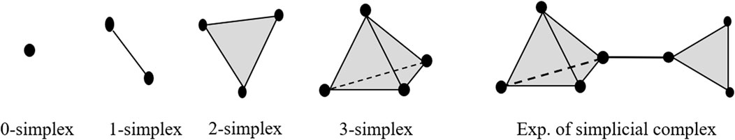
FIGURE 1. k-simplices in ${\mathbb{R}}^3,0\le \mathrm{k}\le 3$ and an example of a simplicial complex.

For a sample X, an interval over the scale ɛ can be found, for which the constructed simplicial complexes belong to the same class of topological invariants as M. By increasing ɛ, a sequence of such complexes will be created, which is called a filtration (Figure 2) with the property:

${\epsilon }_1\le {\epsilon }_2\Rightarrow X\left({\epsilon }_1\right)\subset X\left({\epsilon }_2\right)(3)$

FIGURE 2

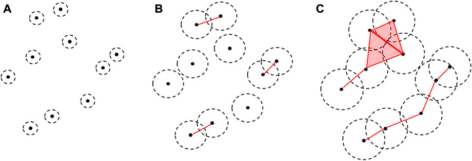
FIGURE 2. Example of filtration varying the filtration value ɛ, which increased from (A–C). The black dot represents the point cloud data connected (red line) when the ɛ-balls around them overlap. The top part of (C) is the union of two adjacent triangles.

During filtration, the classes of n-dimensional topological features -connected components (0-dimension), holes (1-dimension), cavities (2-dimension),…- appear at $b_n^i$ and disappear at $d_n^i$ using the values of ɛ which be computed by persistent homology (Zomorodian and Carlsson, 2005). $b_n^i$ and $d_n^i$ referred to the birth and death values of the i-th class in dimension n, respectively. This information is represented by a collection of points $\left(b_n^i,d_n^i\right)$ drawn in the Cartesian plane ${\mathbb{R}}^2$ and called Persistent Diagram (Figure 3). A persistent diagram is an excellent tool for presenting the robustness and stability of features since the points near the diagonal are often considered noise. In contrast, those further from the diagonal represent more robust topological features.

FIGURE 3

FIGURE 3. The corresponding persistence diagram with H₀(X) in red and H₁(X) in green, representing the persistence of connected components and holes over the ɛ-scale of filtration.

Too few machine learning or statistical tools can be applied directly to persistence diagram space. Hence, a mapping should be done from persistent diagram space to topological vector space, which is appropriate for machine learning tools and further analysis. To achieve this aim by extracting scalar features, there are different methods like persistent image (Adams et al., 2017), persistent landscape (Bubenik, 2015), and persistent entropy (Rucco et al., 2017) methods. Persistent entropy is the (base 2) Shannon entropy of the persistence diagram derived from the filtration. (For simplicity of notation, the log will refer to the log-base-2 function.)

$\mathrm{E}\left(\mathrm{F}\right)=-\sum _1^{\text{n}}{\mathrm{p}}_{\text{i}}\log \left({\mathrm{p}}_{\text{i}}\right),\text{\hspace{0.17em}where\hspace{0.17em}}{\mathrm{p}}_{\text{i}}=\frac{{\mathrm{l}}_{\text{i}}}{{\mathrm{S}}_{\text{L}}},{\mathrm{l}}_{\text{i}}={\mathrm{y}}_{\text{i}}-{\mathrm{x}}_{\text{i}}\text{\hspace{0.17em}and\hspace{0.17em}}{\mathrm{S}}_{\text{L}}=\sum _{\text{i}=1}^{\text{n}}{\mathrm{l}}_{\text{i}}(4)$

3 Related works

There were past attempts to propose cybersickness prediction based on machine learning. The data used can be either based on stereoscopic 3D videos (Padmanaban et al., 2018), profile attributes (Porcino et al., 2020), or physiological signals like electrocardiographic (Garcia-Agundez et al., 2019). In almost all cases, questionnaires were mixed with objective data (Padmanaban et al., 2018), (Porcino et al., 2020), (Garcia-Agundez et al., 2019). Padmanaban et al. (2018) presented a cybersickness prediction algorithm for desktop applications based on a symbolic machine learning model, such as a bagged decision trees classifier (Rao and Potts, 1997) using optical flow as a feature. No physiological signal was recorded during the experiment. Only the combination of two sickness questionnaires: MSSQ and SSQ, was used to find a single sickness value. The precision of their method varied from 26% to 65%, depending on the use case. Some classifiers outperform this (see Section 6).

Porcino et al. (2020), as Padmanaban et al. (2018), presented some classification results without measuring any physiological feedback. Instead, they worked based on profile attributes. They concluded that the most relevant features were the exposure time, the z-axis rotation and profile attributes of the individual (gender, age, and VR experience). Moreover, the VRSQ validated inconsistencies between subjective and objective data captured. As some details, such as the correlation of the features with SSQ, are absent, we could not reproduce their experiment. While very high precision was reported for some classifiers such as Random Forest (96.6% for binary classification of the data from both racing game and flight game scenarios), it is hard to compare and evaluate these results because no physiological feedback was acquired in that experiment.

Porcino et al. (2022) proposed an experimental analysis to estimate the weight of cybersickness causes and not to predict the presence of this phenomenon. These user and context-specific causes were ranked according to their impact using symbolic machine learning in VR games, including a racing game and a flight game. They conducted six experimental protocols along with 37 valid samples from 88 volunteers. They used VRSQ to compare the user discomfort level with the verbal feedback collected during the experiment and thereby evaluated the data and discarded incompatible samples. They achieved 0.79 and 0.95 AUC scores using decision tree and random forest algorithms, respectively. They concluded that exposure time, rotation, and acceleration are likely the top factors contributing to cybersickness. Since this approach, unlike ours, was not to predict the presence of cybersickness, and the input data of their experiment was not based on the participant’s physiological data, it is impossible to compare these results.

The experimental setting of this paper is closer to Garcia et al. (Garcia-Agundez et al., 2019). They collected electrocardiographic, electrooculographic, respiratory, and skin conductivity data from 66 participants given a 10min experiment. They presented two classifiers to classify cybersickness, i.e., Binary and Ternary, based on KNN and SVM classifiers and achieved 82% and 56% accuracy for cybersickness classification, respectively. Some approaches (see Section 6) outperform the ternary classifier. Given the relatively small number of observations, the occasional 82% accuracy of the binary classifier requires investigation with more data. The result of the binary classifier highly depends on several thresholds that need to be selected by the user to define sick people. In our future work, we plan to develop a multi-threshold version of the methods of the present paper.

4 Data measurement and experiment

To collect data and showcase our approach, we performed a user experiment. A total of 53 subjects, 26 females and 27 males, with an age distribution with the mean and the standard deviation of 26.3 years and 3.3 years, respectively, participated in a VR navigation experiment using an HTC Vive Pro head-mounted display. Participants were asked to repeat the experiment three times on 3 days to gather enough samples. In that way, 159 samples were collected and included in the dataset. Upon arrival, participants were asked to sign a consent form and fill out one questionnaire to investigate their health conditions and experience in playing games and using VR devices before participating in the VR task. No issue was reported from this questionnaire. They were then explained the navigation task to achieve, as well as indications on how to navigate using the HTC Vive Pro hand controllers. Participants had to navigate in a virtual forest following a gravel path, including curves and straight lines depicted in Figure 4.

FIGURE 4

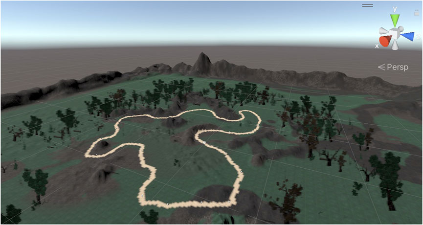
FIGURE 4. Virtual navigation environment used through the experiment. The highlighted line shows the navigation path.

Completing the navigation task took approximately 4 minutes. A Simulator Sickness Questionnaire (SSQ) was deployed in the experiment in which three different categories (nausea, oculomotor, disorientation) were measured in the form of 16 questions to quantify the severity of each possible symptom of cybersickness. Participants filled one SSQ before and after the experiment to measure the psychological impact of the VR task on them. The difference between the pre-exposure and the post-exposure scores (called SSQ score) was included in the dataset:

$\mathrm{S}\mathrm{S}\mathrm{Q}=SS{Q}_{\text{post\hspace{0.17em}}}-{\mathrm{S}\mathrm{S}\mathrm{Q}}_{\text{pre\hspace{0.17em}}}(5)$

It is worth noting that we used the SSQ as a subjective tool, as being very predominant and largely administered in most VR studies, despite the existence of strong debates about its validity and reliability in VR studies [e.g., (Sevinc and Berkman, 2020) or (Bouchard et al., 2021)] and recommendation to use VR-more-dedicated questionnaires, such as the VRSQ. This paper focuses on a methodology to grasp and predict cybersickness from any sickness-related data; we leave the use of different subjective means and their incidence on our method for future work.

An Empatica E4 wristband¹ on one participant’s arm was used for real-time physiological data acquisition, particularly the participants’ electrodermal activity (EDA) during this experiment. This wearable device is equipped with sensors to gather high-quality data sent during navigation to a processing computer through Bluetooth. These sensors have different frequencies for measurement data sampling: EDA sensor 4 Hz, PPG Sensor 64 Hz (BVP), Infrared Thermopile 4Hz (TEM), 3-axis accelerometer sensor 32Hz, and average heart rate values are computed in spans of 10 seconds. Galvanic Skin Response (GSR), blood volume pressure (BVP), heart rate (HR), and temperature (TEM) were recorded during their navigation experiment. Moreover, the recorded navigation speed computed the longitudinal (LG) and rotational (RT) accelerations. An example of the recorded signals is shown in Figure 5.

FIGURE 5

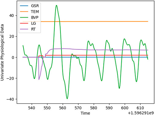
FIGURE 5. Sample of multivariate physiological data.

5 Methodology and implementation

We propose an overall workflow in four steps for the complete detection process, as shown in Figure 6. The workflow represented in this Figure has two main sub-processes: pre-processing, data structure analysis, labelling of the data (steps 1–3), and classification (step 4).

FIGURE 6

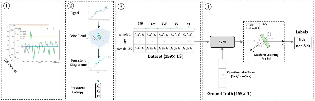
FIGURE 6. Block diagram of the cybersickness prediction method. 1) Normalization of the time series as a pre-processing step 2) Applying TDA and vectorizing persistent diagram to persistent entropy 3) Making the dataset (159 × 15 matrix) from the features descriptors that characterize the sample’s data 4) Feeding the dataset into the SVM classifier along with ground truth labels (i.e., sick:1 and non-sick:0) provided by the questionnaire scores. Finally, SVM finds a suitable hyperplane (the green surface shown in the Figure) that can cleanly separate the samples into two groups (i.e., sick and non-sick). The method’s output is a set of predicted labels based on the decision made by the SVM classifier.

Recorded data for each subject includes five sensor output variables, as discussed in the previous section. Each variable corresponds to one physiological sensor data. Applying the persistent entropy, three features are obtained per each variable: birth, death, and dimension. We obtain the dataset with 159 rows and 5 × 3 = 15 columns, where each row is related to each sample.

As data recording was performed with different frequencies, discussed in Section 4, the timesteps of various time series differed. Therefore, as the first pre-processing step, we normalized the data based on minimum timesteps throughout the dataset.

We improved our pre-processing in the workflow by adding a denoising approach. We applied Empirical Mode Decomposition (EMD) to the physiological data on every variable before applying the TDA. EMD is used to decompose the time series into a finite and often small number of components named its Intrinsic Mode Functions (IMFs) and residue series (Pereira and de Mello, 2015). To decompose a signal and get the IMFs, lower and upper envelopes are obtained by connecting all the local maxima/minima using a cubic spline. Subsequently, a low-frequency component is calculated using the mean of these envelopes. This component is subtracted from the original signal. Eventually, based on two specific criteria detailed in (Huang et al., 1998), the output signal is calculated as an IMF.

EMD determines what frequency with what strength in the signal occurs at any given moment. IMFs can be summed to recover the original signal. Because the first IMF usually carries the most oscillating (high-frequency) components, it can be rejected to remove high-frequency components (e.g., random noise). Figure 7 shows one example of EMD applied to the GSR time series. Original, decomposed, and reconstructed signals are shown on the left, middle and right sides.

FIGURE 7

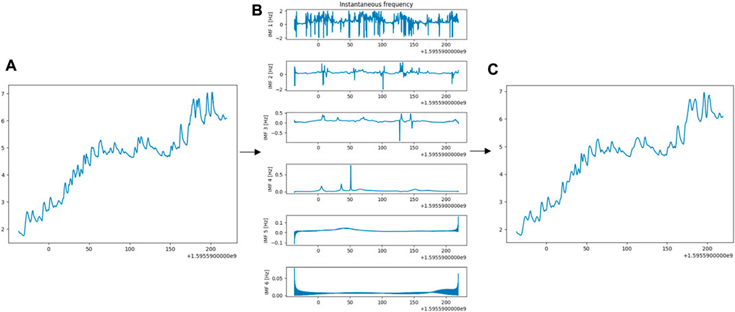
FIGURE 7. (A) Original GSR time series (B) Six IMFs decomposed by EMD (C) Output Series from EMD on the original signal. It is the sum of the last five IMFs plus residue.

After pre-processing, we additionally do qualitative data structure analysis. We detected the 0 (connected components), 1 (loop), and 2 (void) dimensional persistent topological features across multiple scales. We used the time delay embedding method, based on the results of Taken’s embedding theorem (Takens, 1981), which can be considered sliding a specific size wind over the signal. Each window is represented as a point in a high-dimensional space.

More formally, given a time series f(t), a sequence of vectors extracted has the form:

${\mathrm{f}}_{\text{i}}=\left[\mathrm{f}\left({\mathrm{t}}_{\text{i}}\right),\mathrm{f}\left({\mathrm{t}}_{\text{i}}+2\tau \right),\dots ,\mathrm{f}\left({\mathrm{t}}_{\text{i}}+\left(\mathrm{M}-1\right)\tau \right)\right]\in {\mathbb{R}}^{\text{d}}(6)$

Where (M-1) is the embedding dimension and τ is the time delay. Hence, the window size is the quantity (M-1)τ and a stride is defined as the difference between t_i and t_i+1. In other words, the time delay embedding of f with parameters (M,τ) is the function:

${\mathrm{T}\mathrm{D}}_{\text{M},\tau }\mathrm{f}:\mathbb{R}\to {\mathbb{R}}^d,\mathrm{t}\to \left[\begin{array}{c}\hfill \mathrm{f}\left(\mathrm{t}\right)\hfill \\ \hfill \mathrm{f}\left(\mathrm{t}+\tau \right)\hfill \\ \hfill \mathrm{f}\left(\mathrm{t}+2\tau \right)\hfill \\ \hfill \cdots \hfill \\ \hfill \mathrm{f}\left(\mathrm{t}+\left(\mathrm{M}-1\right)\tau \right)\hfill \end{array}\right](7)$

As a result, we have two hyperparameters: M,τ. To determine the time delay automatically, we used the Mutual Information (MI) technique (Wen and Wan, 2009). MI is used as an analytical measure of the extent to which earlier values can predict the values in the time series. At first, the time series’ Probability Density Function (PDF) is calculated with n bins. Given p_i as the probability that x_t is in the i^th bin (marginal probability density distribution) and p_i,j as the probability that x_t is in the j^th bin while x_t+τ is in the i^th bin (joint probability density distribution), MI is defined as Kulback-Liebler (KL) divergence between the p_i,j and p_i and p_j i.e.

$I\left(\tau \right)=-\sum _{i=1}^{n_{\text{bins\hspace{0.17em}}}}\sum _{j=1}^{n_{\text{bins\hspace{0.17em}}}}{p}_{i,j}\left(\tau \right)\log \frac{p_{i,j}\left(\tau \right)}{p_i{p}_j}(8)$

According to the MI technique, the optimal time delay can be computed as the minimum value of I(τ).

The False Nearest Neighbor (FNN) technique is used to get the optimal value for embedding dimension M. According to this algorithm, points lying close together due to projection are separated in higher embedding dimensions. Conversely, nearest neighbour points which are close in one embedding dimension should be close in a higher one. Suppose that p_j is the nearest neighbour of p_i in m-dimensional space. The Euclidean distance between p_i and p_j is:

$R_m^2\left(i,j\right)=\sum _{k=0}^{m-1}{\left[x\left(i+k\tau \right)-x\left(j+k\tau \right)\right]}^2(9)$

By adding one more dimension, the distance will change:

$R_{m+1}^2\left(i,j\right)=R_m^2\left(i,j\right)+{\left[x\left(i+m\tau \right)-x\left(j+m\tau \right)\right]}^2(10)$

Then, the FNN criterion is defined as:

$R_i={\left(\frac{R_{m+1}^2\left(i,j\right)-R_m^2\left(i,j\right)}{R_m^2\left(i,j\right)}\right)}^{\frac{1}{2}}=\frac{|x\left(i+m\tau \right)-x\left(j+m\tau \right)|}{R_d\left(i,j\right)}>R_{th}(11)$

More formally, if we have a point p_i and neighbour p_j, we check if the normalized distance R_i for the next dimension is more significant than some threshold R_th. If R_i > R_th, we have a false nearest neighbour, and the optimal embedding dimension is obtained by minimizing the total number of such neighbours.

In a nutshell, time delay embeddings translate a 1-dimensional time series to a d-dimensional time series in which the current value at each time with (d − 1) lags.

After the data structure analysis, the physiological data were labelled using the participants’ self-reported sickness questionnaire collected during the VR experiment. To achieve this aim, the SSQ score was collected pre- and post-exposure, and the score for each participant was calculated using original indexes (see Section 4). We considered the SSQ score of 20 as the threshold to define the label of “sick” and “non-sick” (Bimberg et al., 2020). The participants whose SSQ score is equal to or greater than 20 are assumed to suffer from cybersickness and “sick”. Conversely, an SSQ score of less than 20 is defined as not experiencing cybersickness and labelled “non-sick”. This step leads to a data size table 159 × 15, as shown in Figure 6. Based on this labelling, the 159 samples were divided into 87 and 72 “sick” and “non-sick” samples.

The next step of the workflow is the classification of the data. This includes selecting a good classifier, training the classifier with the above data, and evaluating the classifier’s performance on some test data. The data extracted in step 3 is used as an input to the machine learning classifier with two classes, i.e., “sick” and “non-sick”.

To investigate the effect of the machine learning classification algorithms on the performance and accuracy of the detection process, we selected several classifiers of different types and implemented them in the workflow. First, we applied SVM classifiers with linear, polynomial (second degree) and Gaussian RBF (gamma = 10^–5, C = 1, regularization parameter = 1) kernels. Second, we used Random Forest as an ensemble method considering two features when looking for the best split, 100 Decision Trees in the forest, Gini as the criteria with which to split on each node, minimum of two samples to split an internal node, and minimum 1 sample to be at a leaf node. As the last classifier algorithm, Logistic Regression with “lbfgs” as the solver used for the optimization problem, a maximum of 500 iterations was taken to converge the solvers, “l2” as the penalty, and C = 1 to control the penalty strength was compared. In total, five classifiers were implemented and tested.

After applying EMD, we investigated the TDA performance on raw and denoised signal reconstructed, summing the last five IMFs plus residue. Additional classification algorithms that were implemented and compared to TDA were the bag-of-patterns (Lin et al., 2012)with sliding window size 16, length of the words 4, and 4 bins to produce without numerosity reduction; ROCKET (Dempster et al., 2020) with 10000 kernels in sizes 7,9, and 11; WEASEL (Schäfer and Leser, 2017) with word size 9 and window sizes from 10 to 27. In all mentioned studies, SVM (Gaussian RBF) with the parameters mentioned above was used as the classifier.

Another point that we have investigated was which kind of physiological data has more influence on cybersickness prediction. We applied the compound approach of TDA with SVM (Gaussian RBF) to different combinations of variables. The performance and accuracy of each classifier were evaluated using the F1 score metric because we had an imbalanced classification problem.

${\mathrm{F}}^1=\left(\frac{2}{{\text{\hspace{0.17em}recall\hspace{0.17em}}}^{-1}+{\text{\hspace{0.17em}precision\hspace{0.17em}}}^{-1}}\right)=2.\frac{\text{\hspace{0.17em}precision\hspace{0.17em}}\ast \text{\hspace{0.17em}recall\hspace{0.17em}}}{\text{\hspace{0.17em}precision\hspace{0.17em}}+\text{\hspace{0.17em}recall\hspace{0.17em}}}(12)$

$\text{\hspace{0.17em}precision\hspace{0.17em}}=\frac{\mathrm{T}\mathrm{P}}{\mathrm{T}\mathrm{P}+\mathrm{F}\mathrm{P}},\text{\hspace{0.17em}recall\hspace{0.17em}}=\frac{\mathrm{T}\mathrm{P}}{\mathrm{T}\mathrm{P}+\mathrm{F}\mathrm{N}}(13)$

To assess the generalization ability of the classifier and evaluate and test its performance, we used K-fold Cross-Validation (CV) technique (Berrar, 2019) with K = 5. Also, we computed the evaluation metric, i.e., the F1 score and its mean and standard deviation (std) in every fold. Finally, we summarized the model’s efficiency using the averaging of model evaluation scores as demonstrated in Figure 8.

FIGURE 8

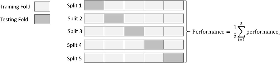
FIGURE 8. 5-Fold cross-validation in which data is divided into 5-folds composed of 4-folds for training the model and 1-fold for validation. The overall performance is obtained by computing the arithmetic mean.

6 Results and discussion

As discussed in Section 5, first, we have presented the pre-processing, the TDA-based feature descriptor (in three steps) and machine learning classifiers to classify sensor data into two classes. Then, we analyzed the accuracy of TDA in combination with various classification algorithms. In the second investigation, we applied other types of feature descriptors dedicated to tackling time series classification and compared the results with TDA. In the third investigation, we studied the effect of the heat rate signal on the classification.

6.1 Comparison of classification algorithms

The effect of the classification algorithm on the correct detection of the affected subjects is demonstrated in Table 1. Figure 9 visually demonstrates these outcomes. As seen, the SVM (Gaussian RBF) presents a higher mean and lower standard deviation (std) than other classifiers in the F1 score metric, which means a more accurate and more stable classification, with around 71% of accuracy. Interestingly, while the mean of the F1 metric decreases from SVM (Gaussian RBF) to SVM (linear kernel) in Table 1, the standard deviation (std) consistently increases conversely. The worst classification result was achieved by SVM (linear kernel), with an average precision of 61%.

TABLE 1

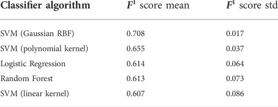
TABLE 1. Comparison between various classification algorithms in combination with TDA.

FIGURE 9

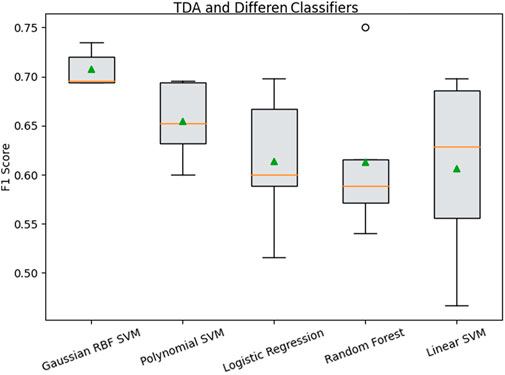
FIGURE 9. Performance evaluation and the effect of the classifier on sickness detection using the TDA feature descriptor.

Our explanation for this performance is that Gaussian RBF kernels provide embeddings of physiological time series data into spaces rich enough to capture the essential geometric features of these time series. Therefore, we consider SVM (with Gaussian RBF) the more robust classifier algorithm for this data type. We will be using it below to analyze the effect of feature descriptors on cybersickness detection.

6.2 Comparison of compound classifiers

Five feature descriptors were selected: TDA, EMD + TDA, bag-of-patterns, ROCKET, and WEASEL, and applied to the data to extract features. The features were classified using SVM (Gaussian RBF) with the configuration detailed in Section 5. The mean and the standard deviation of the F1 score are presented in Table 2 and visualized similar to the classifier effect as shown in Figure 10. The first finding is that the ROCKET feature descriptor achieved a little better precision, 71%, a higher mean F1 score and less standard deviation (std) than TDA. However, the difference in the F1 score is only 0.002, with a 0.001 difference in standard deviation, on the dataset of 159 time series, which indicates that the difference between ROCKET and TDA is not statistically significant.

TABLE 2

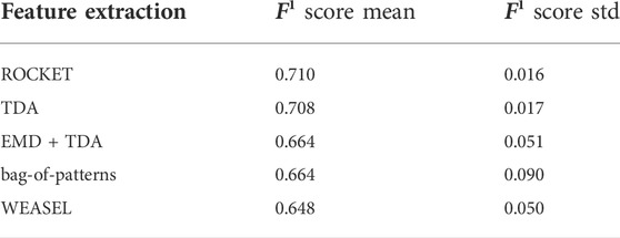
TABLE 2. Comparison between TDA and four other methods and their effect on performance.

FIGURE 10

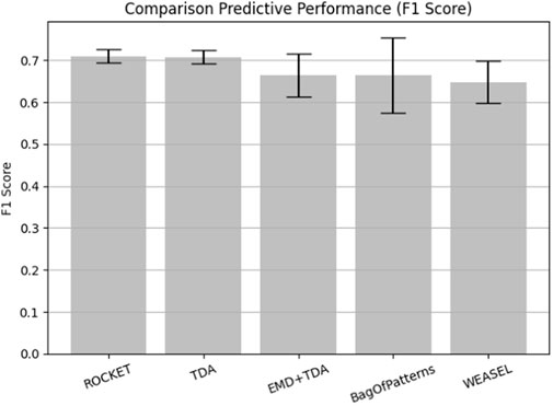
FIGURE 10. Performance evaluation using different feature extraction algorithms.

As ROCKET uses a very large number of random convolutional kernels (10000 in this case), it is a more computationally demanding method than the TDA. Due to the technical similarities with convolutional neural networks, we expect that a rigorous mathematical or statistical performance analysis and explicit interpretation of solutions would be difficult for ROCKET. On the other hand, given that TDA is based on basic concepts of mathematical topology and that SVMs are already proven to be universally consistent, combinations of TDA and SVMs are expected to be much easier for both rigorous analyses for explainability.

It turned out that the mean of the evaluated metric of the TDA alone is higher than that of a more complex combination of TDA with EMD denoising and conversely, its standard deviation (std) is less. This implies that important details of the sensor data are removed by EMD during the denoising process. It can be concluded the EMD parameter shall be set more precisely taking into account the sampling frequency of each signal otherwise some useful high-frequency information, where they are close to the noise, can be easily eliminated with the improper setting of filtering parameters. A mathematical framework accounting for this effect was developed in (Langovoy, 2007). In all other cases, TDA has a higher mean F1 score and a smaller standard deviation (std).

6.3 Heart rate and cybersickness

The result of the third investigation is shown in Table 3. Including the heart rate features leads to lower precision, high stability, and a significant standard deviation (std) increase. Therefore, this sensor data was excluded from the above analysis. Surprisingly, heart rate was not a relevant predictor for cybersickness. Since the heart rate sampling is less than the other signals, a large portion of the signals and, subsequently, the details are removed during the normalization phase, leading to a decrease in prediction accuracy.

TABLE 3

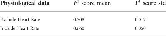
TABLE 3. The effect of heart rate (HR) on cybersickness prediction.

7 Conclusion

In this paper, we proposed a machine learning approach to VR’s cybersickness prediction based on physiological and subjective data. We investigated dynamic topological data analysis combinations with a range of classifier algorithms and assessed classification performance using the F1 score.

The highest performance of TDA-based methods was achieved in combination with an SVM with a Gaussian RBF kernel. Our explanation for this performance is that Gaussian RBF kernels provide embeddings of physiological time series data into spaces rich enough to capture the essential geometric features of these time series.

A comparison of TDA with other feature descriptors for physiological time series classification showed that the performance of TDA + SVM is at the top of the list: whilst it is slightly lower than ROCKET + SVM, the difference is not significant, and the accuracy is higher than combinations of SVMs with bag-of-patterns and WEASEL.

As ROCKET uses a very large number of random convolutional kernels (10000 in this case), it is a more computationally demanding method than the TDA. Due to the technical similarities with convolutional neural networks, we expect that a rigorous mathematical or statistical performance analysis and explicit interpretation of solutions would be difficult for ROCKET. On the other hand, given that TDA is based on basic concepts of mathematical topology and that SVMs are already proven to be universally consistent, combinations of TDA and SVMs are expected to be much easier for both rigorous analyses for explainability. Similar reasoning can be applied to complex methods such as bag-of-patterns and WEASEL.

We noticed that performance of TDA-based methods on time series data got worse after adding the standard EMD reconstruction. This warns against the noncritical application of data smoothing and data transformation techniques.

Surprisingly, our results show that heart rate does not affect cybersickness prediction. It remains to investigate whether this would be the case for other VR experiments.

In addition, a few machine learning or statistical tools can be applied directly to the persistence diagram space. We will attempt to create such machine learning tools by proposing visual perception-based metrics for persistence diagram spaces, similar to. This will allow more direct and advanced combinations of machine learning methods with the TDA.

Data availability statement

The original contributions presented in the study are included in the article/supplementary materials, further inquiries can be directed to the corresponding author.

Ethics statement

Ethical review and approval was not required for the study on human participants in accordance with the local legislation and institutional requirements. The patients/participants provided their written informed consent to participate in this study.

Author contributions

AH, CG, JC, ML and JO contributed to conception and design of the study. YW organized the database. AH performed the statistical analysis. AH wrote the first draft of the manuscript. CG, JC, and ML wrote sections of the manuscript. All authors contributed to manuscript revision, read, and approved the submitted version.

Funding

This work was supported in part by a grant from the French-German University (UFA-DFH) No. CDFA 03–19.

Conflict of interest

The authors declare that the research was conducted in the absence of any commercial or financial relationships that could be construed as a potential conflict of interest.

The remaining authors declare that the research was conducted in the absence of any commercial or financial relationships that could be construed as a potential conflict of interest.

Publisher’s note

All claims expressed in this article are solely those of the authors and do not necessarily represent those of their affiliated organizations, or those of the publisher, the editors and the reviewers. Any product that may be evaluated in this article, or claim that may be made by its manufacturer, is not guaranteed or endorsed by the publisher.

Footnotes

¹https://www.empatica.com/research/e4/.

References

Adams, H., Emerson, T., Kirby, M., Neville, R., Peterson, C., Shipman, P., et al. (2017). Persistence images: A stable vector representation of persistent homology. J. Mach. Learn. Res. 18.

Google Scholar

Berrar, D. (2019). Cross-validation.

Google Scholar

Bimberg, P., Weissker, T., and Kulik, A. (2020). “On the usage of the simulator sickness questionnaire for virtual reality research,” in 2020 IEEE conference on virtual reality and 3D user interfaces abstracts and workshops, 464–467.

CrossRef Full Text | Google Scholar

Bouchard, S., Berthiaume, M., Robillard, G., Forget, H., Daudelin-Peltier, C., Renaud, P., et al. (2021). Arguing in favor of revising the simulator sickness questionnaire factor structure when assessing side effects induced by immersions in virtual reality. Front. Psychiatry 12, 739742. doi:10.3389/fpsyt.2021.739742

PubMed Abstract | CrossRef Full Text | Google Scholar

Bubenik, P. (2015). Statistical topological data analysis using persistence landscapes. J. Mach. Learn. Res. 16, 77–102.

Google Scholar

Carlsson, G. (2009). Topology and data. Bull. Amer. Math. Soc. 46, 255–308. doi:10.1090/s0273-0979-09-01249-x

CrossRef Full Text | Google Scholar

Chardonnet, J.-R., Mirzaei, M. A., and Mérienne, F. (2017). Features of the postural sway signal as indicators to estimate and predict visually induced motion sickness in virtual reality. Int. J. Human–Computer. Interact. 33, 771–785. doi:10.1080/10447318.2017.1286767

CrossRef Full Text | Google Scholar

Chardonnet, J.-R., Mirzaei, M. A., and Merienne, F. (2021). Influence of navigation parameters on cybersickness in virtual reality. Virtual Real. 25, 565–574. doi:10.1007/s10055-020-00474-2

CrossRef Full Text | Google Scholar

Dempster, A., Petitjean, F., and Webb, G. I. (2020). Rocket: Exceptionally fast and accurate time series classification using random convolutional kernels. Data Min. Knowl. Discov. 34, 1454–1495. doi:10.1007/s10618-020-00701-z

CrossRef Full Text | Google Scholar

Diersch, N., and Wolbers, T. (2019). The potential of virtual reality for spatial navigation research across the adult lifespan. J. Exp. Biol. 222, jeb187252. doi:10.1242/jeb.187252

PubMed Abstract | CrossRef Full Text | Google Scholar

Frank, L., Kennedy, R. S., Kellogg, R. S., and McCauley, M. E. (1983). Simulator sickness: A reaction to a transformed perceptual world. Tech. rep. EOTR 88-2. Orlando, FL: ESSEX CORP.

Google Scholar

Garcia-Agundez, A., Reuter, C., Becker, H., Konrad, R., Caserman, P., Miede, A., et al. (2019). Development of a classifier to determine factors causing cybersickness in virtual reality environments. Games health J. 8, 439–444. doi:10.1089/g4h.2019.0045

PubMed Abstract | CrossRef Full Text | Google Scholar

Hatcher, A. (2002). Algebraic topology, Cambridge University Press.

Google Scholar

Hausmann, J.-C. (1995). On the vietoris-rips complexes and a cohomology theory for metric spaces. Ann. Math. Stud. 138, 175–188.

Google Scholar

Huang, N. E., Shen, Z., Long, S. R., Wu, M. C., Shih, H. H., Zheng, Q., et al. (1998). The empirical mode decomposition and the hilbert spectrum for nonlinear and non-stationary time series analysis. Proc. R. Soc. Lond. A 454, 903–995. doi:10.1098/rspa.1998.0193

CrossRef Full Text | Google Scholar

Jeong, D., Yoo, S., and Yun, J. (2019). “Cybersickness analysis with eeg using deep learning algorithms,” in IEEE conference on virtual reality and 3D user interfaces. 827–835.

CrossRef Full Text | Google Scholar

Kennedy, R. S., Lane, N. E., Berbaum, K. S., and Lilienthal, M. G. (1993). Simulator sickness questionnaire: An enhanced method for quantifying simulator sickness. Int. J. Aviat. Psychol. 3, 203–220. doi:10.1207/s15327108ijap0303_3

CrossRef Full Text | Google Scholar

Keshavarz, B., and Hecht, H. (2011). Validating an efficient method to quantify motion sickness. Hum. Factors 53, 415–426. doi:10.1177/0018720811403736

PubMed Abstract | CrossRef Full Text | Google Scholar

Kim, H. K., Park, J., Choi, Y., and Choe, M. (2018). Virtual reality sickness questionnaire (vrsq): Motion sickness measurement index in a virtual reality environment. Appl. Ergon. 69, 66–73. doi:10.1016/j.apergo.2017.12.016

PubMed Abstract | CrossRef Full Text | Google Scholar

Kim, J., Kim, W., Oh, H., Lee, S., and Lee, S. (2019). “A deep cybersickness predictor based on brain signal analysis for virtual reality contents,” in Proceedings of the IEEE/CVF International Conference on Computer Vision, Seoul, Korea (South), October 2019 - 02 November 2019, 10580.

CrossRef Full Text | Google Scholar

Langovoy, M. (2007). Data-driven goodness-of-fit tests. arXiv preprint arXiv:0708.0169.

Google Scholar

Lee, S., Kim, S., Kim, H. G., Kim, M. S., Yun, S., Jeong, B., et al. (2019). “Physiological fusion net: Quantifying individual vr sickness with content stimulus and physiological response,” in IEEE international conference on image processing (ICIP). IEEE, 440–444.

CrossRef Full Text | Google Scholar

Liao, C.-Y., Tai, S.-K., Chen, R.-C., and Hendry, H. (2020). Using eeg and deep learning to predict motion sickness under wearing a virtual reality device. IEEE Access 8, 126784–126796. doi:10.1109/access.2020.3008165

CrossRef Full Text | Google Scholar

Lin, C.-T., Tsai, S.-F., and Ko, L.-W. (2013). Eeg-based learning system for online motion sickness level estimation in a dynamic vehicle environment. IEEE Trans. Neural Netw. Learn. Syst. 24, 1689–1700. doi:10.1109/tnnls.2013.2275003

PubMed Abstract | CrossRef Full Text | Google Scholar

Lin, J., Khade, R., and Li, Y. (2012). Rotation-invariant similarity in time series using bag-of-patterns representation. J. Intell. Inf. Syst. 39, 287–315. doi:10.1007/s10844-012-0196-5

CrossRef Full Text | Google Scholar

Mazloumi Gavgani, A., Walker, F. R., Hodgson, D. M., and Nalivaiko, E. (2018). A comparative study of cybersickness during exposure to virtual reality and “classic” motion sickness: Are they different? J. Appl. Physiology 125, 1670–1680. doi:10.1152/japplphysiol.00338.2018

CrossRef Full Text | Google Scholar

Merienne, F. (2017). Virtual reality: Principles and applications. In Encyclopedia of Computer Science and Technology. Taylor & Francis.

CrossRef Full Text | Google Scholar

Moroni, D., and Pascali, M. A. (2021). Learning topology: Bridging computational topology and machine learning. Pattern Recognit. Image Anal. 31, 443–453. doi:10.1134/s1054661821030184

CrossRef Full Text | Google Scholar

Niu, Y., Wang, D., Wang, Z., Sun, F., Yue, K., and Zheng, N. (2020). User experience evaluation in virtual reality based on subjective feelings and physiological signals. Electron. Imaging 2020, 60413–60421.

Google Scholar

Padmanaban, N., Ruban, T., Sitzmann, V., Norcia, A. M., and Wetzstein, G. (2018). Towards a machine-learning approach for sickness prediction in 360 stereoscopic videos. IEEE Trans. Vis. Comput. Graph. 24, 1594–1603. doi:10.1109/tvcg.2018.2793560

PubMed Abstract | CrossRef Full Text | Google Scholar

Pereira, C. M., and de Mello, R. F. (2015). Persistent homology for time series and spatial data clustering. Expert Syst. Appl. 42, 6026–6038. doi:10.1016/j.eswa.2015.04.010

CrossRef Full Text | Google Scholar

Pincus, S. M., and Goldberger, A. L. (1994). Physiological time-series analysis: What does regularity quantify? Am. J. Physiology-Heart Circulatory Physiology 266, H1643–H1656. doi:10.1152/ajpheart.1994.266.4.h1643

PubMed Abstract | CrossRef Full Text | Google Scholar

Plouzeau, J., Chardonnet, J.-R., and Merienne, F. (2018). Using cybersickness indicators to adapt navigation in virtual reality: A pre-study. in IEEE conference on virtual reality and 3D user interfaces. 661–662.

CrossRef Full Text | Google Scholar

Porcino, T., Rodrigues, E. O., Bernardini, F., Trevisan, D., and Clua, E. (2022). Identifying cybersickness causes in virtual reality games using symbolic machine learning algorithms. Entertain. Comput. 41, 100473. doi:10.1016/j.entcom.2021.100473

CrossRef Full Text | Google Scholar

Porcino, T., Rodrigues, E. O., Silva, A., Clua, E., and Trevisan, D. (2020). “Using the gameplay and user data to predict and identify causes of cybersickness manifestation in virtual reality games,” in 2020 IEEE 8th international conference on serious games and applications for health. 1–8.(SeGAH) (IEEE).

CrossRef Full Text | Google Scholar

Rao, J. S., and Potts, W. J. (1997). Visualizing bagged decision trees. KDD, 243–246.

Google Scholar

Rucco, M., Gonzalez-Diaz, R., Jimenez, M.-J., Atienza, N., Cristalli, C., Concettoni, E., et al. (2017). A new topological entropy-based approach for measuring similarities among piecewise linear functions. Signal Process. 134, 130–138. doi:10.1016/j.sigpro.2016.12.006

CrossRef Full Text | Google Scholar

Schäfer, P., and Leser, U. (2017). Fast and accurate time series classification with weasel. Proc. 2017 ACM Conf. Inf. Knowl. Manag., 637–646.

Google Scholar

Schölkopf, B., and Smola, A. J. (2018). Learning with kernels: Support vector machines, regularization, optimization, and beyond. MIT press.

Google Scholar

Sevinc, V., and Berkman, M. I. (2020). Psychometric evaluation of simulator sickness questionnaire and its variants as a measure of cybersickness in consumer virtual environments. Appl. Ergon. 82, 102958. doi:10.1016/j.apergo.2019.102958

PubMed Abstract | CrossRef Full Text | Google Scholar

Strang, G. (2006). Linear algebra and its applications. Belmont, CA: Thomson, Brooks/Cole.

Google Scholar

Takens, F. (1981). “Detecting strange attractors in turbulence,” in Dynamical systems and turbulence, Warwick 1980. Lecture notes in mathematics. Editors D. Rand, and L. S. Young (Berlin, Heidelberg: Springer), 898 doi:10.1007/BFb0091924

CrossRef Full Text | Google Scholar

Wen, F., and Wan, Q. (2009). “Time delay estimation based on mutual information estimation,” in 2nd International Congress on Image and Signal Processing, 1–5.

Google Scholar

West, D. B. (2001). Introduction to graph theory. Pearson College Div.

Google Scholar

Zomorodian, A., and Carlsson, G. (2005). Computing persistent homology. Discrete Comput. Geom. 33, 249–274. doi:10.1007/s00454-004-1146-y

CrossRef Full Text | Google Scholar