Towards Real-Time 3D Editable Model Generation for Existing Indoor Building Environments on a Tablet

This paper describes a mobile application that builds and updates a 3D model of an indoor environment, including walls, floor and openings, by a simple scan performed using a tablet equipped with a depth sensor. This algorithm is fully implemented on the device, does not require internet connection and runs in real-time, i.e., at five frames per second. This is made possible by taking advantage of recent AR frameworks, by assuming that the structure of the room is aligned on an Euclidean grid and by simply starting the scan in front of a wall. The wall detection is achieved in two steps. First, each incoming point cloud is segmented into planar wall candidates. Then, these planes are matched to the previously detected planes and labeled as ground, ceiling, wall, openings or noise depending on their geometric characteristics. Our evaluations show that the algorithm is able to measure a plane-to-plane distance with a mean error under 2 cm, leading to an accurate estimation of a room dimensions. By avoiding the generation of an intermediate 3D model, as a mesh, our algorithm allows a significant performance gain. The 3D model can be exported to a CAD software, in order to plan renovation works or to estimate energetic performances of the rooms. In the user experiments, a good usability score of 75 is obtained.

1 Introduction

Creating a 3D model of an existing building has found many applications, such as the generation of a BIM¹ of the building or obtaining geometrical information about the building (dimensions, surfaces, etc.,). Whereas a 3D model of a new building is created during the conception phase, older buildings have frequently to be modeled. This process is often done manually for smaller buildings and is very tedious. For large scale buildings, laser scanners are used to generate high resolution 3D point clouds. These laser data serve as a basis to identify the structure of the reconstructed building. In addition, the process for exporting a BIM model can be partially automated (Macher et al., 2015).

However performing an automatic generation of a 3D editable model of buildings is a complex task. Most of the previous works have focused on recognizing the global structure (grounds, ceiling, walls and openings) of the reconstructed building. Moreover, the use of laser scanners and LIDAR is costly and the scan is not performed in real time.

When only a rough global structure of the building is needed, or when the housing is small, it is possible to simplify the process.

With the recent release of depth sensors integrated onto tablets and with the enhancement of their computing capabilities, it is now possible to use these devices to perform a real-time 3D reconstruction. This can be bought at an affordable price by companies or by private individuals who want to renovate their housings. The measure of each dimension of the room and the edition in a CAD software, are very time expensive tasks, that can be made easier by the simple scan, as proposed in this paper.

This paper presents an application that allows any user to generate a 3D editable model of an existing indoor environment using a tablet or a smartphone, by simply walking inside the building and scanning the walls. The resulting model can then be exported in a CAD² software for modification, for renovation or decorating purposes and for estimating the energetic performances. The device has to include a visual odometry system, which is the case with modern AR APIs such as Google ARCore³, so that each RGB-D data issued from the sensors can be expressed in a same absolute coordinates frame. The proposed algorithm uses the computing capabilities of the device to generate a 3D editable model on-the-fly, including the walls and openings of the rooms. Thus, it avoids the generation of an intermediate 3D mesh, which is costly in terms of memory and computing resources Arnaud et al. (2016). A RGB-D sensor is used, which provides a temporal sequence of color and depth data captured at five frame per second. First, a planar segmentation is performed in each depth image of the sequence and the extracted planes are matched to the previously detected ones. Through this temporal analysis, walls are extracted and described in terms of geometry and, the global 3D model is updated.

The proposed algorithm assumes that the walls, the ceiling, and the floor are aligned on a Euclidean grid, which is a common assumption when working with building data Coughlan and Yuille (1999). It also assumes that the scan starts in front of a wall. These reasonable assumptions lead to considerable simplifications of the reconstruction process.

The previous work Arnaud et al. (2018) was a first attempt of real-time planes detection and matching using a mobile device, and was dedicated to the segmentation method. Color, luminance edges and point cloud were analyzed together through a bottom-up segmentation process, which combined a region growing method with a merging. Although the process was real-time (the data was processed in approximately 200 ms), some experiments have shown that, in some situations, only 40% of the planar surfaces were correctly detected. The present paper details each component of the application, from the extraction of 3D planes to their export towards a CAD software. Concerning the 3D scanning and modeling, which is the most time-consuming task of the application, a top-down hierarchical segmentation is achieved directly on the point cloud, without any pre-processing. A first stage is dedicated to the detection of rough planar categories, which are then separated into parallel planes. By capturing the most dominant planes, the method proves less sensitive to noise than the top-down strategy. In addition, the multi-threading is made possible by an adapted tree sorting of the points. The planar surfaces that are extracted in two successive frames are matched temporally, then walls and openings are identified. To finish, this paper explains the different components of a more comprehensive mobile application, which is able to create and export a 3D model that can be used and edited in a CAD software, to plan renovation works and to estimate energetic performance.

In the rest of this paper, some previous works on 3D segmentation and classification are described (Section 2). Then, the planar segmentation algorithm is developed in Section 3 while the temporal matching and the model export are detailed in Section 4. The results of the evaluations conducted for these algorithms are presented in Section 5 and discussed.

2 Related Works

3D modeling of indoor environments has been the subject of numerous research studies, as noticed by the recent review Kang et al. (2020). One of the strategies consists in capturing and mapping a dense colored point cloud Henry et al. (2012) into a real coordinate system, in which it is possible to navigate virtually. From depth data, a 3D mesh of the whole scene can first be estimated, and eventually simplified Liang et al. (2020). Since our main objective is to propose a stand-alone 3D modeling application for mobile devices, such as tablets or smartphones, such dense models are not optimal since they require a large amount of memory resources. In addition, we intend to produce a 3D model in real-time, without connecting to a distance webservice. Indeed, internet connection is not available on all worksites. Since the sensor captures one point cloud each 200 ms, it is necessary to compute a 3D model in this period of time, otherwise the next point cloud can be lost. For that purpose, 3D segmentation techniques are promising (Section 2.1). From the point cloud, these techniques directly detect planar structures from the point cloud and convert them into parameterized shapes (for example by simply storing the coordinates of their four corners). All the surfaces can be locally viewed as planar surfaces Tatavarti et al. (2017) that can be further analyzed using classification techniques (Section 2.2) and recognizing methods.

2.1 3D Segmentation

Concerning 3D segmentation, model fitting algorithms are popular due to their simplicity. The most commonly used algorithms are inspired by RANSAC Schnabel et al. (2007) or 3D Hough transform Borrmann et al. (2011). In an iterative way, RANSAC randomly picks a group of points and refine the coefficients of a given parameterized model. Although the quality of the estimation depends on the number of iterations, and on the quality of the selected points, it provides a faster and more accurate planes detection than 3D Hough transform Tarsha-Kurdi et al. (2007).

The use of region growing algorithms can speed-up the segmentation task by restricting the analysis in the neighborhood of a few seed points, before merging the resulting clusters. However, their performance is tightly linked to the choice of the seed points Grilli et al. (2017).

Erdogan et al. (2012) perform a planar segmentation of a depth map using an adaptation of the Superpixels algorithm Fulkerson et al. (2009) originally designed for 2D images. The generated clusters are then merged using the Swedsen-Wang sampler Swendsen and Wang (1987); Barbu and Zhu (2005).

Papon et al. (2013) propose the Voxel Cloud Connectivity segmentation (VCCS) algorithm. This is a generic 3D segmentation algorithm which selects seed points in a regular grid from the input point cloud and generates clusters around these seed points. This algorithm outputs a set of clusters and an adjacency graph that describes the connectivity between them. Points are gathered together based on a similarity function that depends on the spatial coordinates, the normal vector and the color of each point, with a weight for each parameter. For planar segmentation, VCCS is parameterized so that the orientation of the normal vector has a predominant weight in the computation of the similarity criterion between two points.

Planar segmentation can also be viewed as a clustering problem. Clustering techniques can be supervised, with a known number of classes. One of the most popular supervised clustering techniques is the K-means algorithm Jain (2010); Celebi et al. (2013), which consists in selecting k elements in the input dataset as the centers of the clusters. The remaining elements are associated to the nearest center. Then, the centroids are updated. The process is repeated until the algorithm converges. K-means algorithms are efficient when data are well separated. Non-supervised algorithms, such as DBSCAN Ester et al. (1996), or ISODATA, used for example in Holz et al. (2011), do not require the number of classes but group the elements depending on a density criterion. Then, it detects clusters when their density is higher than a fixed threshold, which highly depends on the scene to be analyzed.

The reader can refer to Grilli et al. (2017); Nguyen and Le (2013) for more detailed information about 3D segmentation.

2.2 Classification and Structure Recognition

The results of a planar segmentation algorithm are used as a basis to identify the components of an input 3D point cloud. Indeed, it allows a fast recognition of structural elements Verma et al. (2006); Ochmann et al. (2015), or the classification of a room furniture, once the main planar surfaces have been subtracted Deng et al. (2017). Many of these algorithms train classifiers to label the points Ren et al. (2012); Gupta et al. (2013); Lai et al. (2014). For example, Silberman et al. (2012) propose a segmentation algorithm that uses RGB-D data from indoor scenes. After a RANSAC-based planar segmentation, the resulting regions are grouped into structure categories using logistic regression.

Lee et al. (2009) describe a method for detecting walls, ground and ceiling in an indoor scene using only RGB images. They use predefined patterns about the lines of the RGB images to infer the building structure, assuming that the building structure is aligned along a Manhattan grid Coughlan and Yuille (1999).

Verma et al. (2006) propose a 3D segmentation algorithm that can identify the external structure of buildings in an outdoor point cloud captures by a LIDAR scanner. Assuming that the point cloud has been acquired from an aerial scanner, the authors focus on detecting the ceilings of the buildings. For this purpose, they perform a planar segmentation of the points cloud and remove the vertical planes. Then, the shape of the buildings is inferred using predefined patterns.

Many works deal with automatically generating a BIM model from laser data Adan and Huber (2011); Jung and Joo (2011); Jung et al. (2014); Macher et al. (2015). In practice, this is a complex task that cannot be fully automated but algorithms can detect the global shape of the building and export a pre-generated model that can be refined manually in a CAD application. Let us also mention the existence of semantic segmentation using deep learning techniques Zhang et al. (2020). These approaches would require resources that are not available on simple mobile devices.

2.3 Proposed Solution

RANSAC-like algorithms can deal with many outliers but can require a large and variable number of iterations to converge, depending on the quality of the points that are randomly selected on the surface to be parameterized. Region growing algorithms are efficient and are fast when the size of the clusters to be generated is constrained. However, their performance is dependent on the initialization and on the quality of the input data.

In the proposed method, a K-means algorithm is used to perform a planar segmentation of each input point cloud. The convergence speed depends in particular on the choice of the initial centers. The closer they are to the real centers, the faster the convergence. In most standard buildings, it can be assumed that the wall candidates have six main orientations, and possibly these walls can be aligned to a regular grid, as in a Manhattan World. The proposed method first achieves a planar segmentation, detailed hereafter in Section 3, of the 3D point cloud captured by the sensor. Then, the planes are temporally matched between successive frames and labeled as walls, floors or ceilings, as described in Section 4.

3 Real-Time Planar Segmentation

In order to reach real-time execution, i.e., 5 fps as imposed by the device, the user is recommended to start the scan of the indoor environment by facing one of the walls. Thus, the reference coordinate frame R₀ is aligned with the structure of the building and the orientations of the normal vectors are well-defined. After a brief overview on the proposed algorithm, we go further into detail by explaining successively the different stages of the method.

3.1 Overview of the Algorithm

The detection of the planar surfaces is illustrated on Figure 1. Let R₀ be the coordinates frame with axes u_x, u_y and u_z. The input is the 3D point cloud (of N_P points P) to be segmented, noted $\mathcal{P}$. Each point P is characterized by:

• a coordinate vector p = (x,y,z)^⊤

• a normal vector $\mathit{n}={[n_x,n_y,n_z]}^{\top }$. The computation of n is not detailed here, but the reader can refer to Arnaud et al. (2018) for further details.

• a distance d from the origin of R₀, defined as: d = −(n_x.x + n_y.y + n_z.z).

FIGURE 1

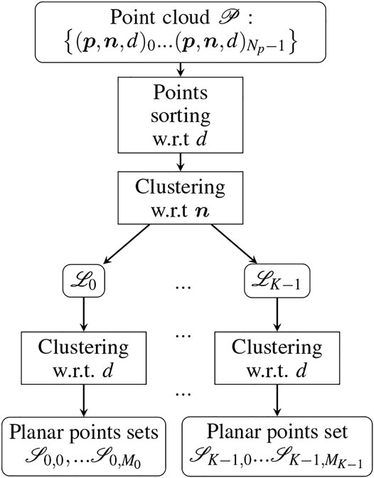
FIGURE 1. Overview of the planar segmentation algorithm. It consists of two clustering phases: the first one is for the normals’ space, and the second one separates parallel planes.

${\mathcal{L}}_k$ stands for the kth set of points P, k ∈ [0, K−1], with similar norm vectors. To finish, ${\mathcal{S}}_{k,m}$ is the notation used for the mth (with m ∈ [0, M_k−1]) set of points in ${\mathcal{L}}_k$ which share the same properties n and d. Notice in ${\mathcal{S}}_{k,m}$, points do not necessary form a connected component but belong to the same planar structure in the real scene. The planar segmentation consists in detecting these sets ${\mathcal{S}}_{k,m}$ (referred to planar structures for sake of simplicity).

The segmentation is performed in two steps. First, the normal vectors are clustered with respect to their orientation using an adaptation of the K-means algorithm Jain (2010) that is described in Section 3.3. For each orientation category, a second clustering (detailed in Section 3.4) is made according to d, in order to separate parallel surfaces, that is planes of similar orientation located at different distances. This is detailed in Section 3.4.

In terms of implementation, two independent threads are used, one for the data pre-processing (storing, normals computation), the other one for the segmentation itself. The first thread computes the normal vectors at each point of the surfaces. Concerning the sorting detailed in Section 3.2, the data are divided into two groups (as shown by Figure 1), depending on whether d is lower or higher than the mean distance $\bar{d}$ computed on the whole point cloud. Here also, this allows to use two threads for the sorting.

3.2 Points Sorting

The input points are sorted using a tree sort algorithm. First, each descriptor P is stored in a binary tree $\mathcal{T}$. The insertion of a descriptor P in a node is made using the distance d as comparison criterion. If d is inferior to the current node d value, then P is inserted into the left child of the node, otherwise, it is inserted into the right one. The list is then sorted by recursively browsing the binary tree $\mathcal{T}$ starting by the left. The mean complexity of this sorting method is O [n log(n)]. The best benefits of the algorithm in terms of performance, are obtained for large amount of data. Consequently, the whole point cloud is sorted first, before creating any cluster, instead of performing one sorting per cluster. In this way, the probability to build an unbalanced tree is minimized, which would lead to a complexity of O(n²) for the spatial sorting. Moreover, the sorting algorithm is easier to parallelize on different threads of equal workload.

3.3 Normals Clustering

The normals clustering is a K-means algorithm Celebi et al. (2013) which is constrained by predefined centroids related to the main planar surfaces that can be found in the building. Assuming the building structure is aligned on a Euclidean grid, the normal vectors of the walls candidates have six possible orientations, one for each axis direction. By starting the capture in front of a wall, the reference frame R₀ is aligned to this Euclidean grid, and the normal vectors for the walls, the ground and the ceiling are along the different axes of R₀.

The original K-means algorithm has been adapted so that it can classify the input normal vectors into at most K classes (K = 6), but can use less classes. Moreover, only points that have a normal vector close to one of the R₀ axes will be considered. It starts by the initialization with the centers $\widehat{{\mathit{o}}_k},k\in [0,K-1]$, corresponding to the six possible orientations aligned with axes u_x, u_y, u_z. These centers are refined to match the actual orientation of the normals when R₀ is not perfectly aligned with the building structure. Let {o_k/k ∈ [0, K−1]} be the final centers (i.e., the mean characteristics of the clusters), and ${\mathcal{L}}_k$ the labeled set where each element of $\mathcal{P}$ is labeled with the corresponding class label k ∈ (0, K−1)⁴.

First of all, each o_k is initialized with the corresponding $\widehat{{\mathit{o}}_k}$, and ${\mathcal{L}}_k$ is initialized with the elements of $\mathcal{P}$ labeled with + ∞. Then, for each iteration of the algorithm, a first loop iterates over each element $(\mathit{p},\mathit{n},d)\in {\mathcal{L}}_k$ and compares them to each center $\widehat{{\mathit{o}}_k}$. If the Euclidean distance Δ_k = δ(n, o_k) is under a threshold ɛ_n, then k is kept as a candidate label. The argmin value k₀ for the candidate labels is kept if it exists. Otherwise, the label is set at + ∞ and the corresponding point data is pruned from the process.

Once each element of ${\mathcal{L}}_k$ has been labeled, each o_k is updated with the mean normal value of the elements of ${\mathcal{L}}_k$ labeled with k. If no element of ${\mathcal{L}}_k$ is labeled with k, then o_k is set to (0, 0, 0).

This process is repeated N times. Similarly, the process could be repeated until convergence. This is a form of constrained E-M approach.

In terms of implementation, since the clustering is made independently on each point, the work can be made by several threads, for instance four threads in this work. We have also used the SIMD4 instructions of the processor to accelerate the execution. Note that Euclidean distance has been preferred to angular distance, because products and sums are faster to compute (and even faster in SIMD) than trigonometric functions.

3.4 Distance Clustering

After normals clustering, a maximum of K clusters ${\mathcal{L}}_k,k\in [0,K-1]$ is formed. For each of these clusters, points have to be separated into parallel planes. Each cluster ${\mathcal{L}}_k$ contains L_k points to be sorted. Let l ∈ [0, L_k−1] be the index of the points inside a cluster ${\mathcal{L}}_k$. In each cluster ${\mathcal{L}}_k$, M_k planar structures have to be determined. Let ${\mathcal{S}}_m$ with m ∈ (0, M_k−1) denote the mth set of points forming a planar structure in ${\mathcal{L}}_k$.

First of all, in each set ${\mathcal{L}}_k$, the L_k points P_l(p_l, n_l, d_l) are sorted by ascending distances d_l. Once sorted, the clustering is straightforward using a DBSCAN method. Subsequent points P_l−1 and P_l are considered as belonging to the same structure ${\mathcal{S}}_m$ when they have close distances, that is when the deviation between their distances |d_l−d_l−1| is less than a threshold ɛ_d. Otherwise, a new plane object is created and initialized with P_l.

3.5 Parameters

Table 1 shows the values of the parameters used to perform the planar segmentation.

TABLE 1

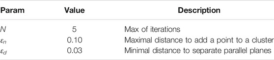
TABLE 1. Parameters for the planar segmentation.

Since the algorithm is fast to converge, a maximum number of iterations N = 5 is enough for the K-means algorithm. The distance ɛ_n has been fixed to 0.10, so normal vectors that are not aligned with the initial frame R₀ are not added to any cluster. The parameter ɛ_d has been set to 0.03. This value is limited by the precision of the depth sensor and the algorithm. Figure 2 shows a few examples of the final segmentation process. The left column shows images from the scene to be reconstructed, while the right column shows the segmentation results, where a different color is given to each plane category.

FIGURE 2

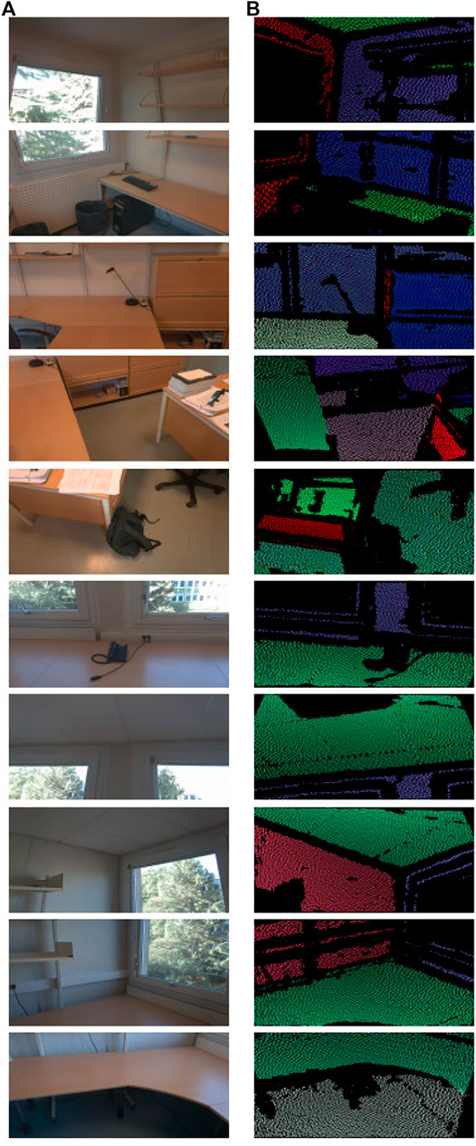
FIGURE 2. Planar segmentation using our method. (A): RGB images of the scene to be segmented. (B): representation of the corresponding 3D points cloud with one color per plane orientation. Only the planes that are aligned with the building structure are detected.

4 From Temporal Matching to the Export of the Model

The current planes are matched with the planes detected in the previous frame. Thus, similar planes are merged and their geometric characteristics are updated, leading progressively to a 3D model of the whole scene. This section first describes the creation and the update of the 3D model, and then explains how the recognition of walls, ground or ceiling is made.

4.1 Planes Matching

All this process is based on the ability to match the currently detected planes (at time t) to the previous ones (at time t−1). Using a motion tracking algorithm, all the 3D coordinates are expressed in a same reference frame R₀.

The method described in Arnaud et al. (2018) is used to match similar planes. For each cluster $\mathcal{S}$ extracted in the previous planar segmentation, the histograms of each parameter, i.e., n_x, n_y, n_z, d, are computed (Figure 3). In theory, all points of $\mathcal{S}$ have the same parameters, while in practice they are distributed following a normal law around the actual parameters. These distributions are used to create a unique identifier ID for each plane, which is used to store the plane in a hash table. Thus the memory is dynamically allocated when new data is available. This identifier ID is built using the four mean values ID = (μ_x, μ_y, μ_z, μ_d) of the distributions of n_x, n_y, n_z, d on the corresponding planar surface. Thus, when a new plane is detected in the current frame, its statistical characteristics are used either to retrieve the previous corresponding plane when it exists with a complexity O(1), or, to create a new plane and the corresponding entry in the hash table.

FIGURE 3

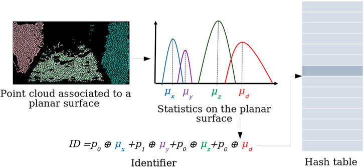
FIGURE 3. Illustration of the hash table. On the left: a point cloud segmented into three planar surfaces. For each planar surface, four histograms are computed. The statistics are used to build an identifier that is used as a key to address the hash table.

4.2 Drifts Correction

The estimation of the global position of the tablet is performed natively using a Visual Inertial Odometry algorithm Li and Mourikis (2012). However, there are still positioning errors that accumulate over time, causing imprecise temporal matching. To correct these possible drifts, an accelerated version of the Iterative Closest Point (ICP) algorithm Besl and McKay (1992) has been implemented.

Let ${\mathcal{P}}_t$ and ${\mathcal{P}}_{t+1}$ be two point clouds captured respectively at times t and t + 1. Each point $P\in \mathcal{P}$ is described by its spatial position p, its color c and its normal vector n. ICP consists in iteratively searching for correspondences between two points clouds and in estimating the affine transform that minimizes a global distance. Our variant of the ICP, described hereafter, accelerates the process by a fast sorting, a pruning of the points that are too far to be considered as homologous, and by exploiting a distance based on location, color and geometry.

4.2.1 Finding Correspondences

For each point in ${\mathcal{P}}_{t+1}$, a match is searched in ${\mathcal{P}}_t$. Considering that ${\mathcal{P}}_{t+1}$ and ${\mathcal{P}}_t$ are nearly aligned, two points $P^{\prime }\in {\mathcal{P}}_{t+1}$ and $P\in {\mathcal{P}}_t$ can be considered for matching if their distance δ(P′, P) is under a threshold ɛ.

Assuming a small movement of the device in the time interval (t, t + 1), the correspondences are searched in a local neighborhood ${\mathcal{W}}_{P,u,v}$ around each point P indexed by (u, v)5.

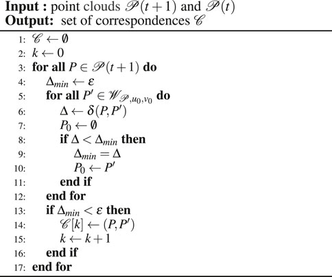
The Algorithm 1 details the procedure for creating a set of correspondences $\mathcal{C}$. Two points P, and P′ are matched if they are similar in terms of location p, color c and normals n, according to the following similarity function δ(P, P′):

$\delta (P,P^{\prime })=\frac{{\omega }_p{\delta }_p(\mathit{p},{\mathit{p}}^{\prime })+{\omega }_c{\delta }_c(\mathit{c},{\mathit{c}}^{\prime })+{\omega }_n{\delta }_n(\mathit{n},{\mathit{n}}^{\prime })}{{\omega }_p+{\omega }_c+{\omega }_n}$

where δ_p, δ_c and δ_n stand for Euclidean distances, computed respectively on spatial location, color and normals. The weights ω_p, ω_c and ω_n are used to give more or less importance to each component.

Algorithm 1 Correspondences searching between two ordered point clouds.

4.2.2 Alignment of the Point Clouds

Then, the two points clouds are aligned geometrically. To this end, the homography transform is estimated. First, the translation T is estimated as the distance between the centroids o′ and o of the spatial positions of ${\mathcal{P}}_t$ and ${\mathcal{P}}_{t+1}$. Then, the rotation R is estimated by computing the mean rotation required to align the normal vectors on their mean normal vector.

4.3 Estimating the Boundaries of Each Plane

Once the point cloud has been separated into different planar structures, each of them can be represented by its area and its boundaries. Among the various possible techniques, two solutions have been considered, as illustrated by Figure 4.

FIGURE 4

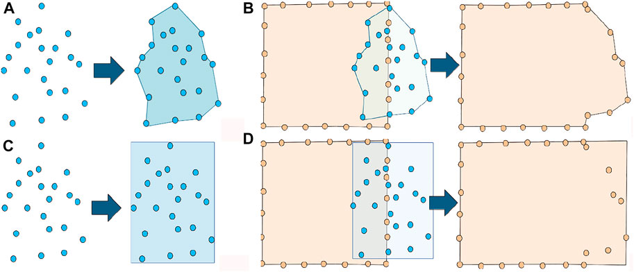
FIGURE 4. Two techniques considered for plan boundaries. The first one consists in computing the full concave hull of each cluster after the segmentation stage (A), and then in repeating this algorithm in order to merge this cluster (detected at time t + 1) with one of the previous clusters (detected at time t) (B). The second technique consists in computing the minimal bounding box of a cluster (C), and to update it after merging with a previous cluster (D).

The first one (Figures 4A,B) consists in computing and updating the full concave hull of a plane using the KNN-based method developed by Moreira and Santos (2007). In the latter, the concave hull is defined as a polygon that best describes the region occupied by a set of points in a plane, i.e., the minimal envelope or the footprint of these points. This technique allows the modeling of walls of non-rectangular shape, but has two disadvantages. First, the concave hull is a growing list of points, and the spatial resolution and growth are limited. In addition, this algorithm is time consuming. The second option, illustrated by Figures 4C,D, consists in using the minimal bounding box of the planes, which is satisfactory when walls are rectangular, as it is the case in our work.

4.4 Walls and Openings Identification

First, the height H of the room is computed. This is made by finding the planes corresponding to the ground and the ceiling, i.e., the planes that are orthogonal to the z axis. The floor and ceiling are respectively the lowest and highest planes. Then, all of the planes that are orthogonal to the ground are considered as potential walls. This is confirmed when its height is at least 80% of H. Examples of walls detection are presented in Figure 5.

FIGURE 5

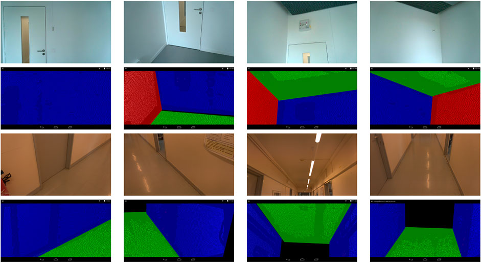
FIGURE 5. Examples of walls identification. The ground and ceiling are displayed in green color, walls are drawn in blue and red.

Once the structural planes identified, the openings (i.e., doors and windows) are detected by assuming that windows are transparent and doors are open. Therefore, the infrared light are not reflected Figure 6A. Thus, the openings appear as void rectangles, i.e., areas for which no input data is available. Each wall is analyzed individually in 2D, and each dimension is sub-sampled as described in Figure 6B. The rectangular shapes are detected using the ratio of the size (number of pixels) of the black area over the size of the minimal bounding box (Figure 6C). A region is considered as an opening when the ratio is close to 1.

FIGURE 6

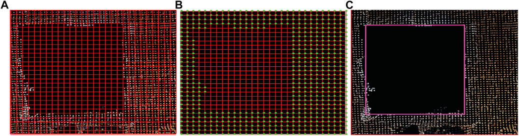
FIGURE 6. Illustration of the openings detection. (A) Infrared light is not reflected by glass. (B) Sub-sampling of the data. (C) Detection of the minimal bounding box.

4.5 Exporting the Model to a CAD Software

After processing, the information needed to create a 3D model are exported in a. xml file. For each wall or opening, the following parameters are saved in this file: an identifier, the coordinates of its four corners and the orientation. The resulting 3D model can be edited in the CAD software, for example to plan renovation and decorating works (Figure 7). In the application Plan 3D Energy that we developed (Figure 8) with the society RPE, it is possible to specify the characteristics of the building and the materials for each wall and each opening. These estimations, together with the data that our algorithm can provide, it is possible to estimate the energy losses of the room6, and consequently its energetic performances. It represents a useful tool to sensitize users to make energetic responsible choices regarding their interior renovation works. To evaluate the quality of the energetic estimation when using the proposed system, five scans of a room have been performed, and the energy losses are compared to the estimations made with the real dimensions (310kWhm⁻²year⁻¹, letter E). Using our 3D models, the estimated energetic performances are 306kWhm⁻²year⁻¹ in average, and systematically lead to the same letter E.⁵

FIGURE 7

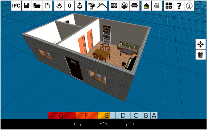
FIGURE 7. Example of applications: decorating, evaluating energetic performances.

FIGURE 8

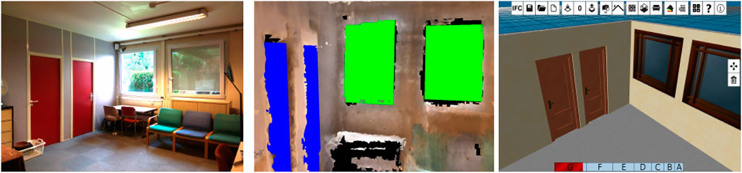
FIGURE 8. A 3D model viewed in the software Plan 3D Energy.

5 Evaluations

This section presents the evaluations of the planar segmentation algorithm used as a basis for wall detection.

5.1 Material

Developments were made on a Google Tango Yellowstone tablet, equipped with a Nvidia Tegra K1 processor and 4 GB RAM, and running on Android 4.4. It embeds a depth sensor and a motion tracking algorithm based on Virtual Inertial Odometry Li and Mourikis (2012).

5.2 Evaluation of the Precision and Reliability

Both the reliability and the precision of the planes detection are evaluated. For this purpose, the device is first put in front of an empty wall at a fixed distance x. Then, another planar surface is put between the device and the wall, at a fixed distance D from the wall. Figure 9 illustrates the setup. For each configuration, the procedure is tested on 100 successive point clouds. Two measures are used: the number n of times the algorithm detects exactly two planes; if so, the distance d between the two detected surfaces. The results are presented in Table 2.

FIGURE 9

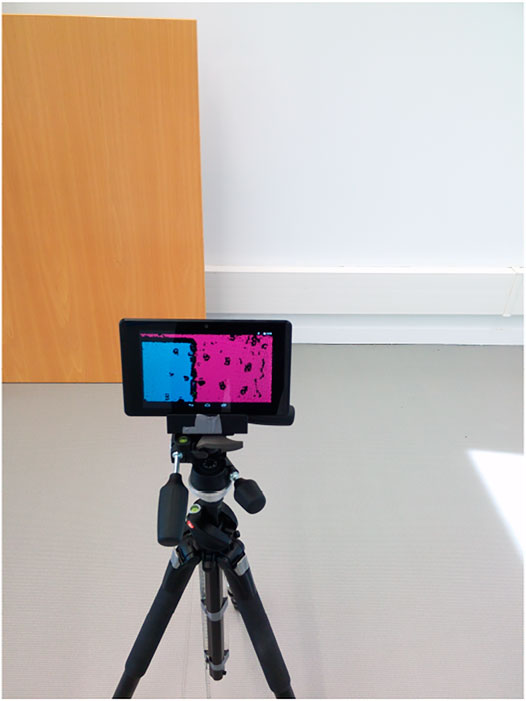
FIGURE 9. Setup used for evaluation precision.

TABLE 2

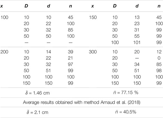
TABLE 2. Results of the evaluation of the segmentation algorithm for 100 measures. x represents the distance between the tablet and the furthest plane, D the real distance between the two planes and d the measured one. All these distances are expressed in centimeters. n represents the number of valid measured frames for each condition.

The mean error $\bar{\delta }$ for the estimation of D is 1.46 cm, and the mean percentage of frames where exactly two planes are detected $\bar{n}$ is 77.15%. In comparison, in Arnaud et al. (2018), the error was approximately 2.1 cm, and two planes were correctly detected in 40.5% of the cases. More detailed results are given in Figure 10.

FIGURE 10

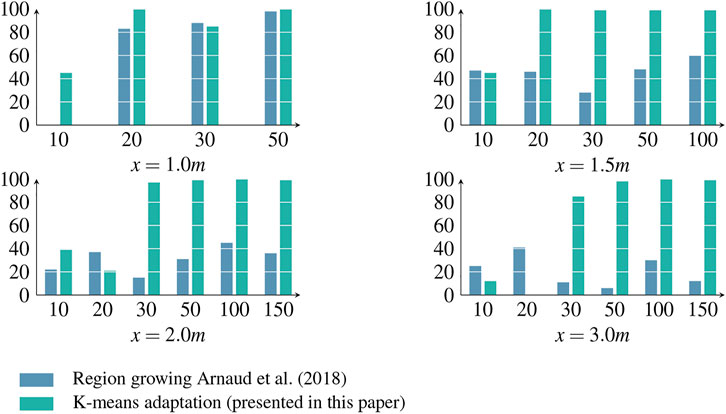
FIGURE 10. Comparison of the percentage of frames where two planes were detected n (ordinate axis) for both planar segmentations algorithms depending on the inter-planes distance D (abcissa) for each different configuration of x.

Thus, it can be seen that the clustering method provides a better precision in most cases, and is able to distinguish parallel walls with a high reliability if their inter-plane distance is up to 10 cm. For each algorithm, some errors occur for low inter-planes distances D. This is due to the norms estimation, which is not accurate enough on the edges of the depth map. Most failures occur when two planes are close from each other. In terms of execution time, the clustering approach is 5–10 times faster than the growing regions strategy.

5.3 Evaluation of the 3D Model

Once the scan is made, we have a 3D model representing a set of walls and their geometric dimensions. Then the estimated dimensions can be compared with the real ones, measured by using a laser meter.

The three rooms used for evaluation are shown in Figure 11.

FIGURE 11

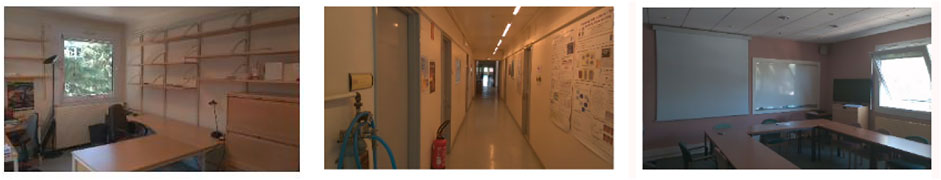
FIGURE 11. Images of the rooms used for evaluation.

First, the rooms are scanned, the walls are identified, as explained in Section 4.4, and their dimensions are estimated. The experience is repeated 10 times for each room. The Table 3 synthesizes the results using the precision and execution times for three methods. The first one is the accelerated implementation of CHISEL algorithm Klingensmith et al. (2015), with the use of RANSAC for planar detection Arnaud et al. (2016). This version does not run in real-time and the execution time varies from 200 to 500 ms. Concerning the algorithm detailed in Arnaud et al. (2018), which estimates the 3D mesh of the room before achieving the bottom-up segmentation, it just reaches real-time execution. The mean error is approximately 5% of the real dimensions, with a maximum error of 25%. The maximum error is obtained for the meeting room, where the ceiling lights distort the measurements of the depth sensor. The proposed approach reduces the errors, as also shown in Table 2 and it is faster. Note also that the furniture in the scenes (the clutter) do not harm the detection of the walls because each wall is partly visible. Of course, errors could occur in the following situations: when a wall is totally occluded from the floor to the ceiling by a piece of furniture, when the room is not square or rectangular.

TABLE 3

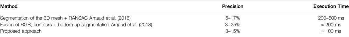
TABLE 3. Synthetic comparison of three different methods. The precision is given as a percentage w.r.t the real dimensions.

5.4 Evaluation of the Usability

Some experiments have been conducted to evaluate the usability of the system. First, we compare the time needed for manually measuring the dimensions of a room using a laser meter, with the time needed to scan and generate the model with the proposed system. Ten people of different ages, genders and professions participated to the experiment. 419 (±73) seconds were needed to scan the room with the laser meter, whereas it took 247 (±44) seconds to get the 3D model when using the proposed system. Let us underline that the 419 s do not include the modeling stage, i.e., entering the dimensions manually in a CAD software. Figure 12 shows an example of sketch made by one the user after measuring the room. We applied the SUS questionnaire Brooke (1996) to evaluate the usability of the system. Users answer 10 questions formulated in such a way that they are generic and apply to any type of service or system. A score close to 100 indicates excellent satisfaction.

FIGURE 12

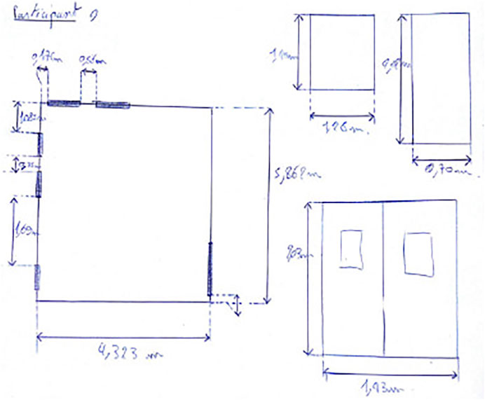
FIGURE 12. Example of sketch drawn by an user during the usability experiment.

Using a SUS questionnaire Brooke (1996), a mean usability score of 75 was obtained which correspond to a good satisfaction, which shows that the application can be easily understood by inexperienced users. Among the 10 participants, two users found that the use of the tablet did not bring any advantage compared to a manual measure. The usability score was higher than 75 for seven participants, with a maximum score of 93 for three persons.

6 Conclusion and Future Works

This paper has described an application that runs on a tablet equipped with a depth sensor that generates and updates a 3D model of an indoor environment. The 3D model is built in real-time and uses exclusively the computing capabilities of the tablet. This has been made possible by making assumptions (the building structure is aligned on an Euclidean grid), by using adapted data structures (hash tables and binary trees), by combining a fast planar segmentation using hierarchical clustering, by achieving code acceleration (SIMD) and multi-threading.

Our evaluations show that the planar segmentation algorithm is able to distinguish parallel planes if they are separated by more than 10 cm, with a very high accuracy, and that the planes placement accuracy is less than 2 cm. Compared to previous work, the precision and speed have been significantly improved. This accuracy can be further improved by using a more accurate depth sensor. Some user experiments have also shown that it takes approximately twice less time to scan a room compared to the measurement using a laser meter. A usability score of 75 was obtained. In addition, the 3D model can be edited in a CAD software, for example to estimate the energetic performances, to plan renovation and decorating works.

One of the perspectives of this work is the improvement of the proposed application, while maintaining the real-time performance, which is key for a good user experience. Concerning the 3D planar segmentation, it would be interesting to extend the work to more complex rooms where walls are not perpendicular, or when some of the walls are totally made of glass. Regarding the analysis of the walls, the key elements of the rooms, such as openings, could be made by using a semantic segmentation Zhang et al. (2013) or by recent deep learning techniques. To finish, the parameters of the algorithms have been selected manually. Even if they are satisfactory for all the scenes we studied, a calibration is a component that could be useful in other contexts (in order to update the parameters automatically).

In a more technical concern, the proposed application has been developed on Android for the Tango Platform, which has a depth sensor and a visual odometry system. This is unfortunately not the case for all devices, but more and more Android models are proposed at an affordable price Taneja, 2020). When not available on the device, a visual odometry algorithm can be installed Li and Mourikis (2012). More generally, the future application could be available in different versions, depending on the targeted device and its components. This requires consequent engineering work, which is out of the scope of this work.

Data Availability Statement

The original contributions presented in the study are included in the article/Supplementary Material, further inquiries can be directed to the corresponding author.

Author Contributions

AA: writing, coding, experiments MG: writing, supervision MA: writing, supervision.

Funding

This work was funded by Rénovation Plaisir Energie (RPE).

Conflict of Interest

The authors declare that the research was conducted in the absence of any commercial or financial relationships that could be construed as a potential conflict of interest.

Publisher’s Note

All claims expressed in this article are solely those of the authors and do not necessarily represent those of their affiliated organizations, or those of the publisher, the editors and the reviewers. Any product that may be evaluated in this article, or claim that may be made by its manufacturer, is not guaranteed or endorsed by the publisher.

Footnotes

¹BIM stands for: Building Information Model.

²CAD for Computer Aided Design.

³https://developers.google.com/ar/.

⁴SIMD for Single Instruction Multiple Data

⁵Note that two coordinates are enough since the points lie on the same planar surface.

⁶The energy losses of one surface is the surface multiplied by its heat transfer coefficient defined by the 3CL10 norm according to the main building features: year of construction, type of insulation, materials of the building.

References

Adan, A., and Huber, D. (2011). “3d Reconstruction of interior wall Surfaces under Occlusion and Clutter,” in 2011 International Conference on 3D Imaging, Modeling, Processing, Visualization and Transmission (IEEE) (IEEE), 275–281. doi:10.1109/3dimpvt.2011.42

CrossRef Full Text | Google Scholar

Arnaud, A., Christophe, J., Gouiffès, M., and Ammi, M. (2016). 3D Reconstruction of Indoor Building Environments with New Generation of Tablets. In VRST ’16 Proceedings of the 22nd ACM Conference on Virtual Reality Software and Technology. 187–190.

CrossRef Full Text | Google Scholar

Arnaud, A., Gouiffès, M., and Ammi, M. (2018). On the Fly Plane Detection and Time Consistency for Indoor Building wall Recognition Using a Tablet Equipped with a Depth Sensor. IEEE Access 6, 17643–17652. doi:10.1109/access.2018.2817838

CrossRef Full Text | Google Scholar

Barbu, A., and Song-Chun Zhu, S.-C. (2005). Generalizing Swendsen-Wang to Sampling Arbitrary Posterior Probabilities. IEEE Trans. Pattern Anal. Machine Intell. 27, 1239–1253. doi:10.1109/tpami.2005.161

PubMed Abstract | CrossRef Full Text | Google Scholar

Besl, P. J., and McKay, N. D. (1992). A Method for Registration of 3-D Shapes. IEEE Trans. Pattern Anal. Mach. Intell. 14, 239–256. doi:10.1109/34.121791

CrossRef Full Text | Google Scholar

Borrmann, D., Elseberg, J., Lingemann, K., and Nüchter, A. (2011). The 3D Hough Transform for Plane Detection in point Clouds: A Review and a New Accumulator Design. 3D Res. 2, 1–13. doi:10.1007/3dres.02(2011)3

CrossRef Full Text | Google Scholar

Brooke, J. (1996). SUS-A Quick and Dirty Usability Scale. Usability Eval. industry 189, 4–7.

Google Scholar

Celebi, M. E., Kingravi, H. A., and Vela, P. A. (2013). A Comparative Study of Efficient Initialization Methods for the K-Means Clustering Algorithm. Expert Syst. Appl. 40, 200–210. doi:10.1016/j.eswa.2012.07.021

CrossRef Full Text | Google Scholar

Coughlan, J. M., and Yuille, A. L. (1999). “Manhattan World: Compass Direction from a Single Image by Bayesian Inference,” in Computer Vision, 1999. The Proceedings of the Seventh IEEE International Conference on (IEEE) (IEEE), 941–947.Vol. 2

CrossRef Full Text | Google Scholar

Deng, Z., Todorovic, S., and Jan Latecki, L. (2017). Unsupervised Object Region Proposals for RGB-D Indoor Scenes. Computer Vis. Image Understanding 154, 127–136. doi:10.1016/j.cviu.2016.07.005

CrossRef Full Text | Google Scholar

Erdogan, C., Paluri, M., and Dellaert, F. (2012). “Planar Segmentation of RGB-D Images Using Fast Linear Fitting and Markov Chain Monte Carlo,” in Computer and Robot Vision (CRV), 2012 Ninth Conference on (IEEE) (IEEE), 32–39. doi:10.1109/crv.2012.12

CrossRef Full Text | Google Scholar

Ester, M., Kriegel, H.-P., Sander, J., and Xu, X. (1996). A Density-Based Algorithm for Discovering Clusters in Large Spatial Databases with Noise. in. Proceedings of the Second International Conference on Knowledge Discovery and Data Mining (KDD96) 96, 226–231.

Google Scholar

Fulkerson, B., Vedaldi, A., and Soatto, S. (2009). “Class Segmentation and Object Localization with Superpixel Neighborhoods,” in Computer Vision, 2009 IEEE 12th International Conference on (IEEE) (IEEE), 670–677. doi:10.1109/iccv.2009.5459175

CrossRef Full Text | Google Scholar

Grilli, E., Menna, F., and Remondino, F. (2017). A Review of point Clouds Segmentation and Classification Algorithms. Int. Arch. Photogramm. Remote Sens. Spat. Inf. Sci. XLII-2/W3, 339–344. doi:10.5194/isprs-archives-xlii-2-w3-339-2017

CrossRef Full Text | Google Scholar

Gupta, S., Arbelaez, P., and Malik, J. (2013). “Perceptual Organization and Recognition of Indoor Scenes from RGB-D Images,” in Proceedings of the IEEE Conference on Computer Vision and Pattern Recognition, 564–571.

CrossRef Full Text | Google Scholar

Henry, P., Krainin, M., Herbst, E., Ren, X., and Fox, D. (2012). RGB-D Mapping: Using Kinect-Style Depth Cameras for Dense 3D Modeling of Indoor Environments. Int. J. Robotics Res. 31, 647–663. doi:10.1177/0278364911434148

CrossRef Full Text | Google Scholar

Holz, D., Holzer, S., Rusu, R. B., and Behnke, S. (2011). Robot Soccer World Cup. Springer, Berlin, Heidelberg, 306–317.Real-time Plane Segmentation Using RGB-D Cameras

Google Scholar

Jain, A. K. (2010). Data Clustering: 50 Years beyond K-Means. Pattern recognition Lett. 31, 651–666. doi:10.1016/j.patrec.2009.09.011

CrossRef Full Text | Google Scholar

Jung, J., Hong, S., Jeong, S., Kim, S., Cho, H., Hong, S., et al. (2014). Productive Modeling for Development of As-Built BIM of Existing Indoor Structures. Automation in Construction 42, 68–77. doi:10.1016/j.autcon.2014.02.021

CrossRef Full Text | Google Scholar

Jung, Y., and Joo, M. (2011). Building Information Modelling (BIM) Framework for Practical Implementation. Automation in construction 20, 126–133. doi:10.1016/j.autcon.2010.09.010

CrossRef Full Text | Google Scholar

Kang, Z., Yang, J., Yang, Z., and Cheng, S. (2020). A Review of Techniques for 3D Reconstruction of Indoor Environments. ISPRS Int. J. Geo-inf, 9. doi:10.3390/ijgi9050330

CrossRef Full Text | Google Scholar

Klingensmith, M., Dryanovski, I., Srinivasa, S., and Xiao, J. (2015). Chisel: Real Time Large Scale 3d Reconstruction Onboard a mobile Device Using Spatially Hashed Signed Distance fields. Robotics: Sci. Syst. XI. doi:10.15607/RSS.2015.XI.040

CrossRef Full Text | Google Scholar

Lai, K., Bo, L., and Fox, D. (2014). “Unsupervised Feature Learning for 3D Scene Labeling,” in Robotics and Automation (ICRA), 2014 IEEE International Conference on (IEEE) (IEEE), 3050–3057. doi:10.1109/icra.2014.6907298

CrossRef Full Text | Google Scholar

Lee, D. C., Hebert, M., and Kanade, T. (2009). “Geometric Reasoning for Single Image Structure Recovery,” in Computer Vision and Pattern Recognition, 2009. CVPR 2009. IEEE Conference on (IEEE) (IEEE), 2136–2143. doi:10.1109/cvpr.2009.5206872

CrossRef Full Text | Google Scholar

Li, M., and Mourikis, A. I. (2012). “Improving the Accuracy of EKF-Based Visual-Inertial Odometry,” in IEEE Int. Conf. on Robotics and Automation (ICRA) (IEEE (IEEE), 828–835. doi:10.1109/icra.2012.6225229

CrossRef Full Text | Google Scholar

Liang, Y., He, F., and Zeng, X. (2020). 3d Mesh Simplification with Feature Preservation Based on Whale Optimization Algorithm and Differential Evolution. Ica 27, 417–435. doi:10.3233/ica-200641

CrossRef Full Text | Google Scholar

Macher, H., Landes, T., and Grussenmeyer, P. (2015). Point Clouds Segmentation as Base for As-Built BIM Creation. ISPRS Ann. Photogramm. Remote Sens. Spat. Inf. Sci. II-5/W3, 191–197. doi:10.5194/isprsannals-ii-5-w3-191-2015

CrossRef Full Text | Google Scholar

Moreira, A., and Santos, M. Y. (2007). Concave hull: A K-Nearest Neighbours Approach for the Computation of the Region Occupied by a Set of Points

Google Scholar

Nguyen, A., and Le, B. (2013). 3D point Cloud Segmentation: A Survey. RAM, 225–230. doi:10.1109/RAM.2013.6758588

CrossRef Full Text | Google Scholar

Ochmann, S., Vock, R., Wessel, R., and Klein, R. (2016). Automatic Reconstruction of Parametric Building Models from Indoor point Clouds. Comput. Graphics 54, 94–103. doi:10.1016/j.cag.2015.07.008

CrossRef Full Text | Google Scholar

Papon, J., Abramov, A., Schoeler, M., and Worgotter, F. (2013). “Voxel Cloud Connectivity Segmentation-Supervoxels for point Clouds,” in Proceedings of the IEEE Conference on Computer Vision and Pattern Recognition (IEEE), 2027–2034.

CrossRef Full Text | Google Scholar

Ren, X., Bo, L., and Fox, D. (2012). “Rgb-(d) Scene Labeling: Features and Algorithms,” in Computer Vision and Pattern Recognition (CVPR), 2012 IEEE Conference on (IEEE) (IEEE), 2759–2766. doi:10.1109/cvpr.2012.6247999

CrossRef Full Text | Google Scholar

Schnabel, R., Wahl, R., and Klein, R. (2007). Efficient RANSAC for Point-Cloud Shape Detection. Comp. Graphics Forum 26, 214–226. doi:10.1111/j.1467-8659.2007.01016.x

CrossRef Full Text | Google Scholar

Silberman, N., Hoiem, D., Kohli, P., and Fergus, R. (2012). European Conference on Computer Vision. Springer, 746–760. doi:10.1007/978-3-642-33715-4_54Indoor Segmentation and Support Inference from RGBD Images

CrossRef Full Text | Google Scholar

Swendsen, R. H., and Wang, J.-S. (1987). Nonuniversal Critical Dynamics in Monte Carlo Simulations. Phys. Rev. Lett. 58, 86–88. doi:10.1103/physrevlett.58.86

PubMed Abstract | CrossRef Full Text | Google Scholar

Taneja (2020). A. Top 10 Smartphones with A Dedicated Depth Sensor Camera to Capture Perfect Bokeh Shots. Available at: https://www.cashify.in/top-10-smartphones-with-a-dedicated-depth-sensor-camera-to-capture-perfect-bokeh-shots (Accessed 10 01, 2020).

Google Scholar

Tarsha-Kurdi, F., Landes, T., and Grussenmeyer, P. (2007). Hough-transform and Extended RANSAC Algorithms for Automatic Detection of 3D Building Roof Planes from LIDAR Data. Proc. ISPRS Workshop Laser Scanning 36, 407–412.

Google Scholar

Tatavarti, A., Papadakis, J., and Willis, A. R. (2017). Towards Real-Time Segmentation of 3D point Cloud Data into Local Planar Regions. SoutheastCon 2017 (IEEE), 1–6. doi:10.1109/secon.2017.7925321

CrossRef Full Text | Google Scholar

Verma, V., Kumar, R., and Hsu, S. (2006). “3D Building Detection and Modeling from Aerial LIDAR Data,” in Computer Vision and Pattern Recognition, 2006 IEEE Computer Society Conference on (IEEE) (IEEE), 2213–2220.Vol. 2

Google Scholar

Zhang, D., He, F., Tu, Z., Zou, L., and Chen, Y. (2020). Pointwise Geometric and Semantic Learning Network on 3D point Clouds. Integrated Computer-Aided Eng. 27, 57–75. doi:10.3233/ICA-190608

CrossRef Full Text | Google Scholar

Zhang, J., Kan, C., Schwing, A. G., and Urtasun, R. (2013). Estimating the 3D Layout of Indoor Scenes and its Clutter from Depth Sensors. IEEE Int. Conf. Comp. Vis. (Iccv), 1273–1280. doi:10.1109/iccv.2013.161

CrossRef Full Text | Google Scholar