Price Variance in Hybrid-LCA Leads to Significant Uncertainty in Carbon Footprints

Hybrid Life Cycle Assessment (HLCA) methods attempt to address the limitations regarding process coverage and resolution of the more traditional Process- and Input-Output Life Cycle Assessments (PLCA, IOLCA). Due to the use of different units, HLCA methods rely on commodity price information to convert the physical units used in process inventories to the monetary units commonly used in Input-Output models. However, prices for the same commodity can vary significantly between different supply chains, or even between various levels in the same supply chain. The resulting commodity price variance in turn leads to added uncertainty in the hybrid environmental footprint. In this paper we take international trading statistics from BACI/UN-COMTRADE to estimate the variance of commodity prices, and use these in an integrated HLCA model of the process database ecoinvent with the EE-MRIO database EXIOBASE. We show that geographical aggregation of PLCA processes is a significant driver in the price variance of their reference products. We analyse the effect of price variance on process carbon footprint intensities (CFIs) and find that the CFIs of hybridised processes show a median increase of 6–17% due to hybridisation, for two different double counting scenarios, and a median uncertainty of −2 to +4% due to price variance. Furthermore, we illustrate the effect of price variance on the carbon footprint uncertainty in a HLCA study of Swiss household consumption. Although the relative footprint increase due to hybridisation is small to moderate with 8–14% for two different double counting correction strategies, the uncertainty due to price variability of this contribution to the footprint is very high, with 95% confidence intervals of (−28, +90%) and (−23, +68%) relative to the median. The magnitude and high positive skewness of the uncertainty highlights the importance of taking price variance into account when performing hybrid LCA.

1. Introduction

Both Process- and Input-Output Life Cycle Assessment (PLCA, IOLCA) are common tools to assess the environmental burdens of the local, regional, or global economy (Crawford et al., 2018, and references therein). While PLCA holds the promise of highly detailed assessments, the limited data availability at this level of detail inevitably leads to gaps in the supply chains, and consequently to an underestimation of upstream impacts, also called the truncation error (Suh et al., 2004; Crawford et al., 2018; Ward et al., 2018). IOLCA on the other hand offers a complete supply chain model, however, it lacks the level of detail of PLCA studies.

Hybrid Life Cycle Assessment (HLCA) is considered as a way to mitigate the truncation errors in traditional PLCA, either by completing the system boundary through the use of IO data (Treloar et al., 2000; Lenzen, 2001; Suh, 2004; Suh et al., 2004; Suh and Huppes, 2005), or to improve the precision of IOLCA studies (Treloar, 1997; Lenzen and Crawford, 2009; Crawford et al., 2017). Yet in spite of the potential improvements it has to offer over PLCA and IOLCA, HLCA has yet to see a major uptake in mainstream LCA practice. This is often attributed to the highly manual and time consuming process of linking process- and input-output data. In scientific literature, however, HLCA is becoming more commonly a tool to assess environmental footprints of consumption and services (Larsen and Hertwich, 2009; Lin et al., 2013), as for example the effort to promote local sustainability. That is, sustainability on a city or regional level, requires higher detail than the average national input-output tables can provide (Larsen and Hertwich, 2009). On the other hand, the requirement of higher detail assessments also leads to the uptake of PLCA for consumption-based accounting (Kalbar et al., 2016; Froemelt et al., 2018; Sala and Castellani, 2019). This underlines the need for streamlined and automated hybridisation methods and tools. As such, multiple projects have been working on automating the compilation of hybrid databases (Crawford et al., 2017; Yu and Wiedmann, 2018; Agez et al., 2019; Stephan et al., 2019) in order to enhance the uptake of hybrid LCA.

Although consensus seems to exist in literature on the shortcomings of both PLCA and IOLCA as tools to assess the environmental impacts of product systems, the use of IO data to expand the system boundary of PLCA and fill in the data gaps of a typical Process Life Cycle Inventory is not completely undisputed. Some authors argue that the inclusion of aggregated IO data can lead to less accurate results due to the introduction of aggregation errors with the IO data (Yang et al., 2017). Others argue that the aggregation error introduced with the inclusion of IO data is smaller than the truncation error of PLCA alone (Pomponi and Lenzen, 2018). Estimating the magnitude of truncation error in PLCA studies remains a topic of active research (Junnila, 2006; Majeau-Bettez et al., 2011; Ward et al., 2018; Perkins and Suh, 2019), which is a natural consequence of the lack of an accurate and complete system description or “true” environmental footprints. Hence, in practice, hybrid LCA or IOLCA are being used as complete system descriptions to estimate the magnitude of the truncation error of PLCA systems (Ward et al., 2018, and references therein).

More recently Perkins and Suh (2019) framed the discussion on the “correctness” of HLCA vs. PLCA as an accuracy vs. precision debate: PLCA providing high levels of “precision” with the high detail LCI data, but lacking “accuracy” due to truncation errors. They argue that while HLCA can improve the accuracy through the inclusion of IO data, this leads to a lower, albeit reasonable, level of precision due to the higher uncertainty within the IO data sets (Majeau-Bettez et al., 2011). Using a case study of a jacket, based on a study published by the Mistra Future Fashion Consortium (Roos and Zamani, 2015), they show that the inclusion of IO data increases the mean life cycle greenhouse gas (GHG) emissions by 38%, while the relative standard deviation of the results only increases by 3–4%.

Various methods exist for the hybridisation of process- and input-output data which each have their pros and cons (Islam et al., 2016; Crawford et al., 2018). However, one aspect which current implementations all have in common, is their reliance on product- (or service-) price information to deal with unit conversion between the physical units of PLCA databases and the monetary units in IO tables. We note that although physical input-output models are being advocated and developed (Merciai and Schmidt, 2018; Bruckner et al., 2019; Towa et al., 2020), current physical models either do not offer a complete sectoral coverage (Bruckner et al., 2019) or rely on PLCA data to determine sectoral input structures (Merciai and Schmidt, 2018), making them unsuitable for a complete hybrid database covering global supply chains.

In their implementation of an automated system-wide hybridisation, Yu and Wiedmann (2018) investigate the impact of the uncertainty of commodity prices. Assuming, for each process, a normal distribution with a coefficient of variation (CoV) of 30%, they find that the per process carbon footprint intensity (CFI) varies between −31 and +33%, with an average relative uncertainty range of −4.7–+5.1%, and a small variation between the stricter and the less strict double counting correction strategies they applied. These price variance induced uncertainties are, however, significantly smaller than the estimated truncation error corrections themselves, with the hybrid CFI's being 21–32% higher than their corresponding PLCA counterparts.

In practice, commodity prices are subject to a wide range of factors and depend strongly on the buyer-seller relationship. Market dynamics may also lead to price variation throughout a given calendar year, which is the temporal resolution of input-output data. In specific case studies such as the one from Perkins and Suh (2019), one might assume that the practitioner may find reasonable price range estimates for the most important products from processes that are complemented with input-output data. Although the contribution of processes to the overall footprint will likely decrease with each layer of the supply chain, the number of processes that are hybridised in each consecutive layer will likely increase. This means that reliable price ranges are required for all processes in the PLCA database that will take inputs from the input-output table.

Yu and Wiedmann (2018) point out that reliable price information is crucial in hybrid LCA, but that obtaining prices for all reference products in an entire LCA database is an enormously time consuming task. And while they have shown that a theoretical price variance has indeed a significant impact on the footprints of individual processes, the question of how large this uncertainty is in reality remains unresolved. Therefore, this paper takes a statistical approach to investigate the magnitude of this problem, using data on trade flows from the BACI trade database (Gaulier and Zignago, 2010) to model price distributions for the reference products of LCA processes. We first analyse the statistical uncertainty on the process level, before using a consumption basket to show the effect of price uncertainty on a consumption footprint. For this we use the PLCA part of the model of Swiss household consumption of Froemelt et al. (2018). This model is based on the Swiss household consumption survey (HBS 2012–2014; Bundesamt für Statistik, 2013) and the process life cycle inventory ecoinvent (Steubing et al., 2016; Wernet et al., 2016). For the hybrid model we use the open source hybridisation package pyLCAIO (Agez et al., 2020) to create a complete hybrid model of ecoinvent 3.5 and the input output database EXIOBASE v3.6 year 2012 in a product-by-product industry-technology construct (Stadler et al., 2018).

This paper is structured as follows: In section 2, we first discuss the hybrid LCA model (section 2.1) and the influence of prices on the hybrid model (section 2.2). We then introduce the BACI trade data (section 2.3), and the mapping of ecoinvent process reference products to trade flows (section 2.3.1). While not all relevant ecoinvent reference products/services are captured in the BACI trade data, we use proxy data to estimate the price uncertainty which is described in section 2.4. The Swiss household consumption data is introduced in section 2.5 and the Monte Carlo simulation process in section 2.6. In section 3, the results of the Monte Carlo simulations are presented before discussing them in section 4.

2. Materials and Methods

2.1. Hybrid Model

Various hybridisation methods have been proposed and applied in literature, and can be categorised into four different types: Tiered-, Path Exchange-, Matrix Augmentation-, and Integrated hybrid (Crawford et al., 2018, and references therein). Crawford et al. (2018) conclude that only the Path Exchange and Integrated hybrid have a rigorous mathematical framework in place, and therefore provide the most comprehensive approach for the hybridisation of process- and input-output data. Both of these methods have seen efforts to streamline and automate the hybridisation of process- and input-output data in recent years (Bontinck et al., 2017; Crawford et al., 2017; Yu and Wiedmann, 2018; Stephan et al., 2019; Agez et al., 2020). So far the authors are aware of only two studies that hybridised a complete process database with a complete input-output database: the hybridisation of the Australian Life Cycle Database¹ with data from the Australian Industrial Ecology Virtual Laboratory² (Yu and Wiedmann, 2018), and the hybridisation of the ecoinvent life cycle inventory database v3.5 (Steubing et al., 2016; Wernet et al., 2016) with the multi-regional input-output dataset EXIOBASE 3 (Stadler et al., 2018; Agez et al., 2020). The mathematical framework used by both of these efforts is given by Equation (1):

$\begin{array}{ll}{q}_h=\left(\begin{array}{cc}{B}^{\text{lca}}& B^{\text{io}}\end{array}\right){\left[I-\left(\begin{array}{cc}{A}^{\text{lca}}& C^{\text{d }}\\ C^{\text{u}}& A^{\text{io}}\end{array}\right)\right]}^{-1}\left(\begin{array}{c}{y}^{\text{lca}}\\ y^{\text{io}}\end{array}\right),& \left(1\right)\end{array}$

where:

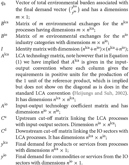
It is often argued that the effect of C^d on the result of the hybrid analysis is minimal while requiring a significant effort to determine and therefore excluded by many authors using the integrated hybrid method (Crawford et al., 2018). However, Suh (2006) argues in a reply to Peters and Hertwich (2006) that even though the effect of C^d on the final footprints will be very small, there are cases where the effect would be significant and C^d should not be disregarded a priori. We note that both Yu and Wiedmann (2018), Agez et al. (2020) do not include C^d and for this reason refer to their method as a tiered hybrid as opposed to the interconnected and balanced system proposed by Suh (2004). Following the classification of Crawford et al. (2018), we use the term “integrated hybrid” as a description of the mathematical framework in this work.

One of the main challenges in the hybridisation of PLCA and IO data is the issue of double counting inputs in the supply chain (Lenzen, 2009; Crawford et al., 2018; Agez et al., 2019). That is, if inputs into a process' supply chain are already accounted for in the process description, these should not be included “again” from the IO data. The Path Exchange method forgoes this problem by “disaggregating” the IO matrix into a series of mutually exclusive nodes by means of a structural path analysis and then replacing individual nodes of these supply chains with product specific process data (Treloar, 1997; Lenzen and Crawford, 2009; Crawford et al., 2017). Agez et al. (2019) discuss the issue of double counting in the integrated hybrid framework and the different existing strategies to deal with them. Moreover, they propose a method to correct for double counting that relies only on the practitioner's general knowledge of the process database. They dub this the “similar technological attributes method” (STAM).

In this work we build upon the open source hybridisation package pyLCAIO³ published by Agez et al. (2020), which is an implementation of the integrated hybrid for the ecoinvent and EXIOBASE databases, applying either the STAM or the “binary” double counting correction strategy. The upstream cut-off matrix is calculated according to:

$\begin{array}{ll}{C}^u=\text{Corr}◦\left[A^{\text{io}}(H◦\text{Geo})\widehat{\Pi }\right].& (2)\end{array}$

Here, Corr stands for the double counting correction strategy being applied (either STAM or binary), A^io is the commodity-commodity multi-regional technology coefficient matrix, H is the concordance matrix matching the processes to the commodity groups in the MRIO database, Geo is a region concordance matrix handling the disparity in geographical resolution between the two databases, $\widehat{\Pi }$ is the “diagonalised” vector of prices for reference products in the process database, and ◦ is the Hadamard or “element-wise” product. For further details regarding the construction of H, Geo, or the STAM or binary double counting correction method, we refer the reader to Agez et al. (2020).

2.2. Product Price Variability

Due to the use of different units in process life cycle inventories (physical units) and input-output tables or their underlying supply and use tables (monetary units), linking process data to IO tables relies on a unit conversion that represents the average price of the commodities in a given region. As we can see in Equation (2), the elements of the cut-off matrix in the column of a given process, and with that its direct requirements from the IO sectors, are directly proportional to the price of the process' reference product. However, these prices will vary depending on the specific buyer-seller relations, such as that a customer placing a large order is likely to pay less per unit or per volume than one placing a smaller order.

Reference product prices in ecoinvent activities should be regarded as an estimate for the basic price of the commodity, that is the actual cost of the production including labour and profit, or put differently, the purchaser price minus trade margins, transport costs, taxes, and or subsidies. These prices are collected and/or estimated from various sources and consecutively “balanced” in an iterative process such that the sum of an activity's inputs never exceeds the value of the activity's output, resulting in a “minimum price” estimate (Moreno Ruiz et al., 2016). We note that while this last step ensures a minimal basic consistency, value added and expenses for waste treatment are not included in this calculation which will likely lead to an underestimation of these prices.

The main purpose of price information in ecoinvent is that of economic allocation, meaning that commodity prices have direct influence on the allocation results and, consequently, the impact results. Although not all co-production processes use economic allocation, the high level interconnectivity means that a change in the price of one product will influence the price and supply chain impacts of many other products.

Furthermore, even though many prices have to be estimated from proxy data or via the iterative process described above (Moreno Ruiz et al., 2016), prices are not reported with ranges or uncertainties. Given the many different trade relations covered for each activity, particular those activities representing the production of a product in large aggregate regions or even globally, the actual price variability is likely very large. Of course the magnitude of the price variability also depends on the volatility of the commodity, with certain products being subject to very dynamic markets. Table 1 provides an overview of the number of processes in ecoinvent for which price data are available as well as the geographic resolution of processes.

TABLE 1

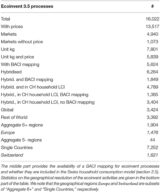
Table 1. The first part of the table shows the number of ecoinvent processes containing price information for their reference products.

2.3. BACI Trade Data

In this paper we aim to capture realistic price distributions based on commodity trade data. In particular, we use the BACI⁴ trade data base version HS12 2020 1 for the year 2012, which provides bilateral trade data on 5,199 commodities and 221 countries (Gaulier and Zignago, 2010). BACI is based on the United Nations (UN) Comtrade Database⁵ and offers a harmonised data set in which discrepancies in the raw data between exporter and importer reports are reconciled. The products are defined in the Harmonised System (HS) nomenclature, at the six digit level. The BACI trade flows are reported in Free Onboard (FOB) values, for which the Cost, Insurance, Freight (CIF) values declared by the importing country have been adjusted to reconcile them with their mirror flows reported by the exporting country. All flows are, crucially, also provided in the physical units of metric-tons, see Gaulier and Zignago (2010) for details on the conversion from other units to metric-tons. Most importantly, the reports of physical flows allow us to obtain an average price for the trade flows of a given commodity between two countries. This average price is calculated by dividing the monetary flow value by the physical amount and then converted from USD to Euro using the annual average exchange rate for 2012 of 0.78 Euro/USD, obtained from Eurostat⁶.

2.3.1. Mapping BACI Flows to Ecoinvent Processes

In a first step to link ecoinvent products to BACI trade flows we use the concordance tables available at the UN statistics division⁷ to create a mapping between the HS12 BACI data and the ecoinvent reference products of each process which are given in the “central product classification” system, version CPC2.1. In order to avoid introducing any more uncertainty, we only consider ecoinvent products which are quantified in “kg” and that have a CPC2.1 code with at least the “class” defined (four digits). We then map the ecoinvent regions, including all unique “rest of world” (RoW) areas, to the 221 countries present in BACI. Both concordances are available in the github repository linked at the end of this document.

To obtain a price distribution for the reference product of an ecoinvent process, we use the volume weighted export price distribution of mapped commodities from all countries within the ecoinvent region. We note that while this excludes domestic trade flows (BACI only covers international trade), the assumption is that the international trading price distribution will also adequately capture the price variability in domestic markets, as BACI trade flows are given in Free Onboard Prices. For global processes all trade flows of the relevant commodities are present in the price distribution.

The median number of flows matched to an ecoinvent activity is 1,292. The number of flows mapped to an activity is a function of the number of BACI commodities mapped to the reference product (see Figure 1A) and the geographical resolution. The large (median) number of matched flows stems mainly from the fact that many of the ecoinvent processes are “global” or RoW processes, or from other large aggregate regions such as “Europe” (see Table 1). The large (median) number of flows associated with ecoinvent activities illustrates the many trading relations covered by each activity. Here, the authors want to point out though, that the actual number of trading relations will likely be much higher than the number of flows in BACI, as these cover only the total trading volumes between countries as a whole. The number of BACI/HS12 commodities mapped to the reference products of the ecoinvent processes is shown in Figure 1A. The first bar indicates that there are 1,771 ecoinvent processes whose reference product has a 1:1 match to a BACI commodity. The largest number of BACI commodities matched to a single reference product is 53, whereas the median is 4. The reason that multiple BACI commodities can be mapped to a reference product is the higher commodity resolution of BACI compared to reference products' CPC classification. In the mapping between BACI flows and ecoinvent processes, we rely on a classification (CPC) that does not fully capture the level of detail present in the ecoinvent database, e.g., a very particular alloy might be classified as broader category of alloys because a finer classification does not exist in the CPC and HS classification schemes. Certainly, this can lead to an incorrect (median) price estimate for this particular alloy, but it is reasonable to assume that the real price will be present in the price distribution for the activity's reference product. Moreover, the more specific the reference product is, the smaller the production volume will become compared to more generic products, therefore these cases will likely not have a strong impact on the statistical outcome of this study.

FIGURE 1

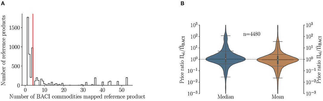
Figure 1. The distribution of the number of BACI (HS12) commodities matched to the reference products of ecoinvent activities (A). The vertical red line shows the median at four commodities per reference product. (B) Shows the distribution of the ratio of ecoinvent prices Π_ei and the median- (${\tilde{\Pi }}_{\text{BACI}}$) and mean (${\bar{\Pi }}_{\text{BACI}}$) price respectively from the BACI volume weighted price distribution Π_BACI. The horizontal lines in the violins indicated the 2.5, 16, 50, 84, and 97.5% quantiles. The long dashed horizontal line shows a ratio of 1. The number of reference products (n = 4,480) is smaller than the number of activities/reference products that have a BACI price (n = 5,624) because not all of these processes have an ecoinvent price.

A comparison of the prices in ecoinvent to the BACI median and mean prices is given in Figure 1B. Here both the median and the mean price refer to the median and mean of the volume weighted price distribution for each activity/reference product. Only 4,480 reference products were used in this comparison instead of all 5,624 that have a BACI price because for the remaining reference products ecoinvent does not provide a price. The horizontal lines in the violins indicate, from bottom to top, the 2.5, 16, 50, 84, and 97.5% quantiles. The median price ratios Π_ei/Π_BACI are 1.16 and 0.90 for the BACI median and mean prices, respectively. That the median BACI price is lower than the mean price is a natural consequence of the skewed nature of prices (they are “strictly” positive) and the sensitivity of the mean to outliers. Although there is a rather large spread in the ecoinvent/BACI price ratios, we see that the distributions are strongly peaked around 1:68% of BACI prices lie within a factor of 0.4–5.31 (median) and 0.25–2.66 (mean) of the ecoinvent price. This means that the hybrid footprints calculated using BACI prices will likely have very similar expectation values as the ones calculated using ecoinvent prices. Here, the expectation value refers to the fact that the BACI prices are treated as random variables, which leads to a range of possible hybrid footprint outcomes rather than a deterministic one.

Because of the statistical nature of this study and the high variability in trading relations, throughout this study we use the median rather than the mean, as the former metric is less sensitive to (extreme) outliers. In the Monte Carlo analysis, the median price is also the one sampled most frequently. Note that for this comparison of ecoinvent and BACI prices we applied an inflation correction⁸ of 1.16 to the “2005” ecoinvent prices in order to adjust them to our reference year 2012.

2.3.2. Sources of Price Variance

This paper analyses the effect of price variance on the uncertainty of environmental footprints in an hybrid-LCA analysis. It is therefore important to understand what drives this price variance, e.g., whether it originates in the limited trade data resolution, the geographical resolution of the processes, or can we identify other sources? To this end we calculate the median price variance of the reference products of the (hybridised) processes with BACI price data, divided in different subsets. The results of this are presented in Figure 2 as the relative Median Absolute Deviation (rMAD) of various subsets of the data. We use the rMAD as an estimate of the variability instead of the more commonly used coefficient of variation for the former's robustness against outliers. The subsets are organised in three groups: the first group divides the processes by their geographical resolution: Global, Rest of World, Aggregate regions with six or more countries, Aggregate regions with fewer than six countries, and single country processes. The second group divides the processes based on the level of detail in the CPC classification of the reference product and the uniqueness of the CPC-HS nomenclature matching. The subsets are: four CPC digits (class) available, five CPC digits (subclass) available, and a unique HS code mapping, which means only 1 HS code was mapped to the CPC code of the process' reference product). The third group divides processes into CPC sections (section 0 “Agriculture, forestry and fishery products,” section 1 “Ores and minerals; electricity, gas and water,” section 2 “Food products, beverages and tobaccos; textiles, apparel and leather products,” section 3 “Other transportable goods, except metal products, machinery and equipment,” and section 4 “Metal products, machinery and equipment”).

FIGURE 2

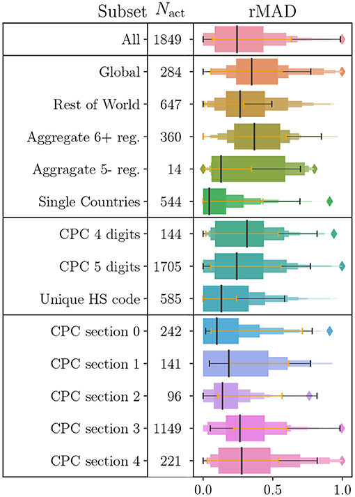
Figure 2. The statistical price variance of the reference products of processes with a BACI price distribution, given as the median price variability of the robust indicator relative Median Absolute Deviation (rMAD) for different subsets of processes hybridised with BACI price data. The subsets are divided into three groups: “regional resolution,” “CPC-HS mapping quality,” and “commodity type.” The orange and black horizontal errorbars indicate the 16–84% and the 2.5–97.5% quantiles, respectively.

We find that the geographical aggregation, the quality of the matching and the commodity type all have a strong impact on the price variance, with the respective lowest uncertainty subsets being consistent with each other within the 95% quantile range. The intersection of the “single country” and “unique HS code” subsets contains less than half the processes of each subset, a total of 243 processes. Although the “unique HS code” criteria ensures that the CPC code of the process' reference product holds the highest level of detail required for a 1–1 matching with a BACI (HS) commodity, it does not mean that this classification consists of homogeneous commodities. This, however, was judged to be the case for the majority of the cases by the authors, with 173 processes in the “unique HS code” coming from the Agriculture, forestry, and fishery (CPC section 0) subset, consisting of simple non-manufactured products. Moreover, 142 of the processes in the “CPC section 0” subset are “single country processes,” which is why it is perhaps not surprising that these processes show a low median uncertainty and a relatively small range compared to the other subsets.

2.4. Price Distribution for Hybridised Processes Without BACI Data

Not all hybridised processes in the life cycle inventory of the Swiss household consumption survey have mapped trade flows in BACI (see Table 1). We model the price uncertainty for the remaining processes as a lognormal distribution with a mean at the ecoinvent price and a shape parameter derived from the price variance in proxy data. To find proxy data, we categorise the remaining 3,390 processes with a non-zero production in the full life cycle inventory (see Table 2). For each category we estimate a coefficient of variation which we subsequently use to model lognormal price distributions. For the “electricity” category, we use the price variance across different consumption groups, based on volume of consumption, in the EU for the year 2012⁹. Since the majority of the processes in the “steam and hot water” category are “heat and power co-generation” processes, their price distribution is modelled using the same variance parameter as used for electricity. The variance in the freight category is derived from the variance in the crude oil prices of OECD countries between 2012 and 2013 (OECD, 2020). The remaining processes each get the median coefficient of variation from the processes that have a BACI mapping.

TABLE 2

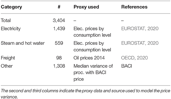
Table 2. Categorisation of the processes with non-zero production in the Swiss Household consumption final demand, but without matching BACI trade flows.

2.5. Functional Unit: Swiss Household Consumption

In order to assess the impact of the price variability on a hybrid-LCA consumption based footprint, we use the process LCA part of the model by Froemelt et al. (2018) of the Swiss household budget survey (HBS 2009–2011; Bundesamt für Statistik, 2013). The survey provides detailed information on the consumption of 9,734 households, which reported their daily expenditures and quantities of purchased goods for the period of 1 month. Additionally, periodic expenditures, service subscriptions, and extraordinary purchases and revenues were reported. Froemelt et al. (2018) used this 2009–2011 household budget survey to model and assess the environmental impacts of consumption behaviour, using ecoinvent, EXIOBASE, and AGRIBALYSE (Koch and Salou, 2016). Here we use the PLCA part of the model from Froemelt et al. (2018) to obtain a final demand vector for the average monthly consumption of a Swiss household. Since in this study we are interested in the effect of price uncertainty of the hybrid LCA footprint results, we only consider the consumption mapped to ecoinvent processes, which cover 61% of the total carbon footprint in 2011. We note that the consumption covered by AGRYBALYSE processes only accounted for <0.5% of the average household carbon footprint. Furthermore, for consistency with the other data sources used in this study, we scale this data with an inflation- and population-corrected GDP growth factor for “households and non-profit institutes serving households” of 1.6% to the year 2012, using data from the Swiss Statistical Office¹⁰. For further details of the Swiss household consumption model we refer the interested reader to Froemelt et al. (2018).

Although the complete model by Froemelt et al. (2018) falls into the “tiered hybrid” category as defined by Crawford et al. (2018), we note that as we only consider the PLCA part of the model by Froemelt et al. (2018), the hybridisation in this study only concerns the background, and the foreground system remains non-hybridised.

2.6. Monte Carlo Simulation

The main component of the integrated hybrid model is the upstream cut-off matrix C^u. The elements in C^u depend column-wise on the product prices of the hybridised LCA processes. To assess the impact of the price variability we use an adaptation of the open source hybridisation tool pyLCAIO (Agez et al., 2020) to create a cut-off matrix that is not “scaled” with the price vector. Such that:

$\begin{array}{ll}{C}_{\text{unscaled}}^u=\text{Corr}◦A^{\text{io}}(H◦\text{Geo}).& (3)\end{array}$

We then perform a Monte Carlo simulation by drawing prices from the price distributions of the relevant processes, defined as described in sections 2.3.1 and 2.4, to construct 10,000 realisations of the “scaled” C^u matrix. Although in reality commodity prices will be subject to correlations, i.e., the prices of steel based products will likely positively correlate with the market price for steel, market dynamics do not necessarily follow the same patterns, making such correlations a very complex problem to model. Without adequate data on possible price (anti-)correlations, this remains outside the scope of this work, and prices of the reference products are sampled independently.

3. Results

In this section we present the results of the Monte Carlo simulations on the effect of price uncertainty for the two double counting correction scenarios “STAM” and “binary.” We first present the results of a statistical uncertainty on the process level [for the midpoint indicator global warming potential (GWP) 100] before presenting the results for the consumption basket of the Swiss Household budget survey.

3.1. Process Level Uncertainty

Table 3 shows the median increase in the hybrid Carbon Footprint Intensity (CFI) over the pure PLCA CFI. The CFI is defined as the carbon footprint of 1 unit of the reference product of a process. Additionally, the median uncertainty range (2.5–97.5% quantiles) for both the full hybrid CFI as well as just the IO part (or truncation error correction) of the CFI are given. The table provides the results for both double counting correction strategies, and presents the results for different process groups. The first column gives the considered process group, where (A) are all processes in the ecoinvent LCI, (B) are the hybridised processes with BACI price data, (C) are the hybridised processes without BACI price data, described in section 2.4, (D) are all hybridised processes, and (E) are all non-hybridised processes. Although the latter category of processes do not get a direct contribution from the MRIO background, they still see an increase in their hybrid CFI through the hybridised processes in their supply chain.

TABLE 3

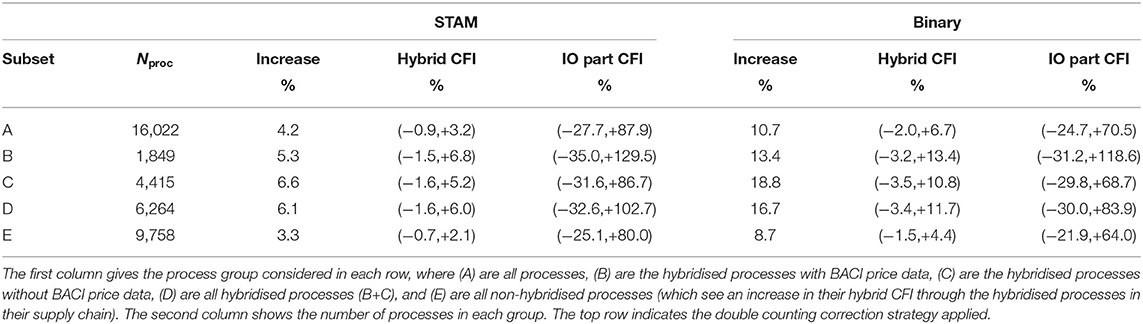
Table 3. The increase and uncertainty in the statistical hybrid carbon footprint intensity (CFI) at the process level, presented as the median GWP100 percentual increase over the pure PLCA CFI and the variability within the 2.5 and 97.5% quantiles for both the total hybrid CFI and just the IO- (or hybrid-) part.

We find a median relative increase in the CFIs of 6.1 and 16.7% for all hybridised processes (process group D) in the “STAM” and “binary” double counting correction scenarios, respectively. Furthermore, the effect of the price variance on the hybrid- or IO part of the process' CFIs is high with the median uncertainty in the CFIs for all hybridised processes (group D) being (−33, +103%), resulting in an overall CFI uncertainty of (−2, +6%) for the same group in the STAM double counting correction scenario. Using the binary double counting correction, this becomes (−30, +84%) and (−4, +12%), respectively. Additionally, we find the impact of hybridisation on the CFI uncertainty of non-hybridised processes to be (−1, +2%) and (−2, +4%) in both double counting correction strategies.

3.2. Footprint Uncertainty for the Swiss Household Consumption Basket

The footprint results (for the midpoint indicator global warming potential GWP100) of the average Swiss household consumption basket, for both the “STAM” and “binary” scenarios are presented in Tables 4, 5, respectively. The results are given for different subsets of the processes to enable the identification of the impact of the price uncertainty on the total hybrid footprint (Γ), on the hybridised processes that have BACI price data (Δ), the hybridised processes without BACI price data and modelled as described in section 2.4 (Θ), and all hybridised processes (Λ). The percentage columns show the percentage points of the footprint stemming from the hybridisation, or input-output part of the model, compared to the footprint covered by the process LCA part of the model. We note however, that although the total number of processes in the life cycle inventory is higher for subset Γ than for subset Λ, leading to a higher PLCA footprint, the number of hybridised processes is the same in both and equal to the total number of processes in subset Λ: 4,789.

TABLE 4

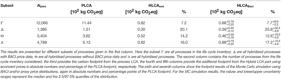
Table 4. The footprint results (GWP100) of the consumption basket of an average Swiss Household using the “STAM” double counting correction strategy.

TABLE 5

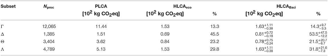
Table 5. As Table 4, but for the “binary” double counting correction scenario.

Figures 3, 4 show the Monte Carlo result distributions of the relative increase of the hybrid footprint compared to the PLCA footprint. The left and right panels show the distributions of the subsets Γ and Δ for the “STAM” and “binary” double counting correction strategies, respectively. The vertical lines indicate 2.5, 16, 50% (median), 84 and 97.5% quantiles as well as the mean and the footprint using ecoinvent prices without uncertainty. We find that although the distributions for both double counting correction scenarios are wide, showing a long tail toward the positive side, the distributions do show a strong peak around median and mean of the distributions. The skew of the distribution is a direct consequence of the skewed nature of prices (Π_i > 0).

FIGURE 3

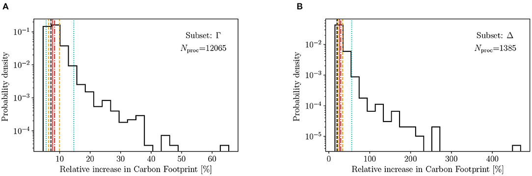
Figure 3. The uncertainty distribution of the relative increase in carbon footprint (GWP100) due to hybridisation, using the STAM double counting correction method, for the overall hybrid footprint (A) and the 1,385 processes with a price sampling variance from the BACI trade data based on produced commodity and region (B). The dotted (cyan) and dashed (orange) vertical lines indicate the 95 and 68% confidence intervals, the red solid and dashed dotted lines show the median and mean of the distribution. The black dashed line indicates the impact using the ecoinvent prices.

FIGURE 4

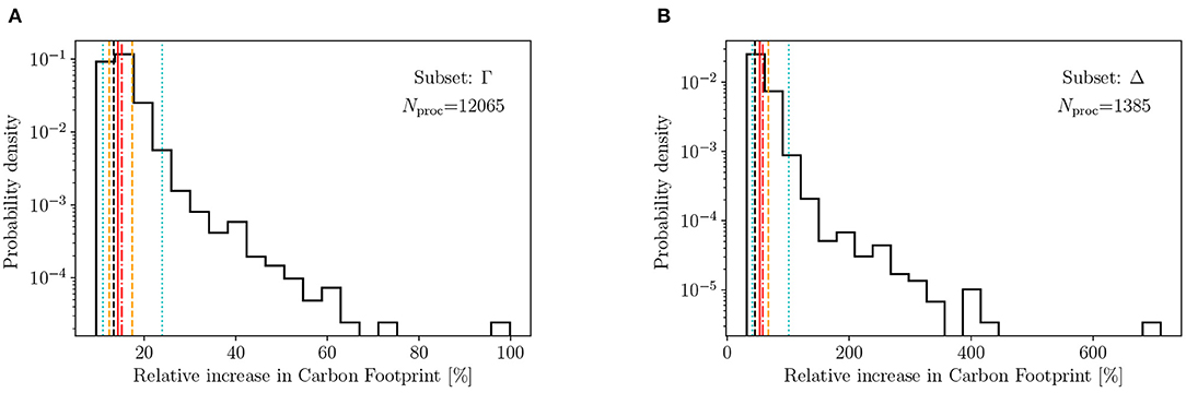
Figure 4. The uncertainty distribution of the relative increase in carbon footprint (GWP100) due to hybridisation, using the “binary” double counting correction method, for the overall hybrid footprint (A) and the 1,385 processes with a price sampling variance from the BACI trade data based on produced commodity and region (B). The dotted (cyan) and dashed (orange) vertical lines indicate the 95% and 68% confidence intervals, the red solid and dashed dotted lines show the median and mean of the distribution. The black dashed line indicates the impact using the ecoinvent prices.

Although using the “STAM” double counting correction, the hybridisation accounts only for 7.7% of the PLCA footprint for the full LCI, using the “binary” double counting correction this goes up to 14.3% for the full LCI (subset Γ). If we only consider the hybridised processes that have a BACI price, this becomes 25.8 and 53.5%, respectively (subset Δ). Moreover, the relative uncertainty of this hybrid part of the footprint (i.e., the truncation error correction) is (−28, +90%) and (−23, +68%) in the “STAM” and “binary” case respectively for the 2.5 and 97.5% quantiles. For subset Δ this becomes, in the same order (−26, +117%) and (−23, +89%).

4. Discussion

Here we discuss these results in the context of the findings of other studies and go into the implications and limitations of this study.

The level of truncation error estimates or the relative increase of hybrid LCA footprints (-intensities) over process LCA vary in literature. Most of these studies consider either a specific case study (Perkins and Suh, 2019), or look at the carbon footprint intensities (CFIs) of individual processes (Yu and Wiedmann, 2018; Agez et al., 2020), or average truncation errors of processes in different industry sectors (Ward et al., 2018). In this study we considered both the median process level uncertainty and a consumption basket of an average Swiss household. We note however, that for this analysis we focus only on the process- or hybrid LCA part of the consumption basket that is covered by ecoinvent and leave out the part that is modelled solely on EXIOBASE and AGRIBALYSE. The different methodologies used in literature to study the truncation errors in PLCA make it difficult to compare the various results one to one. Our process level CFIs are most comparable to Agez et al. (2020) (STAM double counting correction) and Yu and Wiedmann (2018) (binary double counting correction) as both these studies look at the hybridisation of a whole database. However, to provide a better context and highlight the complexity of the issue of truncation errors we discuss below how the results of this study fit into the wider literature.

At the process level, we find that the CFI of hybridised processes (subset D, Table 3) sees a median increase of 6.1 and 16.7% in the “STAM” and “binary” double counting correction scenarios, respectively. This is below most estimates of the truncation error in literature on a process basis: e.g., Ward et al. (2018) find average sector truncation errors between 7 and 76% for different industry sectors and estimation methods, Yu and Wiedmann (2018) find an average increase between 21 and 32% in their different double counting correction scenarios, and Perkins and Suh (2019) find a relative increase of 38% compared to a pure PLCA in their case study of a jacket. In the case of the household consumption basket, the relative increase of the HLCA compared to the PLCA of the overall footprint (subset Γ), is also modest, though not insignificant, being $7.7_{-2.2}^{+6.9}\%$ in the “STAM” scenario, and increasing to $14.3_{-3.3}^{+9.7}\%$ in the “binary” case. However, out of the 12,065 processes in the total life cycle inventory, only 4,789 were hybridised. If we consider these processes only (subset Λ), we find a relative increase of $17.2_{-4.9}^{+15.5}$ and $31.8_{-7.3}^{+21.6}$ in the “STAM” and “binary” scenarios respectively, which is still below the aforementioned studies, but consistent within the 95% confidence interval of our results. We note here that (Agez et al., 2020), using the “STAM” double counting correction method, find a relative carbon footprint increase per process with a median of 7% and an average of 14%, but a large spread with processes displaying up to 1,100% relative increase. The slightly lower median increase on process level CFIs in this study can be explained by the slightly lower median prices for the reference products in BACI compared to the ecoinvent prices (see Figure 1B).

Looking at the relative uncertainty due to price variances, Yu and Wiedmann (2018) find relative uncertainties for the individual CFIs between −31 and +33% in their different double counting correction strategies, with average CFI variations between −4.7 tp +5.1% and −3.3 to +3.2% for the two different double counting correction strategies. These results are based on normally distributed price uncertainties with 30% relative standard deviation. We find a median hybrid CFI uncertainty of (−1.6, +6.0%) and (−3.4, +11.7%) for the “STAM” and “binary” scenarios, respectively. We see that where the uncertainties of Yu and Wiedmann (2018) are relatively symmetric as a natural result of their symmetric price uncertainties, we find highly positively skewed uncertainty ranges, with the lower range being smaller than found by Yu and Wiedmann (2018) and the upper range well above the results of that study. Considering the consumption basket case we find a total hybrid footprint uncertainty of (subset Γ) of (−2.0, +6.4%) and (−2.9, +8.5%) (in the 95% confidence interval) for “STAM” and “binary” scenarios, respectively. Focusing again only on the hybridised processes (subset Λ), we find a variance of the hybrid carbon footprint of (−4.2, +13.2%) and (−5.6, +16.4%). Considering only the processes for which BACI price data are available (subset Δ), we find the uncertainty increases even further to (−5.2, +22.9%) and (−7.6, +30.5%) for the “STAM” and “binary” scenarios, respectively. These relative uncertainties of the hybrid carbon footprints are in the higher end of the range in the findings of Yu and Wiedmann (2018).

Placing our findings in the light of the accuracy vs precision debate (Perkins and Suh, 2019, and references therein), we see that at an “accuracy” (truncation-) correction of 17 and 32%, the uncertainty associated with this correction is (−28, +90%) and (−23%, +68%) relative to the magnitude of the correction, for all hybridised processes in our consumption basket (subset Λ) in the “STAM” and “binary” scenarios, respectively. This equates to an overall precision loss (added total footprint uncertainty) of (−4, +13%) and (−6, +16%). On the total consumption basket (subset Γ) we find an accuracy correction with a magnitude of 8, 14% with the same relative uncertainty as subset Λ and a footprint precision loss of (−2, +6%) and (−3, +8%).

We have to keep in mind that this is a statistical work, based on statistical trading data, but as Yu and Wiedmann (2018) point out, finding accurate prices, and price distributions for individual commodities and services is a highly time and effort consuming task which makes it at this point an unrealistic option for a database-wide hybridisation. A statistical approach such as taken in this study might have its shortcomings, e.g., the available commodity categories in trade databases such as BACI might be too aggregated to accurately capture the prices of individual commodities that do not represent the “average” product within the commodity category. However, the diversity of trading relations between different countries will likely still capture much of the variance accurately. Moreover, we have shown that the geographical aggregation of the ecoinvent processes is responsible for a significant part of the price variance in low geographical resolution (e.g., global or rest-of-world) processes. This indicates that regionalisation of process inventory databases (Mutel and Hellweg, 2009) has the added benefit of smaller price variation of the reference products, leading to more accurate hybrid CFIs.

The results of this study show that price variation can lead to significant uncertainty in hybrid footprints, although the positive skew of this uncertainty means that the probability of underestimating the truncation error correction is larger than the probability of overestimating the resulting hybrid footprint. This implies that precision loss (added uncertainty) due to price variance in the hybridisation process, will likely not weigh up to the accuracy gain (truncation error correction). As pointed out above, finding accurate price data (including information on variance and ranges) for all reference products of a databases is an unrealistic undertaking for each individual hybrid LCA study. So until process inventory databases publish information on the price variance, practitioners have to rely on statistical price data such as presented in this study for background processes and may put extra effort into finding accurate price ranges for the foreground processes of the study. As a first step toward price variance inclusion within process inventories, a pedigree matrix approach as used in ecoinvent for technosphere exchanges (Muller et al., 2016) could be developed for price data, particularly given the strong dependence of the price variance on geographical resolution and product type as we found in section 2.3.2.

In section 2.2, we discussed that prices of products in co-production are used for economic allocation purposes. This of course means that if these prices are not deterministic but also random variables, this will directly impact allocation of the inputs to co-products and hence all supply chains containing any of these co-products. Because of the high interconnectivity (Moreno Ruiz et al., 2016) in practice this means that most processes are affected. The authors are not aware of published studies looking at the effect of price variance on economic allocation in process inventory databases and the resulting process CFIs.

In this paper we presented the carbon footprint (intensity) results to illustrate the impact price uncertainty or variance has on hybrid LCA footprints. We note however, that although the actual footprint uncertainty ranges for different impact categories might change due to different IO industries having varying impact levels for different impact indicators, the impact of the price uncertainty remains the same. That also leads us to the fact that in this study we only look at the uncertainty arising from price variance. We do not consider uncertainty within the LCA supply chains, nor in the biosphere flows and impact categories. Furthermore, uncertainty remains due to aggregation error of IO sector compared to the individual processes of the PLCA database (Yu and Wiedmann, 2018; Perkins and Suh, 2019), which will depend on the sectoral and regional resolution of the (multi-regional) IO table. To include this fully, one would need to capture the variance in intraindustry supply chains as well as the intraindustry stressor variation (emission/euro) (Majeau-Bettez et al., 2011). Another important source of uncertainty in integrated and tiered hybrid models is the issue of double counting (Agez et al., 2019). We find the difference in truncation error correction between the more conservative STAM double counting correction method and the less strict “binary” approach to be around a factor of almost 2 for all processes in the Swiss consumption case (subset Γ). This indicates that the uncertainty arising from the double counting correction is another substantial source of uncertainty in hybrid LCA and needs to be taken into consideration. Finally, as discussed in section 2.6, we also do not consider possible correlations between the prices of different products. Although the presence of correlations would reduce the uncertainty, they are subject to various influences acting on different time scales. The complexity of this problem puts it outside the scope of this study.

In conclusion, we present the first data driven analysis of the effect on price uncertainty on process carbon footprint intensities and illustrate the magnitude of the resulting uncertainty on a statistical footprint study of Swiss household consumption. We find that although the relative increase of hybridisation is small to moderate in the consumption study (8–14%) for the two different double counting correction methods, the uncertainty of this contribution to the footprint due to price variability is very high (−28 to +90%) and asymmetric, with the uncertainty ranges being (strongly) positively skewed. This highlights the need of accurate prices and price distributions in hybrid LCA studies.

Data Availability Statement

The python code and classification mappings used to generate the results for this study can be found in the github repository (https://github.com/jakobsarthur/Price_Uncertainty_HLCA). The full Monte Carlo simulation results will be send upon request.

Author's Note

The merit of including input-output data to improve the accuracy of process life cycle analyses (LCA) in so called hybrid-LCA is an active area of research. Consensus seems to exist that the added uncertainty due to the low resolution of the input-output data, is smaller than the accuracy gain. However, the uncertainty due to price variance of the commodities in the process life cycle inventory has so far only been assessed using non-process-specific theoretical price uncertainties. This paper presents the first study assessing the effect of process-specific commodity price variance on hybrid footprints. Commodity prices and their variances are estimated, using detailed trade data from the United Nations statistical department. We find that the geographical resolution of process data is a main driver of commodity price variation. We show that price variability leads to high and positively skewed uncertainty of the hybrid footprints. This work is the first data driven analysis of the effect of price variance in hybrid footprints, and highlights the importance of using process-specific price distributions when performing hybrid-LCA.

Author Contributions

AJ: analysis, results, figures, and text. AJ and SS: concept. AJ, SP, and SS: editing. SP: supervision. All authors contributed to the article and approved the submitted version.

Funding

AJ was funded through- and conducted this research as part of the project Open Assessment of Swiss Economy and Society, funded by the Swiss National Science Foundation grant number 407340_172445 as part of the National Research Program Sustainable Economy: resource-friendly, future-oriented, innovative (NRP 73). SS received funding from the Eva Mayr-Stihl foundation.

Conflict of Interest

The authors declare that the research was conducted in the absence of any commercial or financial relationships that could be construed as a potential conflict of interest.

Acknowledgments

The authors are very grateful for the support of Aleksandra Kim and Andreas Frömelt for their help with the Swiss consumption model, Chris Mutel for his insightful and inspiring discussions, Guillaume Bourgault for the extensive exchanges on the ecoinvent data, and Carsten Dormann for his input regarding the statistical analysis and providing feedback on the manuscript. The authors would also like to thank Maxime Agez, for his quick and helpful responses to questions regarding the use of pylcaio. Furthermore, the authors would like to thank, in no particular order, Stefanie Klose and Kavya Madhu for the many discussions and support. Last the authors would like to thank Christina Bartz and Merlijn Jakobs for their support and for proof reading this manuscript.

Footnotes

1. ^http://www.auslci.com.au

2. ^http://ielab.info

3. ^https://github.com/MaximeAgez/pylcaio

4. ^http://www.cepii.fr/CEPII/en/bdd_modele/presentation.asp?id=37

5. ^https://comtrade.un.org/

6. ^https://ec.europa.eu/eurostat/databrowser/bookmark/bc107428-d077-4a9a-86a5-a4f045cf63e9?lang=en (accessed November 27, 2020).

7. ^https://unstats.un.org/unsd/classifications/econ/

8. ^https://www.inflationtool.com/euro?amount=100&year1=2005&year2=2014 (accessed November 27, 2020).

9. ^https://ec.europa.eu/eurostat/databrowser/view/NRG_PC_205__custom_509016/default/table?lang=en (accessed January 28, 2021).

10. ^GDP: https://www.bfs.admin.ch/bfs/en/home/statistics/national-economy/national-accounts/gross-domestic-product.assetdetail.14347475.html (accessed January 28, 2021).Population: https://www.bfs.admin.ch/bfs/en/home/statistics/population.assetdetail.14367975.html (accessed January 28, 2021).

References

Agez, M., Majeau-Bettez, G., Margni, M., Strømman, A. H., and Samson, R. (2019). Lifting the veil on the correction of double counting incidents in hybrid life cycle assessment. J. Indus. Ecol. 24, 517–533. doi: 10.1111/jiec.12945

CrossRef Full Text | Google Scholar

Agez, M., Wood, R., Margni, M., Strømman, A. H., Samson, R., and Majeau-Bettez, G. (2020). Hybridization of complete PLCA and MRIO databases for a comprehensive product system coverage. J. Indus. Ecol. 24, 774–790. doi: 10.1111/jiec.12979

CrossRef Full Text | Google Scholar

Bontinck, P. A., Crawford, R. H., and Stephan, A. (2017). Improving the uptake of hybrid life cycle assessment in the construction industry. Proc. Eng. 196, 822–829. doi: 10.1016/j.proeng.2017.08.013

CrossRef Full Text | Google Scholar

Bruckner, M., Wood, R., Moran, D., Kuschnig, N., Wieland, H., Maus, V., et al. (2019). FABIO-the construction of the food and agriculture biomass input-output model. Environ. Sci. Technol. 53, 11302–11312. doi: 10.1021/acs.est.9b03554

PubMed Abstract | CrossRef Full Text | Google Scholar

Bundesamt für Statistik (2013). Haushaltsbudgeterhebung 2011. Neuchâtel: Bundesamt für Statistik (BFS).

Crawford, R. H., Bontinck, P.-A., Stephan, A., Wiedmann, T., and Yu, M. (2018). Hybrid life cycle inventory methods-a review. J. Clean. Prod. 172, 1273–1288. doi: 10.1016/j.jclepro.2017.10.176

CrossRef Full Text | Google Scholar

Crawford, R. H., Bontincka, P.-A., Stephana, A., and Wiedmann, T. (2017). Towards an automated approach for compiling hybrid life cycle inventories. Proc. Eng. 180, 157–166. doi: 10.1016/j.proeng.2017.04.175

CrossRef Full Text | Google Scholar

EUROSTAT (2020). Electricity Prices for Non-Household Consumers - Bi-Annual Data (From 2007 Onwards). EUROSTAT.

Froemelt, A., Dürrenmatt, D. J., and Hellweg, S. (2018). Using data mining to assess environmental impacts of household consumption behaviors. Environ. Sci. Technol. 15, 8467–8478. doi: 10.1021/acs.est.8b01452

PubMed Abstract | CrossRef Full Text | Google Scholar

Gaulier, G., and Zignago, S. (2010). BACI: International Trade Database at the Product-Level (the 1994-2007 Version). CEPII Working Paper 2010–23. doi: 10.2139/ssrn.1994500

CrossRef Full Text | Google Scholar

Heijungs, R., and Suh, S. (2002). The Computational Structure of Life Cycle Assessment. Dordrecht: Springer-Verlag. doi: 10.1007/978-94-015-9900-9

CrossRef Full Text | Google Scholar

Islam, S., Ponnambalam, S. G., and Lam, H. L. (2016). Review on life cycle inventory: methods, examples and applications. J. Clean. Prod. 136, 266–278. doi: 10.1016/j.jclepro.2016.05.144

CrossRef Full Text | Google Scholar

Junnila, S. I. (2006). Empirical comparison of process and economic input-output life cycle assessment in service industries. Environ. Sci. Technol. 40, 7070–7076. doi: 10.1021/es0611902

PubMed Abstract | CrossRef Full Text | Google Scholar

Kalbar, P. P., Birkved, M., Kabins, S., and Nygaard, S. E. (2016). Personal metabolism (PM) coupled with life cycle assessment (LCA) model: Danish case study. Environ. Int. 91, 168–179. doi: 10.1016/j.envint.2016.02.032

PubMed Abstract | CrossRef Full Text | Google Scholar

Koch, P., and Salou, T. (2016). AGRIBALYSE Rapport Metholodogique - Version 1.3. Ademe.

Google Scholar

Larsen, H. N., and Hertwich, E. G. (2009). The case for consumption-based accounting of greenhouse gas emissions to promote local climate action. Environ. Sci. Policy 12, 791–798. doi: 10.1016/j.envsci.2009.07.010

CrossRef Full Text | Google Scholar

Lenzen, M. (2001). Errors in conventional and input-output-based life-cycle inventories. J. Indus. Ecol. 4, 127–148. doi: 10.1162/10881980052541981

CrossRef Full Text | Google Scholar

Lenzen, M. (2009). Dealing with double-counting in tiered hybrid life-cycle inventories: a few comments. J. Clean. Prod. 17, 1382–1384. doi: 10.1016/j.jclepro.2009.03.005

CrossRef Full Text | Google Scholar

Lenzen, M., and Crawford, R. (2009). The path exchange method for hybrid LCA. Environ. Sci. Technol. 43, 8251–8256. doi: 10.1021/es902090z

PubMed Abstract | CrossRef Full Text | Google Scholar

Lin, J., Liu, Y., Meng, F., Cui, S., and Xu, L. (2013). Using hybrid method to evaluate carbon footprint of Xiamen City, China. Energy Pol. 58, 220–227. doi: 10.1016/j.enpol.2013.03.007

CrossRef Full Text | Google Scholar

Majeau-Bettez, G., Strømman, A. H., and Hertwich, E. G. (2011). Evaluation of process- and input-output-based life cycle inventory data with regard to truncation and aggregation issues. Environ. Sci. Technol. 45, 10170–10177. doi: 10.1021/es201308x

PubMed Abstract | CrossRef Full Text | Google Scholar

Merciai, S., and Schmidt, J. (2018). Methodology for the construction of global multi-regional hybrid supply and use tables for the EXIOBASE v3 database. J. Indus. Ecol. 22, 516–531. doi: 10.1111/jiec.12713

CrossRef Full Text

Moreno Ruiz, E., Lévová, T., Reinhard, J., Valsasina, L., Bourgault, G., and Wernet, G. (2016). Documentation of Changes Implemented in Ecoinvent Data 3.1. Zurich: Ecoinvent. Technical report. Ecoinvent.

Google Scholar

Muller, S., Lesage, P., Ciroth, A., Mutel, C., Weidema, B. P., and Samson, R. (2016). The application of the pedigree approach to the distributions foreseen in ecoinvent v3. Int. J. Life Cycle Assess. 21, 1327–1337. doi: 10.1007/s11367-014-0759-5

CrossRef Full Text | Google Scholar

Mutel, C. L., and Hellweg, S. (2009). Regionalized life cycle assessment: computational methodology and application to inventory databases. Environ. Sci. Technol. 43, 5797–5803. doi: 10.1021/es803002j

PubMed Abstract | CrossRef Full Text | Google Scholar

OECD (2020). Crude Oil Import Prices (Indicator). OECD (accessed January 28, 2021).

Perkins, J., and Suh, S. (2019). Uncertainty implications of hybrid approach in LCA: precision versus accuracy. Environ. Sci. Technol. 53, 3681–3688. doi: 10.1021/acs.est.9b00084

PubMed Abstract | CrossRef Full Text | Google Scholar

Peters, G. P., and Hertwich, E. G. (2006). A comment on "Functions, commodities and environmental impacts in an ecological-economic model". Ecol. Econ. 59, 1–6. doi: 10.1016/j.ecolecon.2005.08.008

CrossRef Full Text | Google Scholar

Pomponi, F., and Lenzen, M. (2018). Hybrid life cycle assessment (LCA) will likely yield more accurate results than process-based LCA. J. Clean. Prod. 176, 210–215. doi: 10.1016/j.jclepro.2017.12.119

CrossRef Full Text | Google Scholar

Roos, S., and Zamani, P. (2015). Environmental Assessment of Swedish Fashion Consumption. Five Garments – Sustainable Futures. Approved as an external report from Mistra Future Fashion 15th of June 2015, Deliverable No: D2.6. Mistra Future Fashion Consortium.

Google Scholar

Sala, S., and Castellani, V. (2019). The consumer footprint: monitoring sustainable development goal 12 with process-based life cycle assessment. J. Clean. Prod. 240:118050. doi: 10.1016/j.jclepro.2019.118050

PubMed Abstract | CrossRef Full Text | Google Scholar

Stadler, K., Wood, R., Bulavskaya, T., Södersten, C.-J., Simas, M., Schmidt, S., et al. (2018). EXIOBASE 3: developing a time series of detailed environmentally extended multi-regional input-output tables. J. Indus. Ecol. 22, 502–515. doi: 10.1111/jiec.12715

CrossRef Full Text | Google Scholar

Stephan, A., Crawford, R. H., and Bontinck, P. A. (2019). A model for streamlining and automating path exchange hybrid life cycle assessment. Int. J. Life Cycle Assess. 24, 237–252. doi: 10.1007/s11367-018-1521-1

CrossRef Full Text | Google Scholar

Steubing, B., Wernet, G., Reinhard, J., Bauer, C., and Moreno-Ruiz, E. (2016). The ecoinvent database version 3 (part II): analyzing LCA results and comparison to version 2. Int. J. Life Cycle Assess. 21, 1269–1281. doi: 10.1007/s11367-016-1109-6

CrossRef Full Text | Google Scholar

Suh, S. (2004). Functions, commodities and environmental impacts in an ecological-economic model. Ecol. Econ. 48, 451–467. doi: 10.1016/j.ecolecon.2003.10.013

CrossRef Full Text | Google Scholar

Suh, S. (2006). Reply: downstream cut-offs in integrated hybrid life-cycle assessment. Ecol. Econ. 59, 7–12. doi: 10.1016/j.ecolecon.2005.07.036

CrossRef Full Text | Google Scholar

Suh, S., and Huppes, G. (2005). Methods for life cycle inventory of a product. J. Clean. Prod. 13, 687–697. doi: 10.1016/j.jclepro.2003.04.001

CrossRef Full Text | Google Scholar

Suh, S., Lenzen, M., Treloar, G. J., Hondo, H., Horvath, A., Huppes, G., et al. (2004). System boundary selection in life-cycle inventories using hybrid approaches. Environ. Sci. Technol. 38, 657–664. doi: 10.1021/es0263745

PubMed Abstract | CrossRef Full Text | Google Scholar

Towa, E., Zeller, V., Merciai, S., Schmidt, J., and Achten, W. M. (2020). Toward the development of subnational hybrid input-output tables in a multiregional framework. J. Indus. Ecol. 1–19. doi: 10.1111/jiec.13085

CrossRef Full Text | Google Scholar

Treloar, G. J. (1997). Extracting embodied energy paths from input-output tables: towards an input-output- based hybrid energy analysis method based hybrid energy analysis method. Econ. Syst. Res. 9, 375–391. doi: 10.1080/09535319700000032

CrossRef Full Text | Google Scholar

Treloar, G. J., Love, P. E., Faniran, O. O., and Iyer-Raniga, U. (2000). A hybrid life cycle assessment method for construction. Constr. Manage. Econ. 18, 5–9. doi: 10.1080/014461900370898

CrossRef Full Text | Google Scholar

Ward, H., Wenz, L., Steckel, J. C., and Minx, J. C. (2018). Truncation error estimates in process life cycle assessment using input-output analysis. J. Indus. Ecol. 22, 1080–1091. doi: 10.1111/jiec.12655

CrossRef Full Text | Google Scholar

Wernet, G., Bauer, C., Steubing, B., Reinhard, J., Moreno-Ruiz, E., and Weidema, B. (2016). The ecoinvent database version 3 (part I): overview and methodology. Int. J. Life Cycle Assess. 21, 1218–1230. doi: 10.1007/s11367-016-1087-8

CrossRef Full Text | Google Scholar

Yang, Y., Heijungs, R., and Miguel, B. (2017). Hybrid life cycle assessment (LCA) does not necessarily yield more accurate results than process-based LCA. J. Clean. Prod. 150, 237–242. doi: 10.1016/j.jclepro.2017.03.006

CrossRef Full Text | Google Scholar

Yu, M., and Wiedmann, T. (2018). Implementing hybrid LCA routines in an input-output virtual laboratory. J. Econ. Struct. 7:33. doi: 10.1186/s40008-018-0131-1

CrossRef Full Text | Google Scholar