An investigation of phase change induced Marangoni-dominated flow patterns using the Constrained Vapor Bubble data from ISS experiments

Kinetic models of liquid-vapor phase change often implicitly assume that the interface is in equilibrium. This equilibrium assumption can be justified for large flat interfaces far from the source of thermal energy, but it breaks down when the liquid surface is near a solid wall, or there is significant interface curvature. The Constrained Vapor Bubble (CVB) experiments conducted on the International Space Station (ISS) provide a unique opportunity to probe this common assumption and also provide unique data and insight into phase change-driven flow physics. The CVB experiment consists of a quartz cuvette partially filled with pentane such that a vapor bubble is formed at the center. The setup is heated and cooled at opposite ends, resulting in simultaneous evaporation and condensation. CVB data from the NASA Physical Science Informatics (PSI) database was used to reconstruct the entire 3D interface shape using interferometric image analysis and obtain an estimate of the net heat input to the bubble. The reconstructed interface shape is used to develop a liquid-only CFD model embedded with a custom-built “active surface” method that sets a variable interfacial temperature/phase change flux boundary condition. Phase change flux varies in both the axial and transverse directions, leading to a small (∼1 K) but discernible temperature variation along the liquid-vapor interface. The positive phase change flux near the heater end (denoting evaporation) gradually reduces and becomes negative near the cooler end (denoting condensation), resulting in an axial bulk flow of liquid from the cold to the hot end. There is also a higher flux in the thin film as opposed to the thick film, resulting in a transverse bulk flow. However, the interfacial temperature gradients along both axial and transverse directions induce a separate thermocapillary flow in a direction opposite to the bulk flows, leading to complex “wavy” flows with recirculation. A qualitative analysis of the flow pattern is presented in this paper and correlated with optical signatures from experimental images.

1 Introduction

Phase change is ubiquitous in nature and is widely used in several engineering applications. Although phase change is an inherently non-equilibrium interfacial transport phenomenon, it is common to model it in an equilibrium framework since the departure from equilibrium is minimal. This approximation finds its roots in diffusion-limited evaporation, where resistance to diffusion of the evaporated species in a quiescent gas typically dominates over interfacial transport resistance between the liquid and vapor. In such a case, the vapor close to the liquid surface is typically assumed to be at an equilibrium saturation condition. This reduces the liquid-vapor interface to a uniform isothermal surface. When interfacial resistance is dominant and/or there are no non-condensable gases in the vapor, equilibrium-based diffusion-limited models are no longer appropriate. In such cases, classical kinetic theory has been used to model liquid-vapor interface transport for over a century.

1.1 Kinetic theory of phase change

The rate at which liquid or vapor molecules pass through an arbitrary plane can be modeled using the Maxwell-Boltzmann distribution. When applied to the liquid-vapor interface, this approach allows for the net phase change rate to be modeled as the algebraic difference of the evaporation and condensation rates (Hertz, 1882; Knudsen, 1915). Several versions of kinetic models exist; the most widely accepted model was developed by Schrage (Schrage, 1953),

${\dot{m}}^{″}=\frac{2\alpha }{2-\alpha }\sqrt{\frac{m}{2\pi k_B}}\left[\frac{P_l}{\sqrt{T_i}}-\frac{P_v}{\sqrt{T_v}}\right](1)$

where m is the mass of a molecule, k_B is Boltzmann constant, P_l and P_v are liquid and vapor pressures near the liquid-vapor interface, T_i is the interfacial temperature, T_v is the vapor temperature, and α is the accommodation coefficient. Solving Eq. 1 is non-trivial since α is not typically known and T_i is difficult to measure experimentally. It may be simpler to assume T_i = T_v based on equilibrium arguments, but experimental investigations have shown a significant difference in liquid and vapor temperature during phase change, suggesting that T_v ≠ T_i (Fang and Ward, 1999; Ward and Stanga, 2001; Badam et al., 2007; Bellur et al., 2023).

1.2 Non-uniform phase change at curved interfaces

Equation 1 was developed for planar interfaces. Curvature and wetting dynamics have been shown to significantly affect the rate of phase change. Figure 1 shows the regions of interest along the evaporating meniscus of a wetting liquid. In the bulk region, where the film thickness is in the order of millimeters, capillary pressure caused by the surface tension and interface curvature dominates. This region is often characterized by a constant interface curvature. In the transition film (also called the thin-film) region, the thickness reduces to the micrometer range, along with a non-monotonically changing interface curvature. The reduction in film thickness enables a shorter conduction path resulting in an increase in phase change rate (Bellur et al., 2020; Lakew et al., 2023). The film thickness further reduces to nano-scale in the adsorbed film region, where the local physics is dominated by intermolecular forces commonly modeled as a disjoining pressure (net pressure reduction). In the adsorbed film, the disjoining pressure suppresses evaporation greatly and, in an equilibrium setting, can result in a non-evaporating film of constant thickness (Bellur et al., 2023; Lakew et al., 2023).

FIGURE 1

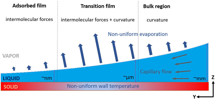
FIGURE 1. Region of the evaporating film of a wetting liquid. Heat is conducted from the solid wall to the liquid-vapor interface, where it contributes to phase change. The bulk region is dominated by the effects of curvature, and the adsorbed film is dominated by intermolecular forces between the solid wall and vapor molecules. The transition film region experiences a combination of these forces. Blue arrows represent evaporation flux, which peaks in the transition film region.

The thermal-fluid physics in transition film region is influenced by a combination of both disjoining pressure and capillary pressure (DasGupta et al., 1993; Ball, 2012). The net effect due to the interplay of anisotropies in local stress and heat transfer is a non-uniform evaporation flux that generally has a peak in the transition film (Bellur et al., 2020). For non-polar, wetting liquids, 60%–90% of the evaporation occurs in the transition film region close to the wall (Derjaguin et al., 1965; Potash and Wayner, 1972; Holm and Goplen, 1979; DasGupta et al., 1994; Wee et al., 2006; Plawsky et al., 2008; Fritz, 2012). The non-uniform evaporation results in a non-uniform temperature distribution making interfacial temperature, T_i, a spatially varying quantity. Wayner (Wayner et al., 1976; Wayner, 1991) adapted Schrage’s model (equation 1) for a curved interface by integrating the Gibbs-Duhem equation over small intervals where fugacity change and vapor pressure changes are equal. Based on this formulation, the mass flux expression for a curved liquid-vapor interface is given by,

${\dot{m}}^{″}=\frac{2\alpha }{2-\alpha }\sqrt{\frac{M}{2\pi \bar{R}{T}_i}}\left[\frac{P_{v}M{h}_{\text{fg}}}{\bar{R}{T}_v{T}_i}\left(T_i-T_v\right)-\frac{V_l{P}_v}{\bar{R}{T}_i}\left(P_c+\mathrm{\Pi }\right)\right](2)$

The first term in Eq. 2 accounts for the thermal contribution and scales with the difference in the interfacial and vapor temperatures (T_i − T_v), while the second term accounts for the contribution by capillary and disjoining pressures. Capillary pressure, P_c is defined as:

$P_c=\sigma \kappa (3)$

where σ is surface tension and κ is the curvature. Only curvatures in the y-direction (transverse to CVB axis) are used. The curvature in the x-direction (axial) is negligible based on the CVB experimental data (Chatterjee et al., 2011a). The disjoining pressure Π is modeled as:

$\mathrm{\Pi }=\frac{A}{{\delta }^3}(4)$

where, A is the dispersion constant and δ is the liquid film thickness.

As shown in Figure 1, the heat conducted through the liquid manifests as non-uniform evaporative cooling at the curved interface. Hence there is an inherent multi-way coupling between spatially varying ${\dot{m}}^{″}$, T_i, and other geometric parameters (δ, κ). Solving either Eq. 1 or Eq. 2 is not trivial for this reason. It is common to assume that the temperature along the length of the interface is constant based on equilibrium arguments (Gouin and Slemrod, 1995; Pecenko et al., 2010; Borsi et al., 2011). While this may hold true for flat interfaces with approximately 90° static contact angles, it has been shown that for wetting liquids, large spatial variation in interface temperature can be sustained (Bellur et al., 2020).

1.3 Marangoni flow due to non-uniform temperatures

The non-uniform flux necessitates non-uniformity in temperatures along the liquid side of the interface, casting serious doubts over the constant interfacial temperature assumption. The local surface tension varies with the non-uniform interface temperature, causing a force imbalance resulting in thermocapillary, also known as Marangoni flow. The interfacial motion of fluids as a result of surface tension (or concentration) gradients was first studied by Thompson (Thomson, 1855). This work followed into the theoretical development of thermally-induced surface tension gradients and the Bernard-Marangoni effect (Marangoni, 1871). After the seminal review by Scriven and Sterling (Scriven and Sternling, 1960), Marangoni effects found applications in various fields of study such as alveolar mechanics in lungs (Clements et al., 1961), surface renewal phenomena as a result of instabilities in mass transfer (Sawistowski, 1973), interfacial turbulence in the diffusion of a fluid undergoing chemical reactions at small reaction rates (Ruckenstein and Berbente, 1964) etc. Of pertinent interest here is the intricate coupling between Marangoni flow and phase change, particularly at curved surfaces. Sáenz et al. (2014) by means of direct numerical simulations showed that phase change can generate Marangoni-driven instabilities in the form of hydrothermal wavy flow patterns which in turn affect the dynamics of phase change in evaporating liquid droplets. Sultan et al. (2005) concluded that Marangoni flow acts as a destabilizing factor for evaporating liquid droplets undergoing capillary flow and phase change.

On Earth, the presence of natural convective effects due to gravity generally suppresses Marangoni forces. However, in the absence of gravity, Marangoni forces dominate and significantly alter the flow dynamics.

Hähnel et al. (1989); Nallani and Subramanian (1993) emphasized the importance of decoupling Marangoni flow from gravity and studying them separately for smaller temperature gradients. The effects of Marangoni flow are shown to be significant even for small temperature gradients in the absence of natural convection. Using computational fluid dynamics, Bhunia and Kamotani (2001) concluded that temperature distribution around a bubble impacts the capillary forces in the liquid around the bubble in microgravity. Zhao et al. (2008) experimentally showed that bubbles generated on a heated surface during pool boiling tends to remain attached and undergo Marangoni induced recirculation. Of pertinent interest here is the Constrained Vapor Bubble (CVB) experiments performed on board the International Space Station (ISS) where (Chatterjee, 2010; Chatterjee et al., 2011a; Plawsky and Wayner, 2012) observed that the liquid flooded the hot side at high heat inputs instead of drying out. Marangoni flow was hypothesized to be the primary reason, but a complete understanding of the complex 3D flow pattern is still lacking (Kundan et al., 2015; Kundan et al., 2016).

1.4 Constrained vapor bubble experiment

The Constrained Vapor Bubble (CVB) experiment was conducted in the Fluids Integrated Rack (FIR) on the International Space Station (ISS) (Chatterjee et al., 2011b). The CVB (Figure 2A) is an ideal wickless, grooved heat pipe experiment that consists of a quartz cuvette partially filled with a working fluid. The liquid wets the quartz forming an axisymmetric vapor bubble. A thin liquid film is adsorbed on all flat walls and the remaining volume is essentially a pure vapor. The vapor bubble is surrounded on all sides by liquid and constrained by the walls of the cuvette. One axial end of the cuvette is heated at a constant heat flux, while the other is held at a constant temperature using a thermoelectric cooler. The interface near the heater end is dominated by evaporation while the cooler end of the bubble experiences condensation. The simultaneous evaporation-condensation process results in vapor mass transport from the heater to the cooler ends. The condensed liquid at the cooler end is then returned to the hot end through capillary flow. During steady operation, the shape of the liquid-vapor interface remains constant.

FIGURE 2

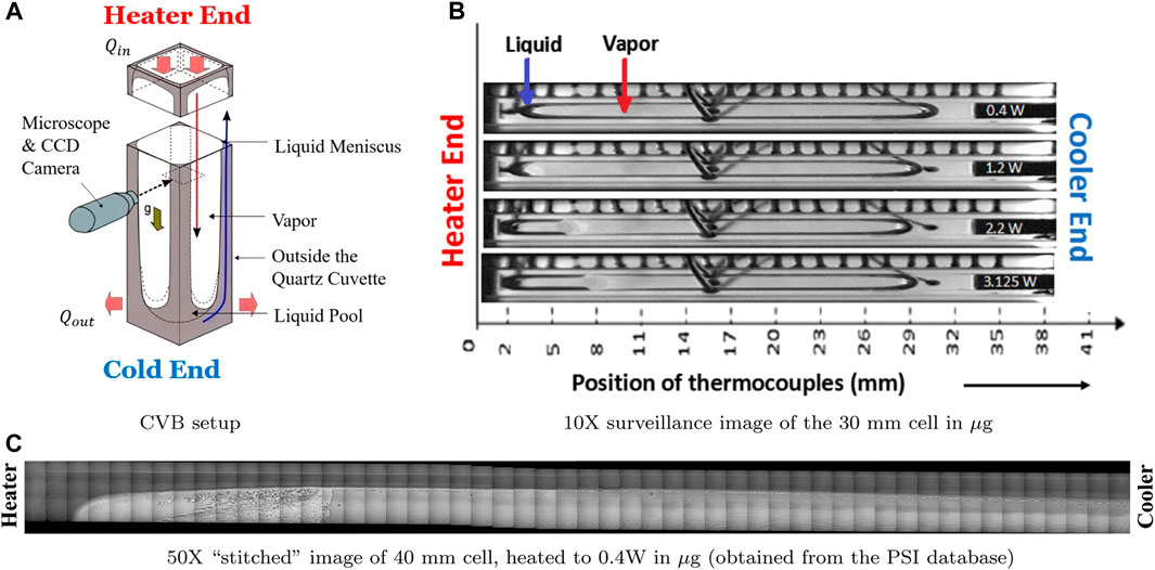
FIGURE 2. CVB experimental setup (A), sample low magnification images (B) and high magnification “stitched” images (C).

The primary objective of the CVB experiments was to investigate the fluid dynamics and heat transfer processes in an ideal wickless heat pipe in microgravity (Chatterjee et al., 2013). Heat transfer processes occurring in the microscale and their effects on the macroscale heat transfer were investigated along with the performance limits of the micro heat pipe. Quartz cuvettes, 5.5 mm × 5.5 mm on the outside and 3 mm × 3 mm on the inside were used. Cuvettes of different lengths (20 mm, 30 mm, and 40 mm) were tested. Thermocouples (±0.5 K) were embedded 0.5 mm into the wall along the length every 1.5 ± 0.1 mm. A pressure transducer (0–350 kPa, ±600 Pa) was used to monitor the bulk liquid pressure. The Light Microscopy Module (LMM) was used to image interferometric fringe patterns that indicate local interface curvature gradients. In order to observe multiple scales of the CVB experiment, two sets of images were obtained: macroscopic 10× (shown in Figure 2B) and microscopic 50× (Chatterjee et al., 2011b). Since the cuvette was optically transparent and flat, the microscope was used to capture the reflectivity between the fluid and the inside surface of the cuvette (Chatterjee et al., 2013). This produced an interference pattern near the liquid-vapor interface and can be seen in the 50× images. The individual microscopic (50×) images from the steady state operation were assembled to form a composite or “stitched” image for the reconstruction of the vapor bubble shape as shown in Figure 2C. In order to characterize the heat loss to the environment, experiments were conducted with an evacuated cuvette, and the thermal response was recorded.

At heat inputs greater than 2 W, the liquid was observed to flood the heater end of the cuvette (Kundan et al., 2015; Kundan et al., 2016). This is contrary to analogous experiments conducted on Earth in which the heater end dries out. Accumulation of liquid at the heater eventually results in the formation of a central liquid drop, as shown in Figure 2B.

1.5 Current study

The CVB experiments provide a broad dataset of interferometric images of the axisymmetric bubble which can be used to determine curvature and disjoining pressure along the curved interface of the bubble and computationally resolve the interfacial temperature and mass flux profiles using methods discussed in the following sections. Using liquid film profiles and temperature distributions from the experimental dataset available in NASA’s Physical Sciences Informatic (PSI) database (Payne, 2020), the current work aims to use a combination of image processing, thermal analysis, and a computational model to investigate a wavy fluid flow pattern observed near the heater in the experimental setup. The interface reconstruction, thermal characterization, and a multi-scale model are described herein. The bubble is assumed to be in a steady state. The high-resolution images in Figure 2C do not provide data near the condensing end. However, in microgravity, surface tension dominates, and any droplet/bubble tends to have a shape with the lowest surface area, which is generally that of a sphere, as seen in Figure 2B. Hence, a spherical cap assumption is made while reconstructing the ends of the bubble in the coming sections. Using a unique coupling between phase change models at the micro and macro (bulk) length scales, experimentally observed flow patterns are investigated, described, and explained. The objective of the current effort is to elucidate the role of thermocapillary effects on complex internal flow patterns. Here, tangential stresses on the liquid-vapor interface were included by implementing a temperature-dependent surface tension model to account for thermocapillary flow along the liquid-vapor interface. The results show that the wavy flow patterns observed in the experiments are due to thermal Marangoni flow along the interface that has the potential to grow further into instabilities and cause heater-side flooding at higher heat inputs.

2 Materials and methods

2.1 Image analysis and surface reconstruction

During the CVB experiment, monochromatic light (λ = 546 nm) is incident on the cuvette. The light reflects partially at the solid-liquid surface and partially at the curved liquid-vapor interface of the bubble. As light travels at different speeds in different media, a phase shift is created between the two reflected beams and causes interference. As the height of the curved liquid film changes, the phase shift changes proportionally, creating a fringe pattern. These fringe patterns are imaged at various locations and stitched into a composite image as shown in Figure 3. The resulting images are 2,234 × 20,789 pixels, with each pixel being a square of 0.012 mm. The 8-bit images contain pixel intensity values, G, between 0 and 255. A typical line scan along the region represented by the blue arrow in Figure 3 is shown in Figure 4A.

FIGURE 3

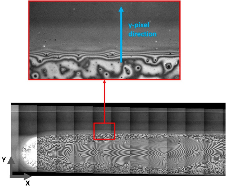
FIGURE 3. Due to a relative reflectivity and a gradually varying liquid film thickness, an interferometric fringe pattern is seen in the thin film region. Film thickness can be calculated by the spatial variance in the pixel intensities scanned in the direction shown by the blue arrow in the image. The obtained pixel intensities are plotted in Figure 4A and then normalized and converted to film thickness profiles.

FIGURE 4

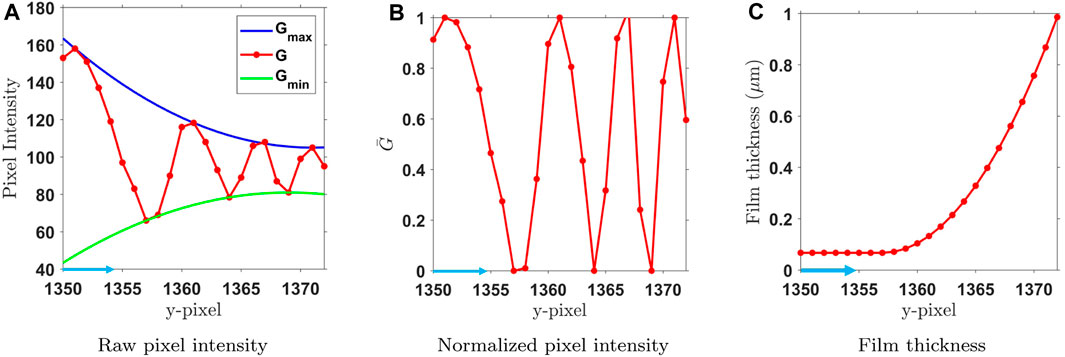
FIGURE 4. The raw pixel intensities along a line-scan (A) are normalized (B) based on the max and min enveloping curves. The normalized intensity is fitted with a theoretical sinusoidal oscillatory function to extract local film thickness data from each pixel. The blue arrow indicates the direction in which pixels are scanned for intensities, as shown in Figure 3. (C) Film thickness.

The maxima and minima of the oscillating G values are identified for each scan. G_min and G_max, shown in Figure 4A are fitted quadratic envelopes of the maxima and minima of the grayscale function, G. These envelop curves are fitted to the data with an R² value of 0.99 or higher. These envelopes are then used to normalize the global variation in the grayscale function:

$\bar{G}\left(y\right)=\frac{G\left(y\right)-G_{\min }\left(y\right)}{G_{\max }\left(y\right)-G_{\min }\left(y\right)}(5)$

The normalized $\bar{G}$ function (Figure 4B) is then used to compute the film thickness in a manner similar to Panchamgam et al. (Panchamgam et al., 2005). First r₁ and r₂ are defined as functions of the refractive indices of the liquid, solid, and vapor given by n_l and n_s and n_v respectively:

$r_1=\frac{n_l-n_v}{n_l+n_v}(6)$

$r_2=\frac{n_s-n_l}{n_s+n_l}(7)$

The relative reflectivity of the liquid film is a function of the $\bar{G}$ given by

$RL=\bar{G}\left[R{L}_{\mathit{max}}-R{L}_{\mathit{min}}\right]+R{L}_{\mathit{min}}(8)$

where,

$R{L}_{\mathit{max}}={\left(\frac{r_1+r_2}{1+r_1{r}_2}\right)}^2(9)$

$R{L}_{\mathit{min}}={\left(\frac{r_1-r_2}{1-r_1{r}_2}\right)}^2(10)$

The film reflectivity in terms of film thickness is given by,

$RL=\frac{a+bcos2\varphi }{K+bcos2\varphi }(11)$

where,

$a=r_1^2+r_2^2(12)$

$b=2r_1{r}_2(13)$

$K=1+r_1^2{r}_2^2(14)$

$\varphi =\frac{2\pi n_l\delta }{\lambda }(15)$

From equation Eq. 8, 11, film thickness $\left(\delta \right)$ can be expressed as a function of $\bar{G}$,

$\delta =\frac{\lambda }{4\pi n_1}{\cos }^{-1}\left(\frac{b+K\left(1-2\bar{G}\left(y\right)\right)}{b\left(2G\left(y\right)-1\right)-K}\right)(16)$

Hence, Eq. 16 can be used to calculate local film thickness (δ) (Figure 4C) along a single line scan in the y-direction (Figure 3). Using this technique, each pixel essentially becomes an individual film thickness sensor. However, the technique is limited to film thicknesses $<$0.25 mm. As the line scan moves toward the thicker bulk region of the liquid, this type of analysis fails as the intensity variation between the maxima and minima reduces (Figure 4A and the resolution of the fringe patterns is no longer enough to calculate film thickness satisfactorily. Panchamgam et al. (2005) reported a film thickness calculation error of ±0.1 μm in the bulk and transitional film regions and an error of 10% of the film thickness in the adsorbed film region. Therefore, the remaining film profile is reconstructed using quadratic extrapolation, assuming the bubble to be four-way symmetric at the 0 W heat setting (Figure 5A).

FIGURE 5

FIGURE 5. Symmetry is used to model a 1/8th section of the bubble. Part of the film is reconstructed by interferometric analysis. The remaining is extrapolated to the 45° symmetry line. (A) Lines of symmetry. (B) Extrapolation to symmetry line.

Figure 5B shows the film profile reconstructed for 1/8th of the geometry due to the multiple symmetry conditions. Interferometric analysis enables reconstructions of film thickness $<$0.2 mm. Quadratic extrapolation is then used to patch the rest of the surface with the condition that the slope is exactly equal to unity at the diagonal symmetry line (Figure 5B). The process is repeated at different axial slices in the x-direction, enabling a two-dimensional surface reconstruction. Due to insufficient data near the axial ends of the bubble, a spherical cap approximation is used to patch the surface profile. The overall film thickness ranges from millimeters to a nanometer. This multiscale variation of lengths makes it difficult to perform traditional CFD. Hence, the film profile must be truncated. Small cutoff thicknesses ($<\mathrm{1 }\mu$m) result in a high computational cost, while cutoff thicknesses greater than 30 μm exhibit a gradual deviation in results. A cutoff thickness of 10 μm was found to be optimum. The phase change from the truncated film below 10 μm is modeled through a separate microscale thin model, as discussed in the proceeding sections. The final reconstructed surface of the bubble is shown in (Figure 6). The macroscopic shape corresponds to that obtained by surface area minimization tools (such as surface evolver). However, there is deviation near thin film regions and/or at higher heat inputs. The microscale shape depends on a coupling between phase change dynamics, thin film evaporation, capillary flow, and surface tension that is still poorly understood. Surface area minimization alone cannot account for this, and hence, our ability to predict microscale film profiles and/or shapes of heated bubbles is limited.

FIGURE 6

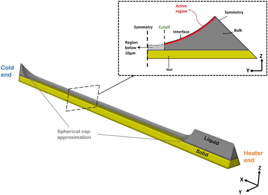
FIGURE 6. A view of the computational domain showing the yellow solid part and the gray liquid. The inset figure shows a schematic of a slice perpendicular to the bubble axis (x-direction) with the “active region” marked in red and cutoff (10 μm). The positive y-direction in the CFD domain increases towards the adsorbed film region. Phase change physics of the region below 10 μm is discussed in Section 2.4.

2.2 Thermal analysis

As part of the CVB experiment campaign, dry tests were performed where the fluid was removed and a vacuum was pulled inside the cuvette. The heater was turned on while thermocouples installed in the wall along the axial length of the cuvette measured temperatures. A one-dimensional heat balance along the outer wall of the cuvette shows that the axial conduction is balanced by heat lost into the outer environment due to radiation:

$-k_s{A}_c\frac{d^{2}T}{d{x}^2}={\sigma }_Bϵp_o\left(T^4-T_{\infty }^4\right)(17)$

where k_s is the thermal conductivity of quartz, A_c is the cross-sectional area, T is the outer wall temperature, T_∞ is the temperature of the surrounding environment, ϵ is the emissivity of quartz σ_B is the Stefan-Boltzmann constant, and p_o is the outer perimeter of the wall’s cross-section.

In the current study, ϵ and T_∞ are determined by fitting the solution for Eq. 17 to the experimentally measured temperatures. Eq. 17 is solved using the ODE45 algorithm (fourth order Runge Kutta method) in MATLAB (Figure 7). The boundary conditions are known experimental parameters: constant heat flux at the heater and constant temperature at the cooler end. A view factor of unity is assumed for radiative heat transfer. The values of ϵ and T_∞ are determined to be 0.773 and 293 K, respectively. The average ambient temperature on board the ISS has been reported to be 20°C (Plawsky and Wayner, 2012), which is in good agreement with the results of this study. These parameters are used as inputs for boundary conditions discussed in the next section.

FIGURE 7

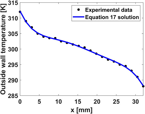
FIGURE 7. Experimental temperature measurements at the outside wall are used to obtain optimized emissivity and surrounding temperature values. Equation 17 is solved and compared to the experimental data. The emissivity and surrounding temperatures are then used as boundary condition parameters in the computational analysis (Section 2.3).

2.3 Macroscale CFD

The reconstructed liquid-solid domain is discretized to 167,944 mesh cells and implemented in Ansys Fluent. Figure 6 shows the liquid domain in gray and the solid wall in yellow. The apex tips of the hot and cold ends are located at x = 5 mm and 29.7 mm. Laminar flow is assumed in the liquid with a no-slip boundary condition on the inner solid wall. Two symmetry boundary conditions are applied as shown in Figure 6. A heat flux boundary condition of 6,611.57 W/m² at the heater end of the domain to match the condition of 0.2 W heater power setting used during the experiments. The cold end is set to a constant temperature of 288 K based on the experimental setup (Chatterjee et al., 2011a). The error from the experimental setup is anticipated to be less than 1 K. A radiative heat flux boundary condition is used at the outer wall, based on ϵ and T_∞ obtained from the thermal analysis (section 2.2). Thermophysical properties for n-pentane are obtained from the NIST website (Linstrom, 1997) and quartz density is set to 2,719 kg/m³ and thermal conductivity is set to 1.4 W/m − K.

Assuming the vapor phase is in equilibrium and the bubble is at a steady state, only the liquid domain is modeled. To account for phase change at the interface, a single-cell thick layer of mesh cells in the liquid domain, adjacent to the interfacial surface is selected as the “active region” as shown in the inset of Figure 6. The marked cells represent the region undergoing phase change-related heat and mass transfer. In the active region, User-Defined Functions (UDFs) are used to compute the local mass flux based on Wayner’s phase change model (Eq. 2) with constant vapor properties and locally queried liquid properties. Heat flux is computed by multiplying mass flux with the enthalpy of evaporation of n-pentane. These computed fluxes are included in the simulation as source or sink terms in the active region, creating mass and heat in the liquid in regions of condensation and removing mass and heat in regions of evaporation. Surface tension is modeled as a linear function of liquid temperature at the interface:

$\sigma ={\sigma }_1+\frac{d\sigma }{d{T}_i}{T}_i(18)$

where, σ₁ has a value of 0.0476 N/m and $\frac{d\sigma }{d{T}_i}$ has a value of −0.0001 N/m-K (Linstrom, 1997). The Marangoni stress function is turned on, allowing Ansys Fluent to evolve surface tension based on interfacial temperatures (Eq. 18).

A zero heat and mass flux boundary condition is initially used at the cut-off plane (10 μm). This is relaxed in subsequent iterations. Steady-state mass, momentum, and energy equations were solved using the SIMPLEC pressure-velocity coupling in Ansys Fluent. The user-defined phase change model is integrated into the CFD solution such that it determines the local interfacial mass flux and temperatures until convergence is reached. The inside wall temperatures are extracted and used to determine mass flux contributions from the cut-off thin film below 10 μm, as described in the next section.

2.4 Thin film modeling

Phase change physics in the film below 10 μm (cutoff region) is ignored in the CFD domain. However, an independent thin film model is used to solve for the net mass and heat transfer at the liquid-vapor interface in this region. The crux of the model is a 1D heat balance where heat conduction from the solid wall to the interface is balanced with the phase change heat flux at the interface. The wall temperature boundary condition that is informed by the macroscale CFD model is non-uniform and this inherently incorporates the wall conduction in both the x and y directions. We do not assume that the wall temperature at a specific x location is constant/uniform but instead is variable, as described in Figure 8. Furthermore, the temperature gradient across the film (z-direction) is much larger than along the film (in either x or y directions) due to the orders of magnitude difference in the length scales. Hence, a 1D approximation is appropriate in the microscale thin film where the heat loss due to evaporation is balanced by conduction through the liquid:

$h_{\text{fg}}{\dot{m}}^{″}=-k_l\frac{T_w-T_i}{\delta }(19)$

FIGURE 8

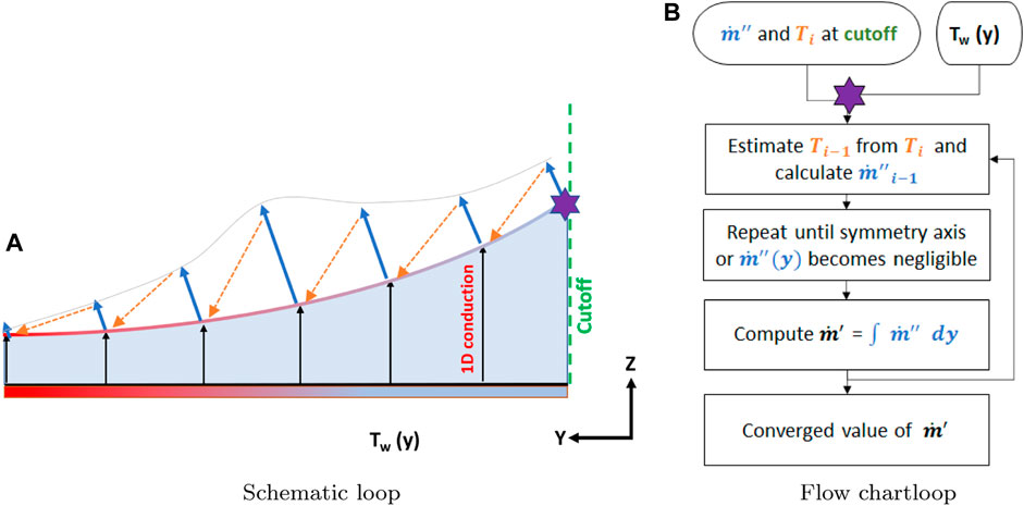
FIGURE 8. Schematic (A) and flow chart (B) representing the iterative loop in thin film analysis. The positive y-direction is towards decreasing film thickness.

Starting from the mesh node nearest to the 10 μm cutoff and stepping in a direction of reducing film thickness towards the adsorbed film, the thin film model calculates the total mass flux in the cutoff region. The process is depicted in Figure 8B. Interface temperature, T_i, and local mass flux, ${\dot{m}}^{″}$ (from 2), at the 10 μm starting point (denoted by the purple star in Figures 8A, B) along with solid wall temperature profile (T_w(y)) from the initial CFD simulation are used as inputs. Using the film thickness (δ) obtained from image processing Eq. 19 is used to calculate a new value of T_i and a local mass flux ${\dot{m}}^{″}$ for the next step. The process is repeated till either the symmetry plane (y = 1.5 mm) is reached or the local ${\dot{m}}^{″}$ becomes negligible. By coupling the thin film model with the macroscale CFD, a continuous, smooth mass flux distribution along the entire surface can be obtained. Figure 9 shows the converged mass flux distribution and the film profile for the transition film at a distance of 9 mm from the heater. The mass flux peaks at a film thickness of 46 μm. As expected, the film thickness and mass flux reduce toward the adsorbed film region.

FIGURE 9

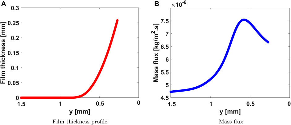
FIGURE 9. Numerical solution for the mass flux and film thickness profiles at an axial location of 9 mm from the heater. (A) Film thickness profile. (B) Mass flux.

This process described above is repeated for all axial locations along the CVB. Once a continuous mass flux profile is available, the mass flux in the cutoff regions is extracted and integrated over the corresponding film length to obtain ${\dot{m}}^{\prime }(x)$, as shown in Figure 10, such that it can be used as a boundary condition in the macroscale CFD thereby relaxing the no-mass flux at cutoff assumption.

FIGURE 10

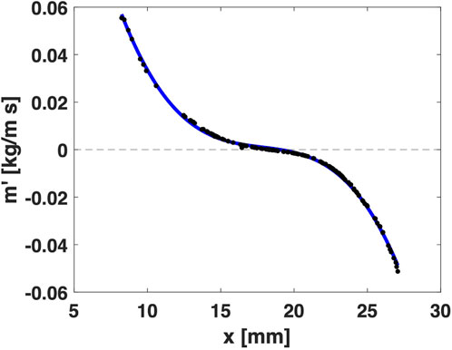
FIGURE 10. Mass flow rate per unit length profile integrated in the transverse direction.

The macroscale CFD model and the thin film model are solved iteratively. Interface temperature at the cutoff and inner solid wall temperatures from the CFD model are used as inputs to the transition film model, and the mass flux from the thin film model is fed back to the macroscale CFD model in subsequent iterations. The combined model is iterated until the inner wall temperature changes less than 0.1% between successive iterations. The coupled model is devoid of guessed/arbitrary matching conditions and relies solely on experimental inputs. In recent studies, this strategy has been successfully employed by the authors (Bellur et al., 2020; Bellur et al., 2023) to obtain a smooth multiscale mapping of phase change. This technique allows for non-uniformity in phase change, resulting in non-uniform temperature and subsequent interfacial flow, as discussed in the next section.

3 Results and discussion

3.1 Mass flux and temperature profiles

Figure 11 shows the mass flux and interface temperature distribution across the liquid-vapor interface. The 2D contour plots shown here are projections of the surface as seen vertically downward in the negative z direction as shown by the green arrow in Figure 11. In the vicinity of the heater, the mass flux is positive, indicating evaporation with a peak flux of approximately 20 mg/m²s. The mass flux gradually reduces when moving away from the heater, eventually crossing zero and reaching a minimum of about −10 mg/m²s near the cooler end.

FIGURE 11

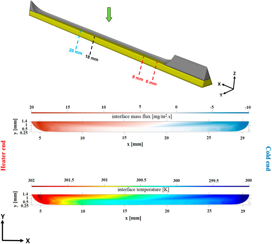
FIGURE 11. Computational results of mass flux and temperature along the interface. The results are plotted along a projection on the xz-plane viewed from above (green arrows).

Interfacial temperature shows a distribution similar to mass flux. The interfacial temperature variation is $<$3 K, with higher temperatures occurring near the heater and decreasing toward the cooler end. Non-uniformity in mass flux is also observed along the transverse direction, with a higher magnitude of both evaporation and condensation flux observed near the cutoff and is attributed to higher phase change flux from the micro-scale thin film region. Although the temperature variation is $<$3 K, this thermal non-uniformity induces interfacial Marangoni flow which is in the opposite direction to the capillary flow in the bulk. Complex flow patterns are observed due to the interaction of the interfacial and capillary mass transport. These flow patterns are visualized in the next section.

3.2 Velocity profiles

In the axial direction, evaporation and condensation result in capillary-driven mass transport in the bulk liquid from the cooler to the heater end. However, due to the phase change-driven interfacial temperature gradient, the heater end experiences lower surface tension than the cooler end. This surface tension imbalance causes opposing mass transport along the interface from the heater end toward the cooler end. The net effect of these opposing flow directions shows vortices near the interfacial region as seen in the brown framed box (C) in Figure 12. The red framed box (A) in Figure 12 shows velocity vectors pointing towards the micro-scale thin film region in the evaporation dominant region. However, in the condensation dominant region, the velocity vectors point away from the thin film region, as shown in the blue framed box (B). This signifies the presence of possible stagnation points and recirculation zones.

FIGURE 12

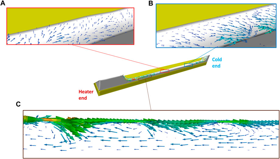
FIGURE 12. Flow pattern obtained from the CFD model. (A) velocity vectors near the heater region, (B) velocity vectors near the cooler end, and (C) recirculating wavy flow patterns in axial direction.

To better understand these flow patterns, streamlines are shown for four 2D slices perpendicular to the axis of the bubble. Two slices in the evaporation dominant region (6 and 8 mm), one in the condensing region (20 mm), and one in-between (18 mm) are shown in Figure 13. Corresponding tangential velocities, as well as mass flux and temperatures along the interface, are also shown. At the x = 6 mm slice, multiple vortices are evident. The interfacial velocities are non-monotonic. Two stagnation points (instances of zero crossing) are observed and are shown with red markers. In general, higher evaporation flux in the thin film establishes a bulk flow towards the thin film region. However, in the region between the two stagnation points 0.5–0.3 mm, the flow is negative, suggesting that the flow is reversed, i.e., away from the thin film. This is because higher temperatures in the thin film result in lower surface tension. A temperature gradient is established that results in an interfacial thermal Marangoni flow in a direction opposite to the bulk flow. However, this is short-lived since a strong evaporative flux induces a bulk flow toward the thin film that eventually overcomes the thermal Marangoni flow at a film thickness greater than approximately 0.15 mm.

FIGURE 13

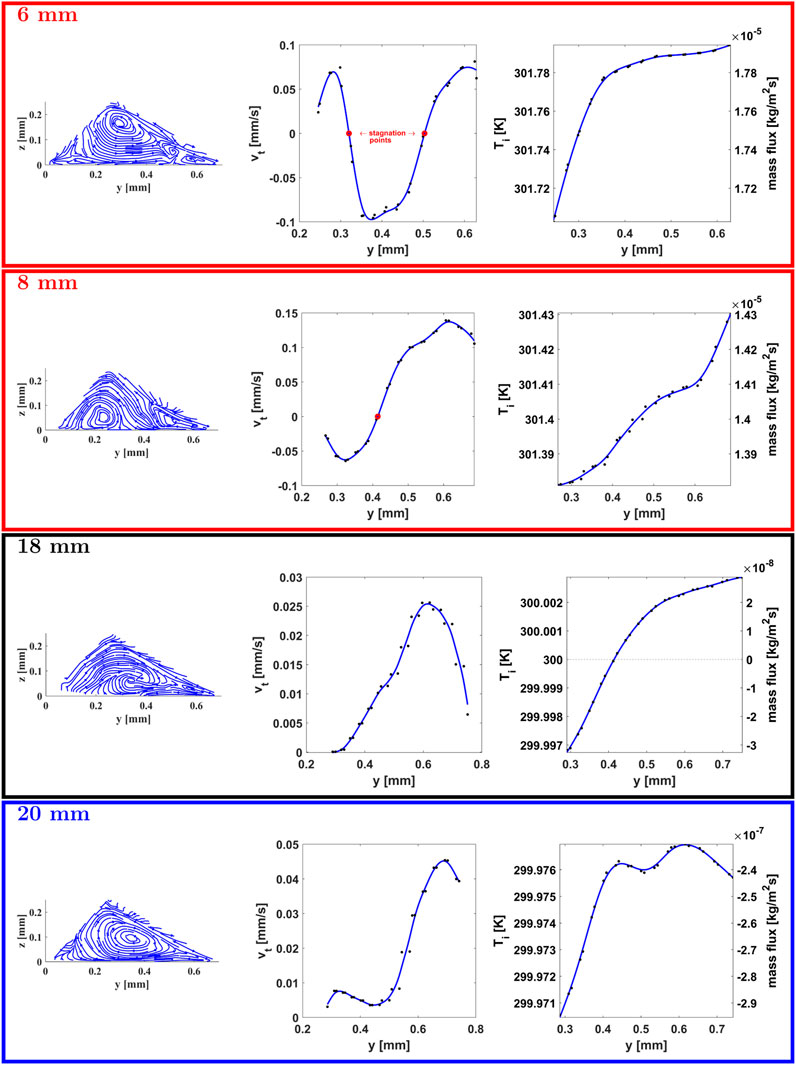
FIGURE 13. Flow patterns, velocity tangent to the interface (v_t), interface temperature (T_i), and phase change mass flux (kg/m²s) are shown as a function of the transverse coordinate (y) for slices at four axial locations (x), 6, 8, 18, and 20 mm.

At the x = 8 mm slice, only the second stagnation point is observed, and the first one disappears. The only stagnation point moves to y = 0.4 mm, i.e., moves toward the bulk region. Further moving away from the heater region (at x = 18 mm and x = 20 mm), the stagnation points vanish. However, the net evaporation becomes a net condensation mass flux as evidenced by a change in the sign of the calculated mass flux. The slice at x = 18 mm is particularly interesting since the mass flux crosses the x-axis (marked by a horizontal dotted line), and a clear evaporation/condensation zone is observed. At x = 20 mm, there are no stagnation points and is completely condensation-dominant.

Marangoni flow is dominant only near the heater end and is explained by the magnitude of the temperature variation in the transverse direction. At the heater end, x = 6 mm, the temperature variation is 0.08 K, which gradually reduces to 0.04 K at x = 8 mm and 0.004 K at x = 18 mm and 20 mm. Hence, moving toward the cooler, the temperature variation becomes smaller, and the effect of the Marangoni force reduces. The velocity contours do not vary as much, and stagnation points disappear. On the other hand, higher thermal gradients near the heater strongly influence temperature-dependent interfacial surface tension. This surface tension variation, combined with high evaporative mass flux in the thin film near the heater end, creates a complex flow pattern with multiple recirculation zones. This is likely the reason for the onset of instabilities and heater flooding observed at higher heat settings.

A combination of this orthogonal variation of flow velocities in both the axial and transverse directions results in a wave-like flow pattern along the interfacial length of the bubble, even for minimal temperature gradients. This provides further evidence of flow recirculations occurring as a result of Marangoni forces induced by a non-isothermal interface. Kundan et al. (Kundan et al., 2017) observed the formation of junction vortices at higher heater settings (3.125 W) as a result of liquid flooding into the vapor bubble near the heater side, which was an unusual phenomenon as it is expected that the heater end would dry out due to evaporation. However, in microgravity, dominant Marangoni forces affected the flow patterns near the heater, causing the liquid to recirculate back near the heater end, forming junction vortices and multiple stagnation points. Applying a heater setting boundary condition as low as 0.2 W generates recirculating flow patterns and stagnation points along the interfacial length near the heater. To correlate the above results with experimental data, the location of velocity fluctuations near the thin film region is compared with regions of non-uniform fringe patterns in the liquid film from the experimental image in the proceeding section.

3.3 Comparision with experimental images

Liquid y-velocities near the cutoff in the CFD model were qualitatively compared to the optical signatures of interferometric images for a heater setting of 0.2 W. The 0.2 W image shows fringe patterns representing a curved liquid film. The fringe patterns move towards the axis of the bubble representing liquid transport as a result of higher evaporation. However, non-uniformity is observed in the fringe pattern as shown in Figure 14. This represents irregular wave peaks/troughs (marked by C1, C2 and C3) along the curved liquid film. The transverse y-velocities are plotted along the cutoff region from the CFD model. The location of this non-uniformity in fringe patterns is in close proximity to the region of transverse velocity fluctuations at the cutoff observed in the CFD results. The y-velocity profile shows multiple inflection points along the axial direction. The y-velocities first increase from 0 to 0.22 mm/s, drop to 0.1 mm/s, and then increase to 0.15 mm/s, moving in the x direction along the cutoff. This variation in velocity agrees well with the location of C1, C2, and C3 from the experimental image with 0.2 W heater setting. It must be noted that the shape of the interface in the CFD is from the 0 W setting. Even with this shape, applying a 0.2 W heat input shows velocity fluctuations in the same region where wave peaks/trough patterns are observed in the experimental 0.2 W interferometric images from the CVB setup. This provides a qualitative correlation between obtained CFD results and experimental CVB results.

FIGURE 14

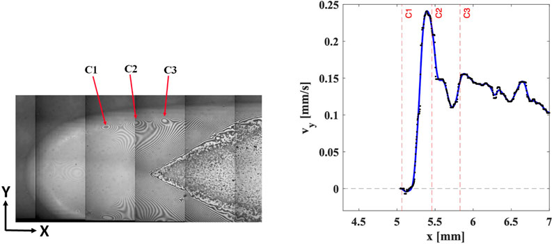
FIGURE 14. Location of wave trough/peaks along fringe patterns in the interferometric image taken at 0.2 W heater setting co-located with transverse y-velocities along the cut-off in the axial direction from the CFD results. The wedge-shaped feature at the right side of Figure 14 denotes the adsorbed film as evidenced by a lack of fringe patterns.

4 Summary

Data from the Constrained Vapor Bubble experiments conducted aboard the International Space Station in microgravity are analyzed to reconstruct a computational domain to study phase change effects in curved interfaces. A single-cell thick layer of mesh cells along the interface is separated and used to model phase change. Wayner’s equation for phase change mass flux in a curved liquid-vapor interface is used. Phase change flux in the micro-scale transition film region is solved separately from the CFD model and later integrated as a boundary condition. Boundary conditions based on the experimental setup are used to define the computational model. Temperature and mass flux distributions are calculated across the surface of the bubble. Non-uniformity is observed in the interface temperature and mass flux. This gradient induces Marangoni forces along the interface due to varying surface tension. Flow recirculations observed in the CFD model are a result of Marangoni-based interfacial motion and bulk capillary motion of the fluid. In the axial direction, the bulk liquid tends to move in a direction opposite to the interfacial motion of the liquid causing recirculating vortices and wavy flow patterns near the interface. Looking at tangential velocity plots in the transverse y-direction, multiple stagnation points are observed as a result of Marangoni forces and high evaporative flux near the heater. Reduction in thermal gradients upon moving away from the heater reduces the effect of Marangoni forces. Correlating the results with experimental data, optical signatures of interferometric images from CVB experiments also show non-uniformity in fringe patterns which are found to be in the region of velocity fluctuations near the cutoff.

The present work challenges the long-standing assumption of an isothermal interface during phase change and reveals that interfacial Marangoni flows dominate in microgravity. This leads to recirculations, stagnation points, and wavy flow patterns in the bulk liquid. Comparison with experimental data suggests that Marangoni-induced recirculation is the likely cause of meniscus instability and heater flooding observed in microgravity.

Data availability statement

The raw data supporting the conclusion of this article will be made available by the authors, without undue reservation.

Author contributions

UC: Formal Analysis, Investigation, Software, Visualization, Writing–original draft. AY: Formal Analysis, Investigation, Software, Visualization, Writing–original draft. KB: Formal Analysis, Investigation, Conceptualization, Funding acquisition, Methodology, Resources, Supervision, Writing–review and editing. JA: Conceptualization, Funding acquisition, Methodology, Project administration, Resources, Supervision, Writing–review and editing.

Funding

The author(s) declare financial support was received for the research, authorship, and/or publication of this article. This work was supported by a Physical Sciences Informatics Grant from NASA’s Physical Sciences Research Program (Grant #80NSSC19K0160). This work also received support from the University of Cincinnati through a Graduate Incentive Award for UC and AY.

Conflict of interest

The authors declare that the research was conducted in the absence of any commercial or financial relationships that could be construed as a potential conflict of interest.

Publisher’s note

All claims expressed in this article are solely those of the authors and do not necessarily represent those of their affiliated organizations, or those of the publisher, the editors and the reviewers. Any product that may be evaluated in this article, or claim that may be made by its manufacturer, is not guaranteed or endorsed by the publisher.

Supplementary material

The Supplementary Material for this article can be found online at: https://www.frontiersin.org/articles/10.3389/frspt.2023.1263496/full#supplementary-material

References

Badam, V., Kumar, V., Durst, F., and Danov, K. (2007). Experi mental and theoretical investigations on interfacial temperature jumps during evaporation. Exp. Therm. Fluid Sci. 32 (1), 276–292. doi:10.1016/j.expthermflusci.2007.04.006

CrossRef Full Text | Google Scholar

Ball, G. (2012). Numerical analysis of the heat transfer characteristics within an evaporating meniscus, Master of Applied Science. Ottawa, Ontario: Carleton University. doi:10.22215/etd/2012-07041

CrossRef Full Text | Google Scholar

Bellur, K., Médici, E. F., Choi, C. K., Hermanson, J. C., and Allen, J. S. (2020). Multiscale approach to model steady meniscus evaporation in a wetting fluid. Phys. Rev. Fluids 5 (2), 024001. doi:10.1103/PhysRevFluids.5.024001

CrossRef Full Text | Google Scholar

Bellur, K., Médici, E. F., Hermanson, J. C., Choi, C. K., and Allen, J. S. (2023). Modeli ng liquid–vapor phase change experiments: cryogenic hydrogen and methane. Colloids Surfaces A Physicochem. Eng. Aspects 675, 131932. doi:10.1016/j.colsurfa.2023.131932

CrossRef Full Text | Google Scholar

Bhunia, A., and Kamotani, Y. (2001). Flow around a bubble on a heated wall in a cross-flowing liquid under microgravity condition. Int. J. Heat Mass Transf. 44 (20), 3895–3905. doi:10.1016/S0017-9310(01)00032-1

CrossRef Full Text | Google Scholar

Borsi, I., Fusi, L., and Alessandro Speranza, F. R. (2011). Isothe rmal two-phase flow of a vapor–liquid system with non-negligible inertial effects. Int. J. Eng. Sci. 49 (9), 915–933. doi:10.1016/j.ijengsci.2011.05.003

CrossRef Full Text | Google Scholar

Chatterjee, A. (2010). The constrained vapor bubble heat pipe- on Earth and in space. PhD Thesis. Rensselaer Polytechnic Institute.

Google Scholar

Chatterjee, A., Plawsky, J., Wayner, P., Chao, D., Sicker, R., Lorik, T., et al. (2011a). “The constrained vapor bubble (CVB) experiment in the microgravity environment of the international Space station,” in 49th AIAA aerospace Sciences meeting including the new horizons forum and aerospace exposition (Orlando, Florida: American Institute of Aeronautics and Astronautics). doi:10.2514/6.2011-1197

CrossRef Full Text | Google Scholar

Chatterjee, A., Plawsky, J. L., Wayner, P. C., Chao, D. F., Sicker, R. J., Lorik, T., et al. (2010). Constrained vapor bubble experiment for international Space station: earth’s gravity results. J. Thermophys. Heat Transf. 24 (2), 400–410. doi:10.2514/1.47522

CrossRef Full Text | Google Scholar

Chatterjee, A., Plawsky, J. L., Wayner, P. C., Chao, D. F., Sicker, R. J., Lorik, T., et al. (2013). Constrained vapor bubble heat pipe experiment aboard the international Space station. J. Thermophys. Heat Transf. 27 (2), 309–319. doi:10.2514/1.T3792

CrossRef Full Text | Google Scholar

Chatterjee, A., Wayner, P. C., Plawsky, J. L., Chao, D. F., Sicker, R. J., Lorik, T., et al. (2011b). The constrained vapor bubble fin heat pipe in microgravity. Ind. Eng. Chem. Res. 10. doi:10.1021/ie102072m

CrossRef Full Text | Google Scholar

Clements, J. A., Hustead, R. F., Johnson, R. P., and Gribetz, I. (1961). Pulmonary surface tension and alveolar stability. J. Appl. Physiology 16 (3), 444–450. doi:10.1152/jappl.1961.16.3.444

PubMed Abstract | CrossRef Full Text | Google Scholar

DasGupta, S., Kim, I. Y., and Wayner, P. C. (1994). Use of the kelvin-clapeyron equation to model an evaporating curved microfilm. J. Heat Transf. 116 (4), 1007–1015. doi:10.1115/1.2911436

CrossRef Full Text | Google Scholar

DasGupta, S., Schonberg, J. A., and Wayner, P. C. (1993). Investigation of an evaporating extended meniscus based on the augmented young–laplace equation. J. Heat Transf. 115 (1), 201–208. doi:10.1115/1.2910649

CrossRef Full Text | Google Scholar

Derjaguin, B., Nerpin, S., and Churaev, S. (1965). Effect of film transfer upon evaporation of liquids from capillaries. Bull. RILEM 29, 93–98.

Google Scholar

Fang, G., and Ward, C. A. (1999). Temperature measured close to the interface of an evaporating liquid. Phys. Rev. E 59 (1), 417–428. doi:10.1103/PhysRevE.59.417

CrossRef Full Text | Google Scholar

Fritz, D. L. (2012). Implementation of a phenomenological evaporation model into a porous network simulation for water management in low temperature fuel cells, Doctor of Philosophy in Mechanical Engineering–Engineering Mechanics. Houghton, Michigan: Michigan Technological University. doi:10.37099/mtu.dc.etds/360

CrossRef Full Text | Google Scholar

Gouin, H., and Slemrod, M. (1995). Stability of spherical isothermal liquid-vapor interfaces. Meccanica 30 (3), 305–319. doi:10.1007/BF00987223

CrossRef Full Text | Google Scholar

Hähnel, M., Delitzsch, V., and Eckelmann, H. (1989). The motion of droplets in a vertical temperature gradient. Phys. Fluids A Fluid Dyn. 1 (9), 1460–1466. doi:10.1063/1.857323

CrossRef Full Text | Google Scholar

Hertz, H. (1882). Ueber die Verdunstung der Flüssigkeiten, insbesondere des Quecksilbers, im luftleeren Raume. Ann. Phys. 253 (10), 177–193. doi:10.1002/andp.18822531002

CrossRef Full Text | Google Scholar

Holm, F. W., and Goplen, S. P. (1979). Heat transfer in the meniscus thin-film transition region. J. Heat Transf. 101 (3), 543–547. doi:10.1115/1.3451025

CrossRef Full Text | Google Scholar

Knudsen, M. (1915). Die maximale Verdampfungsgeschwindigkeit des Quecksilbers. Ann. Phys. 352 (13), 697–708. doi:10.1002/andp.19153521306

CrossRef Full Text | Google Scholar

Kundan, A., Nguyen, T. T., Plawsky, J. L., Wayner, P. C., Chao, D. F., and Sicker, R. J. (2016). Arrest ing the phenomenon of heater flooding in a wickless heat pipe in microgravity. Int. J. Multiph. Flow 82, 65–73. doi:10.1016/j.ijmultiphaseflow.2016.02.001

CrossRef Full Text | Google Scholar

Kundan, A., Nguyen, T. T., Plawsky, J. L., Wayner, P. C., Chao, D. F., and Sicker, R. J. (2017). Condensation on highly superheated surfaces: unstable thin films in a wickless heat pipe. Phys. Rev. Lett. 118 (9), 094501. doi:10.1103/PhysRevLett.118.094501

PubMed Abstract | CrossRef Full Text | Google Scholar

Kundan, A., Plawsky, J. L., and Wayner, P. C. (2015). Effect of capillary and Marangoni forces on transport phenomena in microgravity. Langmuir 31 (19), 5377–5386. doi:10.1021/acs.langmuir.5b00428

PubMed Abstract | CrossRef Full Text | Google Scholar

Lakew, E., Sarchami, A., Giustini, G., Kim, H., and Bellur, K. (2023). Thin film evaporation modeling of the liquid microlayer region in a dewetting water bubble. Fluids 8 (4), 126. doi:10.3390/fluids8040126

CrossRef Full Text | Google Scholar

Linstrom, P. (1997). NIST chemistry WebBook. NIST Stand. Ref. Database 69. doi:10.18434/T4D303

CrossRef Full Text | Google Scholar

Marangoni, C. (1871). Ueber die Ausbreitung der Tropfen einer Flüssigkeit auf der Oberfläche einer anderen. Ann. Phys. Chem. 219 (7), 337–354. doi:10.1002/andp.18712190702

CrossRef Full Text | Google Scholar

Nallani, M., and Subramanian, R. (1993). Migrat ion of methanol drops in a vertical temperature gradient in a silicone oil. J. Colloid Interface Sci. 157 (1), 24–31. doi:10.1006/jcis.1993.1153

CrossRef Full Text | Google Scholar

Panchamgam, S. S., Gokhale, S. J., Plawsky, J. L., DasGupta, S., and Wayner, P. C. (2005). Experiment al Determination of the effect of disjoining pressure on shear in the contact line region of a moving evaporating thin film. J. Heat Transf. 127 (3), 231–243. doi:10.1115/1.1857947

CrossRef Full Text | Google Scholar

Payne, C. (2020). Physical Sciences Informatics (PSI).

Google Scholar

Pecenko, A., Kuerten, J., and Van Der Geld, C. (2010). A diffuse-interface approach to two-phase isothermal flow of a Van der Waals fluid near the critical point. Int. J. Multiph. Flow 36 (7), 558–569. doi:10.1016/j.ijmultiphaseflow.2010.03.005

CrossRef Full Text | Google Scholar

Plawsky, J. L., Ojha, M., Chatterjee, A., and Wayner, P. C. (2008). Review of the effects of surface topography, surface chemistry, and fluid physics on evaporation at the contact line. Chem. Eng. Commun. 196 (5), 658–696. doi:10.1080/00986440802569679

CrossRef Full Text | Google Scholar

Plawsky, J. L., and Wayner, P. C. (2012). Explos ive nucleation in microgravity: the Constrained Vapor Bubble experiment. Int. J. Heat Mass Transf. 55 (23-24), 6473–6484. doi:10.1016/j.ijheatmasstransfer.2012.06.047

CrossRef Full Text | Google Scholar

Potash, M., and Wayner, P. (1972). Evapora tion from a two-dimensional extended meniscus. Int. J. Heat Mass Transf. 15 (10), 1851–1863. doi:10.1016/0017-9310(72)90058-0

CrossRef Full Text | Google Scholar

Ruckenstein, E., and Berbente, C. (1964). The occurrence of interfacial turbulence in the case of diffusion accompanied by chemical reaction. Chem. Eng. Sci. 19 (5), 329–347. doi:10.1016/0009-2509(64)80002-6

CrossRef Full Text | Google Scholar

Sáenz, P. J., Valluri, P., Sefiane, K., Karapetsas, G., and Matar, O. K. (2014). On phase change in Marangoni-driven flows and its effects on the hydrothermal-wave instabilities. Phys. Fluids 26 (2), 024114. doi:10.1063/1.4866770

CrossRef Full Text | Google Scholar

Sawistowski, H. (1973). Surface-te nsion-induced interfacial convection and its effect on rates of mass transfer. Chem. Ing. Tech. - Cit. 45 (18), 1093–1098. doi:10.1002/cite.330451802

CrossRef Full Text | Google Scholar

Schrage, R. (1953). A theoretical study of interphase mass transfer. Ph.D. thesis. Columbia University Press.

Google Scholar

Scriven, L. E., and Sternling, C. V. (1960). The Marangoni effects. Nature 187 (4733), 186–188. doi:10.1038/187186a0

CrossRef Full Text | Google Scholar

Sultan, E., Boudaoud, A., and Amar, M. B. (2005). Evaporat ion of a thin film: diffusion of the vapour and Marangoni instabilities. J. Fluid Mech. 543 (-1), 183. doi:10.1017/S0022112005006348

CrossRef Full Text | Google Scholar

Thomson, J. (1855). XLII. On certain curious motions observable at the surfaces of wine and other alcoholic liquors. Lond. Edinb. Dublin Philosophical Mag. J. Sci. 10 (67), 330–333. doi:10.1080/14786445508641982

CrossRef Full Text | Google Scholar

Ward, C. A., and Stanga, D. (2001). Interfacial conditions during evaporation or condensation of water. Phys. Rev. E 64 (5), 051509. doi:10.1103/PhysRevE.64.051509

PubMed Abstract | CrossRef Full Text | Google Scholar

Wayner, P., Kao, Y., and LaCroix, L. (1976). The interline heat-transfer coefficient of an evaporating wetting film. Int. J. Heat Mass Transf. 19 (5), 487–492. doi:10.1016/0017-9310(76)90161-7

CrossRef Full Text | Google Scholar

Wayner, P. C. (1991). The effect of interfacial mass transport on flow in thin liquid films. Colloids Surfaces 52, 71–84. doi:10.1016/0166-6622(91)80006-A

CrossRef Full Text | Google Scholar

Wee, S.-K., Kihm, K. D., Pratt, D. M., and Allen, J. S. (2006). Microscale heat and mass transport of evaporating thin film of binary mixture. J. Thermophys. Heat Transf. 20 (2), 320–326. doi:10.2514/1.15784

CrossRef Full Text | Google Scholar

Zhao, Z., Yan, N., Li, J., Li, Z. D., Hu, W. R., and Ohta, H. (2008). Pool boiling heat transfer in microgravity. Jpn. Soc. Microgravity Appl. 25 (3). doi:10.15011/jasma.25.3.257

CrossRef Full Text | Google Scholar

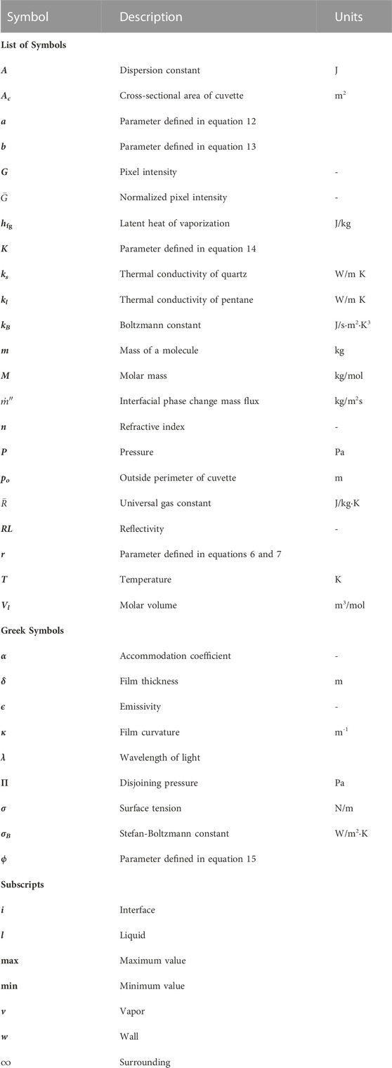
Nomenclature