 Waldemar Martens
 Lorenzo Bucci
95% of researchers rate our articles as excellent or good
Learn more about the work of our research integrity team to safeguard the quality of each article we publish.
Find out more
METHODS article
Front. Space Technol. , 30 September 2022
Sec. Space Propulsion
Volume 3 - 2022 | https://doi.org/10.3389/frspt.2022.920456
This article is part of the Research Topic Astrodynamics, Guidance, Navigation and Control (GNC) in Chaotic Multi-Body Environments View all 5 articles
Tisserand graphs are a widespread tool for interplanetary trajectory and Moon tour design. They are based on the Jacobi constant being an integral of motion in the Circular Restricted Three Body Problem (CR3BP); as such, the classical Tisserand graph does not include the perturbation of bodies other than the flyby bodies. Low-energy transfers in the Earth-Moon system make use of the combined Earth, Moon, and Sun gravities, exploiting the third body perturbations to reach the Moon with a reduced transfer Δv. The paper, therefore, proposes a novel double Tisserand graph, where the level lines of both the Earth-Moon and the Sun-Earth CR3BPs are superimposed, portraying the complex 4-body dynamics into a single plot. Paths along such level lines correspond to trajectories utilizing the dynamical effect of the Moon or the Sun or a combination of both. We show how such a graph can be efficiently used for preliminary design of Weak Stability Boundary transfers, lunar resonance transfers, lunar flybys, weak lunar captures or any combination of them.
The current plans by NASA and its partners to build a manned station around the Moon, has sparked new interest in designing transfers between the different regions in the cislunar space Whitley and Martinez (2016). Of particular interest are so-called low-energy transfers Belbruno (2018); Schoenmaekers et al. (2001); Parrish et al. (2020), that exploit the three body dynamics of either the Earth-Moon or the Sun-Earth system to reduce the transfer Δv. These transfers pass through the region where the gravitational influence of both bodies (either the Earth and Moon or the Sun and Earth) is significant and therefore their long-term evolution is chaotic. The initial guess generation for such transfers is a challenge as Keplerian dynamics cannot be used. This paper proposes a simple, graphical method based on the Tisserand-Poincaré graph that, unlike the original graph, allows finding low-energy transfers involving the effect of both the Sun and the Moon. As in the classical Tisserand graph, the phasing between the bodies and the spacecraft is neglected. This method also allows intuitively combining different techniques such as Weak Stability Boundary (WSB) transfers, lunar flybys, lunar resonances and weak lunar captures.
The Tisserand-Poincaré graph was first proposed in Strange and Longuski (2002) for the design of multi-flyby missions in the Solar System. The basic idea is to plot level lines of constant infinite velocity with respect to the flyby planet (or equivalently: level lines of the Jacobi integral of the respective Sun-planet CR3BP) in a graph where the two axes represent the perihelion radius and the orbital period (or equivalently: the aphelion radius). A point in such a graph represents a heliocentric, planar, Keplerian orbit. A planetary flyby can be represented by a displacement along a level line. The minimum flyby altitude determines the maximum distance that can be traveled along a level line. By superimposing the level lines of all planets in the Solar System in the same graph, suitable planet sequences and intermediate orbit parameters for interplanetary transfers can easily be identified. This method was afterwards used for multi-body transfers by many authors, e.g., Campagnola and Russell (2010); de la Torre Sangrà et al. (2021); Bellome et al. (2020). More recently, an extended version of the Tisserand graph has been proposed to be used in combination with small manoeuvres for low-energy transfers Campagnola et al. (2014) (so-called Tisserand-leveraging transfers) and the design of low-energy endgames for Moon tours. Reference Yárnoz et al. (2016); Ross and Scheeres (2007) discusses the use of such a Tisserand graph in the Earth-Moon system leveraging the Sun gravity.
In this paper we combine and unify all those techniques in a single plot. In particular, the approach is to plot two sets of level lines in a graph where the axes are the perigee and apogee radii of the spacecraft orbit. The first set of level lines are derived from the Jacobi integral of the Earth-Moon system. They represent lines of constant infinite velocity with respect to the Moon for orbits that cross the Moon orbit. These are the level lines that are traditionally used in Tisserand graphs. The second set of level lines are derived from the Jacobi integral of the Sun-Earth system and are plotted in the same graph. They represent the effect of the Sun that is used in the WSB transfer.
The document is structured as follows: After an introduction of the main concept in Section 2, Sections 3.1, 3.2, 3.3 and 3.4 discuss how to use the double Tisserand graph to design WSB transfers, lunar resonance transfers, flybys and weak lunar capture trajectories, respectively. Following a short word on maneuvers in Section 3.5, Section 4 presents examples of how to use a combination of these techniques to design low-energy transfers to a Near-Rectilinear Halo Orbit (NRHO). The paper closes with a discussion in Section 5. Detailed derivations are available in the Supplementary Appendix (Sections 6 and 7).
All equations in this paper use adimensional units. Plots are dimensionalized to the Sun-Earth-Moon system.
Tisserand graphs are based on the conservation of the Jacobi integral in the CR3BP. In adimensional units of the synodic reference frame, the Jacobi integral can be computed as follows:
Here, μ is the (adimensional) gravitational constant of the lighter (secondary) body, and (1 − μ) the gravitational constant of the heavier (primary) body. The latter can be either the Sun or the Earth for the purpose of this paper. The mean motion of the system, n, is unity in the adimensional system, but is kept in the equations for traceability. x, y, z,
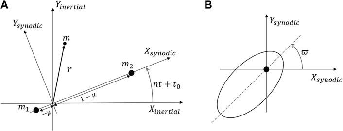
FIGURE 1. The synodic reference frame in the CR3BP (A), with definition of longitude of pericenter, ϖ (B).
Figure 1B defines the longitude of pericenter, ϖ, computed in the synodic frame, which is used throughout the paper to characterize transfers. Finally, r1 and r2 are the distances of the spacecraft from body 1 and 2, respectively. They can be computed as follows:
During parts of the spacecraft trajectory where the secondary body is the main source of gravitational attraction, Eq. 1 can be expressed in terms of osculating, Keplerian elements around the secondary body. This will be convenient for a representation of Jacobi integral level lines of the Sun-Earth system in a Tisserand graph where the axes are the perigee and apogee radii. The derivation is detailed in the Supplementary Appendix SA and results in the following expression:
No approximation has been done at this point. However, it is useful to approximate r1 and r2 by fixed values in Eq. 3 to make CJ independent of the position of the spacecraft on its orbit. This will be done later for the creation of Tisserand graphs. as, es and is are the semi-major axis, eccentricity and inclination in an inertial reference frame with the secondary at the center and the fundamental plane coinciding with the orbital plane of the two bodies.
In the other limiting case, where the spacecraft is solely under the gravitational influence of the primary body, Eq. 1 can also be expressed in terms of osculating, Keplerian elements around the primary body. With some approximations, that leads to an expression which is identical to the Tisserand parameter Roy (1978) up to a constant. The derivation of Eq. 4 and the justification of the assumed approximations can be found in the Supplementary Appendix SB:
Note, that here ap, ep and ip are the semi-major axis, eccentricity and inclination in an inertial reference frame with the primary at the center. The second line in Eq. 4 gives an alternative expression where the Jacobi integral is parameterized in terms of the infinite velocity with respect to the secondary body,
In order to analyze both Sun and Moon third body effects, we define two CR3BPs, one in the Sun-Earth system and another one in the Earth-Moon system. Eqs 3, 4 are used to express the Jacobi integrals as a function of the spacecraft Keplerian elements with the Earth at the center in both cases. In order to make Eq. 3 independent of the position of the spacecraft, the approximations r1 = 1 and r2 = 0 have been used which are valid in the close vicinity of the Earth. Moreover, only planar motion is considered. The resulting (dimensionalized) basic double Tisserand graph using the perigee and apogee radii as the independent variables is shown in Figure 2. The perigee and apogee radii, rp and ra are computed from the semi-major axis, a and eccentricity, e, as follows:
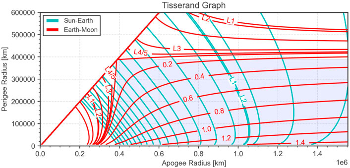
FIGURE 2. Basic double Tisserand graph showing level lines of the Jacobi integral in both the Sun-Earth and the Earth-Moon systems. In both cases, the lines corresponding to the Jacobi integral value of the libration points are indicated. For orbits crossing the Moon orbit, the numbers indicate the flyby infinite velocity in km/s.
The shaded area indicates spacecraft orbits that cross the Moon orbit and therefore allow for a lunar flyby. The red level lines in that region correspond to constant flyby v∞. They are spaced by 0.2 km/s. The red level lines extend beyond the shaded region into the low-energy regime that can be used for lunar resonance transfers (cf. Section 3.2) and weak captures at the Moon (cf. Section 3.4). The level lines that correspond to the Jacobi integral values of the Earth-Moon libration points are also indicated.
The cyan level lines, indicate the loci of constant Jacobi integral in the Sun-Earth system. They show the low-energy regime that can be used for WSB transfers leveraging the Sun gravity (cf. Section 3.1). In the following sections, the basic double Tisserand graph will be analyzed in some detail in order to generate initial guesses for low-energy transfers.
WSB transfers have been proposed in Belbruno (1987) and used by the Hiten mission in 1991 Belbruno and Miller (1993); Belbruno (2018) and more recently in the GRAIL mission Hoffman (2009). Starting with a low perigee and an apogee close to the Earth sphere of influence, the Sun gravity gradient is exploited to raise the perigee to the lunar altitude1. In this way, the total Δv can be reduced compared to standard Hohmann transfers to the Moon. Figure 3A shows two such transfers in the Earth-centered synodic Sun-Earth frame. The apogee has to point to a quadrant where the Sun gravity gradient acts along the spacecraft velocity. An apogee in one of the other two quadrants would reduce the perigee radius and can be used for transfers from the Moon back to Earth. For a fixed initial apogee radius, the longitude of perigee (defined in the synodic Sun-Earth frame) determines the final perigee radius and needs to be tuned such as to accomplish the mission needs. This is illustrated by the parametric plots in Figure 3B. The quadrant pointing away from the Sun (longitude of perigee close to 0°) is always a bit more efficient than the other in terms of perigee raising. The highest increase in perigee radius is indicated by a cross in the plot. A lower increase can always be achieved by tuning the longitude of perigee away from the extreme value.
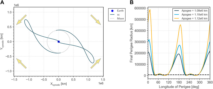
FIGURE 3. Two WSB transfers in the Sun-Earth CR3BP shown in the Earth-centered synodic Sun-Earth frame (A). The yellow arrows indicate the general direction of the Sun gravity gradient. Final perigee radius (B) for an initial perigee altitude of 300 km (dashed line) and three different initial apogee altitudes. In terms of perigee raising, the most efficient longitude of perigee is always close to 0° and 180°.
The Tisserand graph allows displaying the relationship between all relevant parameters in a very concise way as shown in Figure 4. Transfers with the longitude of perigee value maximizing the Sun effect (the maximum in Figure 3B) are represented by moving between two crosses in the Tisserand graph. One step corresponds to one orbit revolution around the Earth. Steps that are smaller than indicated by the crosses can easily be achieved by deviating from the extreme longitude of perigee value. At an initial apogee radius of around 500, 000 km the Sun effect is weak and therefore the distance between the crosses is very small. To increase the perigee to the lunar altitude would require many revolutions around the Earth, i.e. many steps in the Tisserand graph. But towards higher initial apogee radii, the distance between the crosses increases, allowing to reach perigee radii at lunar altitude or above in a single step. Note that the interesting region is where the spacecraft Jacobi integral is close to the value of the Sun-Earth L1 and L2 libration points.
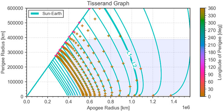
FIGURE 4. Tisserand graph showing level lines of the Jacobi integral in the Sun-Earth system. The crosses indicate the maximum possible travel distance during one revolution around the Earth. The colors of the crosses indicate the longitude of perigee at the start of the transfer which is always close to 0°. That’s why they are all the same color.
The color bar indicates the initial longitude of perigee used in the transfer (defined in the synodic Sun-Earth frame). It is always close to 0°, consistent with Figure 3B. As the perigee radius increases in the Tisserand graph, one can observe a deviation between the level lines and the crosses. This is because of the approximation made to Eq. 3 of setting r1 = 1 and r2 = 0 when computing the level lines, which is only valid close to the Earth. Nevertheless, the level lines approximate the general behavior of WSB transfers in the Tisserand graph very well.
When launching with an apogee altitude below the lunar altitude, the lunar perturbation can be used to increase the perigee and thus reduce the lunar orbit insertion Δv Schoenmaekers et al. (2001). By tuning the spacecraft orbital period at each revolution to be in resonance with the Moon, a close-to-ballistic sequence of close Moon encounters can be constructed. The effect of the lunar gravity is illustrated by the trajectories in Figure 5. Both shown trajectories have an initial perigee altitude of 10,000 km. Their apogee radii are 330,000 km (light blue) and 360,000 km (yellow), respectively. However, only the latter has an optimal phasing with the Moon, i.e., encounters the Moon in a trailing configuration. This results in the strong increase of both, the perigee and apogee radii. In the other trajectory, the perigee radius remains almost unchanged. For a fixed apogee radius, the parameter to be tuned is again the longitude of perigee, but defined in the synodic Earth-Moon frame.
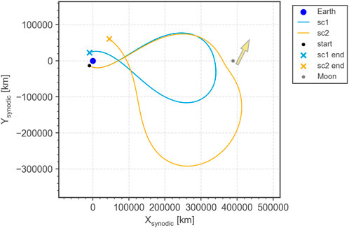
FIGURE 5. Two lunar resonance transfers in the Earth-Moon CR3BP shown in the Earth-centered synodic frame. Only the yellow trajectory has an optimal longitude of perigee which results in a strong increase of the perigee radius. The yellow arrow indicates the general direction of the lunar gravity pull.
Figure 6 shows how the final perigee and apogee radius after one revolution changes as a function of the longitude of perigee. The crosses indicate points that lead to the strongest increase of perigee radius for a given apogee radius. Smaller increases are always achievable by tuning the longitude of perigee away from the extreme value. A reduction of the perigee is also possible by choosing the longitude of perigee around 250°, i.e. encountering the Moon in a heading configuration.
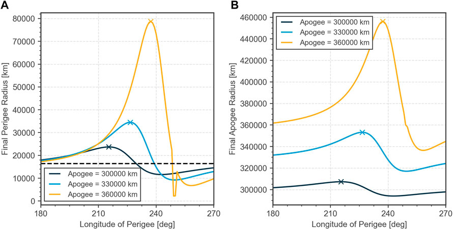
FIGURE 6. Final perigee radius (A) and apogee radius (B) for an initial perigee altitude of 10,000 km (dashed line) and three different initial apogee radii. In terms of perigee raising, the most efficient longitude of perigee is between 210° and 240°.
The maximum achievable steps in perigee radius can again be plotted in the Tisserand graph as shown in Figure 7. It is clear that the higher the initial apogee radius, the fewer steps are required to circularize the orbit. Above a certain initial apogee radius, the Moon effect raises the apogee above the lunar altitude. The plot also shows that a minimum perigee altitude is required to achieve a significant effect from the Moon perturbation. The higher the initial perigee radius, the stronger the effect becomes. The optimal longitude of perigee (measured at perigee) is always in the range 210°–240° as indicated by the color bar and consistent with Figure 6. Again, a deviation of the crosses from the level lines is observable, the higher the perigee radius becomes. This is due to the approximations done for the derivations of Eq. 4.
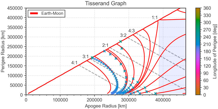
FIGURE 7. Tisserand graph showing level lines of the Jacobi integral in the Earth-Moon system and lunar resonance transfers. The crosses indicate the maximum possible travel distance during one revolution around the Earth for the longitude of perigee as indicated by the color bar. Resonance ratios with the lunar orbit are indicated by dashed lines.
Moreover, Figure 7 indicates loci in the ra − rp plane that correspond to integer period ratios with the Moon (dashed lines): for instance, 3 : 1 indicates orbits where the spacecraft performs three complete revolutions around the Earth in the same time as the Moon performs one revolution. Strictly speaking, these are only valid for purely Keplerian orbits, but can serve as a useful indication even here, where the lunar gravity is important. During the revolutions where there is no Moon encounter, the spacecraft will move on a close to Keplerian orbit. In order to design a lunar resonance sequence, it is desirable to chose the steps in the Tisserand graph such that they land on one of the resonance lines. Preferably, those are chosen where the second number is lowest, because those take the least amount of time.
The traditional way of using Tisserand graphs is for multi-flyby missions [cf. Strange and Longuski (2002); Miller and Weeks (2002)]. In the Earth-Moon system, flybys can, of course also be employed to save Δv. Due to the high relative velocity with respect to the Moon at encounter, a full three-body treatment is not required and a patched conics approach Battin (1987) yields sufficiently accurate results for the sake of initial guess generation Topputo (2013). The flyby is modeled as an instantaneous rotation of the infinite velocity vector. The rotation angle, δ depends on the flyby altitude, h, as follows:
where rMoon is the radius of the Moon, v∞ the flyby infinite velocity and μMoon the gravitational constant of the Moon. The flyby altitude takes a similar role as the longitude of perigee in Sections 3.1, 3.2 in defining the strength of the third body effect. It is also convenient to define the so-called pump angle Strange et al. (2007), which is the angle between the Moon velocity and the spacecraft infinite velocity vector at encounter. Depending on whether the flyby is performed at the left or the right side of the Moon as seen from the spacecraft, the pump angle can either be increased or decreased by the same amount. These are called the “pump-up” and “pump-down” solutions in this paper. Examples of both cases are shown in Figure 9. The final orbital parameters after a lunar flyby for both options are illustrated in Figure 8 as a function of the flyby altitude. For the shown case, the pump-down solution can even lead to an escape from the Earth-Moon system if the flyby altitude is chosen low enough.
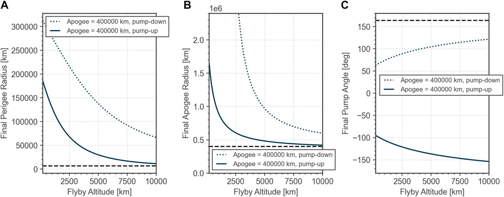
FIGURE 8. Final perigee radius (A) and apogee radius (B) and pump angle (C) after a lunar flyby for an initial perigee altitude of 300 km and an initial apogee radius of 400,000 km (dashed lines). Two solutions are possible (pump-down and pump-up depending on the flyby orientation).
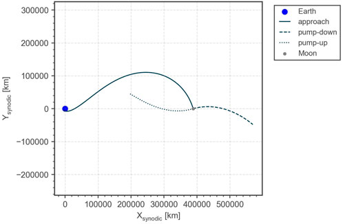
FIGURE 9. Pump-down and pump-up trajectories after a lunar flyby of 1,000 km altitude in the synodic Earth-Moon frame. This illustrates the strong effect of the lunar gravity.
The maximum travel distances along the infinite velocity level lines in the Tisserand graph are shown in Figure 10 for a minimum flyby altitude of 200 km. In the shown region, any point on the level line can be reached in a single step. The strong effect of a lunar flyby is due to the relatively high ratio of gravitational constants between the Moon and the Earth. For planetary flybys the relative effect is usually smaller and often more than one flyby with the same body has to be used to achieve the deflection desired effect.
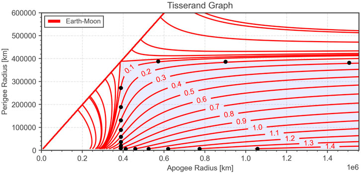
FIGURE 10. Tisserand graph showing level lines of the Jacobi integral in the Earth-Moon system with labels showing the flyby infinite velocity in km/s. The circles indicate the maximum possible travel distance achievable by a single lunar flyby with an altitude higher than 200 km.
The transfer techniques considered so far in this paper used trajectories where both the start and the end were located in a region that is dominated by either the primary or secondary body gravity. This allowed using the approximations for the Jacobi integral as expressed by Eqs 3, 4. This is not the case for so-called weak capture trajectories Schoenmaekers et al. (2001); Pernicka et al. (1994); Topputo et al. (2005); Macau (2000), which makes their treatment in the Tisserand graph a bit less generic.
This technique exploits the three body dynamics with the Earth and the Moon and in some cases allows a completely ballistic capture into a weakly bound orbit around the Moon. In any case, the capture maneuver is small (typically, a few m/s). Figure 11 shows such a capture trajectory to a southern NRHO Howell and Breakwell (1984) that has an orbital period of 6.56 days. This is the 9:2 resonant NRHO that is currently proposed as a location for the lunar Gateway Williams et al. (2017); Zimovan et al. (2017). The capture trajectory is obtained through a backwards propagation starting from the stable NRHO and applying a tangential maneuver of 15 m/s at the aposelenium. The (chronologically) initial orbit obtained is no longer bound to the Moon and can be represented in the Tisserand graph by its perigee and apogee radius. Note, however, that the inclination of this orbit is neglected at this point. It has to be matched at a later stage in the trajectory design where no longer a planar approximation is used.
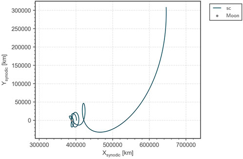
FIGURE 11. A weak capture trajectory to a southern NRHO with a period of 6.56 days obtained through backwards propagation and a capture maneuver of 15 m/s opposite to the velocity direction at aposelenium.
Figure 12 shows the points in the Tisserand graph that can be reached with this technique using 50 days of backwards propagation as a function of the capture Δv. The larger the capture maneuver, the more sensitive the initial state becomes: the Δv step used to produce Figure 12 is 2 cm/s. Obviously, the obtained points strongly depend on the sort of capture orbit that is used. Therefore, there is no generic way of visualizing weak capture trajectories in the Tisserand graph. What can be said, however, is that the starting point for a weak capture in the Tisserand graph is always around to the Jacobi level lines of the Earth-Moon libration points L1-L5, because this is energetically the region where the weak capture orbits, like the NRHO, lie.
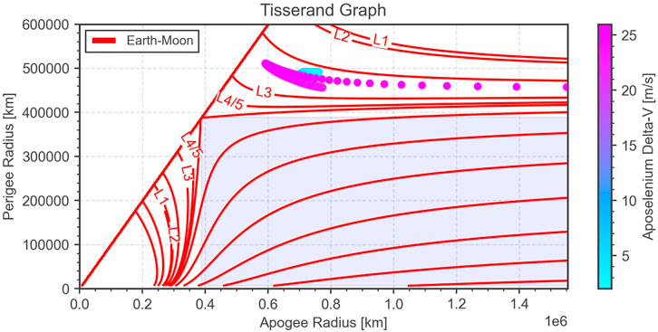
FIGURE 12. Tisserand graph showing level lines of the Jacobi integral in the Earth-Moon system. The color-coded circles indicate points from which a weak capture in an NRHO with a period of 6.56 days is achievable as a function of the capture Δv.
To make practical use of the described technique, one would choose a capture orbit and define the free parameters, like the capture Δv or the orbit orientation. A scan on these parameters is performed and the points obtained through backwards propagation are indicated in the Tisserand graph, similar to what was done in Figure 12. These points serve as target points for the trajectory design using techniques such as WSB transfers, lunar resonances and flybys. Note that for the Jupiter and Saturn systems where the mass ratio between the Moons and the planet is much lower, these target points follow much closer the level lines of the Jacobi integral than what was shown here in the Earth-Moon system Campagnola et al. (2014).
So far, mostly ballistic transfer techniques have been discussed. Maneuvers, are expected to be added once one moves past the point of initial guess generation and uses high fidelity models. However, also at the stage of initial guess generation, simple maneuvers like apogee/perigee raising/lowering can be added. These can conveniently be displayed in the Tisserand graph by horizontal (apogee raising/lowering) or vertical (perigee raising/lowering) lines. The travel distance along these lines depends on the starting point and on the applied Δv.
The real benefit of using the Tisserand graph for low-energy lunar transfer becomes apparent when a combination of the techniques discussed so far is used. Figure 13 shows two examples of such techniques.
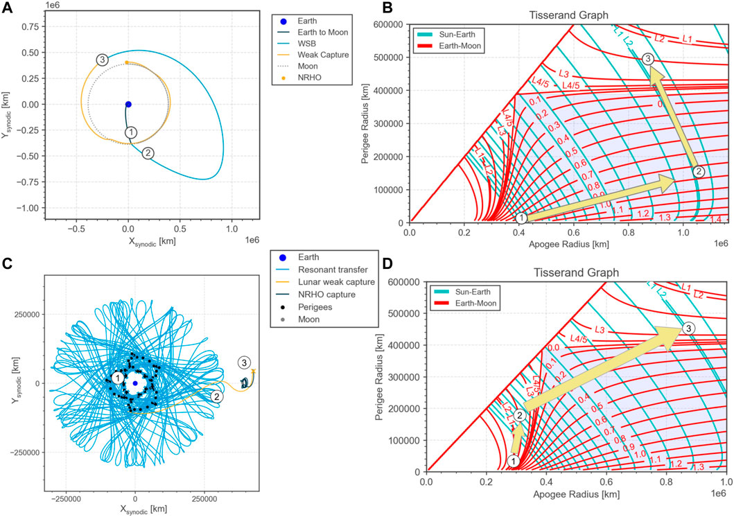
FIGURE 13. Examples of combined techniques for low-energy transfers. The plots on the top row show a transfer to NRHO using a lunar flyby, WSB transfer and weak lunar capture. The plots on the bottom row display a transfer to NRHO using a sequence of lunar resonance and weak lunar capture.
The upper part of Figures 13A,B show a trajectory that starts with a launch into a 300 × 400, 000 km orbit, performs a lunar flyby at 4,650 km altitude to increase the apogee towards the WSB region and finally uses a weak lunar capture to insert into an NRHO. The corresponding path in the Tisserand graph is shown on the upper right quadrant of the figure. The apogee raising via the lunar flyby follows the red level line of the Earth-Moon system corresponding to 860 m/s infinite velocity. The perigee raising in the WSB region follows the cyan level line close to the L2 value of the Sun-Earth Jacobi integral. The final point, 3, is one that has been identified in Section 3.4 to lead to an almost ballistic capture to NRHO using only a small insertion maneuver of 20.8 m/s.
The trajectory shown in Figure 13A was designed by first fixing points 1 and 3 in the Tisserand graph by choosing the launch orbit and by backwards propagation from the NRHO (cf. Section 3.4). Then the lunar flyby altitude and longitude of perigee were tweaked manually to find point 2 in the Tisserand graph that connects point 1 and 3 via red (lunar flyby) and cyan (WSB transfer) level lines of the Jacobi integral. The manual process was easy enough in this case, but of course this process can easily be automatized using standard root finding algorithms.
Note that the transfer shown neglects out-of-plane motion and the relative phasing between the spacecraft, the Moon and the Sun. This means that whenever the spacecraft reaches the lunar altitude, the Moon is assumed to be there. Put differently, it means that although the trajectory appears closed in space, there are time gaps at the matching points 1, 2, and 3 in Figure 13A. Techniques to close these time gaps are not covered in detail in the scope of this paper. These techniques exploit the periodicity of the individual trajectory parts of the transfer and subsequent local optimization. In particular, this implies:
• Shifting the launch date by integer Earth rotations in the Earth-Moon system.
• Shifting the lunar flyby date by integer Moon revolutions in the Sun-Earth system.
• Shifting the NRHO capture date by integer Moon revolutions in the Sun-Earth system.
These operations do not change the trajectory in space, but only alter the time gaps. Local optimization can then be used to adjust the free parameters in the system to close the time gaps and obtain a feasible trajectory from the initial guess.
As an additional example of a combined transfer, showing the different combinations achievable with the Tisserand graph, Figures 13C,D show a weak capture to NRHO, achieved with a 2.4 m/s manoeuvre, obtained after a sequence of 85 geocentric orbits, exploiting a lunar resonance to slowly raise the perigee until being captured by the lunar gravity.
The trajectory in Figure 13C was designed by first looking at the points surrounding point 3, which represent NRHO capture with different Δv values (as shown in Figure 12), then jumping back to the equivalent level line in the bottom-left quadrant of the Tisserand graph and selecting point 1 at 50,000 × 301,301 km, assuming it as departure orbit for the transfer. Point 2 is then achieved after a sequence of resonances, moving on the level line, until the “jump” to the upper-right quadrant of the Tisserand graph at the same energy level. This brings the spacecraft to the cislunar space, at the correct point for the weak capture in NRHO after the small capture manoeuvre.
As mentioned in Section 4.1, this design procedure does not take into account the phasing problem, which can be solved at a later stage with the proposed methodologies. Nevertheless, using the Tisserand graph allows for a fast initial guess design and a good insight into the problem.
The double Tisserand graph of the Earth-Moon and Sun-Earth systems is a powerful tool for designing initial guess trajectories that involve WSB transfers (Section 3.1), lunar resonance transfers (Section 3.2), lunar flybys (Section 3.3) and weak lunar captures (Section 3.4) in a circular planar model. The double Tisserand graph using generic techniques is summarized in Figure 14 for convenience. The method can be used to graphically come up with an initial guess for the sequence of apogee/perigee radii, the flyby infinite velocities, the required number of revolutions around the Earth and the optimal longitudes of perigee. Infeasible paths in the graph are easy to identify. Moreover, simple numerical solvers can be implemented in a computer program that determine the maximum step size along a level line. This allows for a fast and robust initial guess generation which can later be improved by successively moving to higher fidelity models.
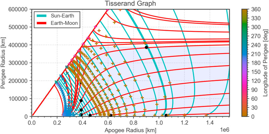
FIGURE 14. Tisserand graph showing all transfer techniques in the Sun-Earth-Moon system except weak lunar capture. Note that the longitude of perigee is defined in the Earth-Moon synodic frame for the lunar resonant transfers, but in the Sun-Earth synodic frame for the WSB transfers.
The techniques described in this paper are not only applicable to the Sun-Earth-Moon system, but also to other planetary systems, like Jupiter or Saturn. Because the mass ratio of the Moons in the gas giants is much smaller compared to the Earth-Moon system, the approximations described in this paper work much better there. They can be efficiently used for Moon tour design.
The original contributions presented in the study are included in the article/Supplementary Material, further inquiries can be directed to the corresponding author.
WM and LB contributed to the design of the study. WM carried out the analysis and derivations and wrote the draft of the manuscript. Both authors contributed to manuscript revision, read, checked and approved the submitted version.
The work presented in this article was funded by the European Space Agency.
The authors declare that the research was conducted in the absence of any commercial or financial relationships that could be construed as a potential conflict of interest.
All claims expressed in this article are solely those of the authors and do not necessarily represent those of their affiliated organizations, or those of the publisher, the editors and the reviewers. Any product that may be evaluated in this article, or claim that may be made by its manufacturer, is not guaranteed or endorsed by the publisher.
The Supplementary Material for this article can be found online at: https://www.frontiersin.org/articles/10.3389/frspt.2022.920456/full#supplementary-material
1The direction of the Sun gravity gradient can be computed from the CR3BP gravitational potential in the Sun-Earth system, but here only the general direction is relevant. It always points away from the Earth and towards the Sun-Earth line in the synodic reference frame as shown in Figure 3A
Battin, R. H. (1987). An introduction to the mathematics and methods of astrodynamics. New York: AIAA.
Belbruno, E. A., and Miller, J. K. (1993). Sun-perturbed Earth-to-moon transfers with ballistic capture. J. Guid. Control, Dyn. 16, 770–775. doi:10.2514/3.21079
Belbruno, E. (2018). Capture dynamics and chaotic motions in celestial mechanics. Princeton, NJ, USA: Princeton University Press.
Belbruno, E. (1987). “Lunar capture orbits, a method of constructing Earth moon trajectories and the lunar GAS mission,” in 19th International Electric Propulsion Conference, 1054.
Bellome, A., Cuartielles, J.-P. S., Felicetti, L., and Kemble, S. (2020). “Modified tisserand map exploration for preliminary multiple gravity assist trajectory design,” in 71st International Astronautical Congress - the Cyberspace Edition, 12-14 October 2020. Online.
Campagnola, S., Boutonnet, A., Schoenmaekers, J., Grebow, D. J., Petropoulos, A. E., Russell, R. P., et al. (2014). Tisserand-leveraging transfers. J. Guid. Control, Dyn. 37, 1202–1210. doi:10.2514/1.62369
Campagnola, S., and Russell, R. P. (2010). Endgame problem part 2: Multibody technique and the tisserand-poincaré graph. J. Guid. Control, Dyn. 33, 476–486. doi:10.2514/1.44290
de la Torre Sangrà, D., Fantino, E., Flores, R., Calvente Lozano, O., and García Estelrich, C. (2021). An automatic tree search algorithm for the tisserand graph. Alexandria Eng. J. 60, 1027–1041. doi:10.1016/j.aej.2020.10.028
Hoffman, T. L. (2009). “Grail: Gravity mapping the moon,” in 2009 IEEE Aerospace conference, 1–8. doi:10.1109/aero.2009.4839327
Howell, K., and Breakwell, J. (1984). Almost rectilinear halo orbits. Celest. Mech. 32, 29–52. doi:10.1007/BF01358402
Macau, E. E. (2000). Using chaos to guide a spacecraft to the moon. Acta Astronaut. 47, 871–878. doi:10.1016/S0094-5765(00)00125-9
Miller, J., and Weeks, C. (2002). “Application of tisserand’s criterion to the design of gravity assist trajectories,” in AIAA/AAS Astrodynamics Specialist Conference and Exhibit, 4717.
Parrish, N. L., Kayser, E., Udupa, S., Parker, J. S., Cheetham, B. W., and Davis, D. C. (2020). “Ballistic lunar transfers to near rectilinear halo orbit: Operational considerations,” in AIAA Scitech 2020 Forum, 1466.
Pernicka, H., Scarberry, D., Marsh, S., and Sweetser, T. (1994). “A search for low delta-v Earth-to-moon trajectories,” in AAS/AIAA Astrodynamics Conference, 3772.
Ross, S. D., and Scheeres, D. J. (2007). Multiple gravity assists, capture, and escape in the restricted three-body problem. SIAM J. Appl. Dyn. Syst. 6, 576–596. doi:10.1137/060663374
Schoenmaekers, J., Horas, D., and Pulido, J. (2001). “SMART-1: With solar electric propulsion to the moon,” in Proceeding of the 16th International Symposium on Space Flight Dynamics (Pasadena, CA: NASA Jet Propulsion Lab), 3–7.
Strange, N. J., and Longuski, J. M. (2002). Graphical method for gravity-assist trajectory design. J. Spacecr. Rockets 39, 9–16. doi:10.2514/2.3800
Topputo, F. (2013). On optimal two-impulse Earth–moon transfers in a four-body model. Celest. Mech. Dyn. Astron. 117, 279–313. doi:10.1007/s10569-013-9513-8
Topputo, F., Vasile, M., and Bernelli-Zazzera, F. (2005). Earth-to-moon low energy transfers targeting L1 hyperbolic transit orbits. Ann. N. Y. Acad. Sci. 1065, 55–76. doi:10.1196/annals.1370.025
Whitley, R., and Martinez, R. (2016). “Options for staging orbits in cislunar space,” in 2016 IEEE Aerospace Conference, 1–9. doi:10.1109/aero.2016.7500635
Williams, J., Lee, D. E., Whitley, R. J., Bokelmann, K. A., Davis, D. C., and Berry, C. F. (2017). “Targeting cislunar near rectilinear halo orbits for human space exploration,” in AAS/AIAA Space Flight Mechanics Meeting. JSC-CN-38615.
Yárnoz, D. G., Yam, C. H., Campagnola, S., and Kawakatsu, Y. (2016). “Extended tisserand-poincaré graph and multiple lunar swingby design with sun perturbation,” in Proceedings of the 6th International Conference on Astrodynamics Tools and Techniques.
Keywords: circular restricted three body problem, tisserand graph, weak stability boundary, low energy transfer, Moon, four body problem, lunar gateway
Citation: Martens W and Bucci L (2022) Double Tisserand graphs for low-energy lunar transfer design. Front. Space Technol. 3:920456. doi: 10.3389/frspt.2022.920456
Received: 14 April 2022; Accepted: 05 July 2022;
Published: 27 September 2022.
Edited by:
Josep Masdemont, Universitat Politecnica de Catalunya, SpainReviewed by:
Hao Peng, Rutgers, The State University of New Jersey—Busch Campus, United StatesCopyright © 2022 Martens and Bucci. This is an open-access article distributed under the terms of the Creative Commons Attribution License (CC BY). The use, distribution or reproduction in other forums is permitted, provided the original author(s) and the copyright owner(s) are credited and that the original publication in this journal is cited, in accordance with accepted academic practice. No use, distribution or reproduction is permitted which does not comply with these terms.
*Correspondence: Waldemar Martens, d2FsZGVtYXIubWFydGVuc0Blc2EuaW50
Disclaimer: All claims expressed in this article are solely those of the authors and do not necessarily represent those of their affiliated organizations, or those of the publisher, the editors and the reviewers. Any product that may be evaluated in this article or claim that may be made by its manufacturer is not guaranteed or endorsed by the publisher.
Research integrity at Frontiers
Learn more about the work of our research integrity team to safeguard the quality of each article we publish.