Formation flying along libration point orbits using chattering attenuation sliding mode control

This paper studies a control law to achieve formation flying in cislunar space. Utilizing the eigenstructure of the linearized flow around a libration point of the Earth-Moon circular restricted three-body problem, the fuel efficient formation flying controller based on the chattering attenuation sliding mode controller is designed and analyzed. Numerical studies are conducted for the Earth-Moon L₂ point and a halo orbit around it. The total velocity change required to achieve formation as well as to maintain the orbit is calculated. Simulation results show that the chattering attenuation sliding mode controller has good performance and robustness in the presence of unmodeled nonlinearity along the halo orbit with moderate fuel consumption.

1 Introduction

Cislunar space provides an attractive and long-term opportunity to open the way for future manned and unmanned deep space exploration and to bridge the gap between current and future space missions. Missions in cislunar space also play an important role in enabling the future missions to the Moon, near-Earth asteroids (NEAs), Mars, and other deep space exploration. Recently, considerable attention has been devoted to the trajectory design in cislunar space (Farquhar et al., 2004; Crusan et al., 2018, 2019; Wu et al., 2019). Since libration point orbits in cislunar space are highly unstable, a spacecraft moving on these orbits must use control input to remain close to their nominal orbits. A great variety of studies have investigated methods for stabilizing the unstable periodic orbits in the circular restricted three-body problem (CR3BP) (Gomez et al., 1998; Farquhar et al., 2004; Folta et al., 2014; Ulybyshev, 2014; Xu et al., 2016; Qian et al., 2018). Floquet mode control has been applied for stationkeeping of libration point orbits which eliminates the local unstable components by an impulsive maneuver (Simo et al., 1987). In Howell and Marchand (2005), formation flying around libration point orbits utilizing natural relative motions on center manifold was proposed by adding an impulsive maneuver to eliminate the unstable components. The idea of natural formation was generalized to a continuous control law by Scheeres et al. (2003) and it was shown that the simple feedback control law can stabilize unstable periodic orbits and create additional center manifolds. However, disturbances such as the gravitational forces of the Sun and other planets in the actual space environment, which can destabilize orbits, have not been taken into account in these methods.

Sliding mode control (SMC) has been recognized as a nonlinear robust control technique because of its inherent advantages of strong stability, disturbance rejection and low sensitivity to plant parameter variations (Utkin, 1992). For decades until now, many engineers and researchers have relied on the performance of the SMC for aerospace applications such as launch vehicles (Shtessel et al., 2000; Hall and Shtessel, 2006), formation flying in Earth orbit (Li et al., 2012), asteroid precision landing (Furfaro et al., 2013) and attitude control (Hu et al., 2013). Based on high-order sliding-mode theory, an adaptive disturbance-based sliding-mode controller for hypersonic vehicles has been introduced (Yu et al., 2015; Sun et al., 2018). Adaptive second-order sliding mode trajectory tracking control for flexible air-breathing hypersonic vehicles with measurement noises has been proposed to cope with uncertainties, disturbances and measurement noises (Sagliano et al., 2017). In Lian and Tang (2013), the rendezvous problem between libration point orbits in the Earth-Moon system was studied based on a terminal sliding mode controller with prescribed time of flight, which is the attractive feature of their proposed method. In Gong et al. (2014), SMC was applied to generate quasi-periodic and periodic orbits around the L₂ libration point in the Earth-Moon system using a solar sail.

Despite the popularity of SMC technique, SMC has a major drawback called chattering, i.e., undesired oscillations of control input. Chattering is an inevitable phenomenon due to the inherent discontinuity or switching nature around sliding surfaces. A number of approaches were developed to avoid the chattering. Continuous approximations are often used to approximate the discontinuous signum function in a boundary layer around the switching manifold. However, sliding mode performances will be compromised by introducing the boundary layer. To solve this problem while preserving the main advantages of SMC, higher-order sliding mode control (HOSM) has been proposed which generalizes the basic sliding mode idea to act on the higher-order time derivatives of the system deviation (Emel’Yanov et al., 1996; Levant, 2003; Boiko, 2014). However, real-time higher-order output derivatives are necessary to implement the HOSM, which might be difficult to obtain depending on the application. In fact, though arbitrary-order exact robust differentiators have been addressed, implementation of higher-order differentiation is not exact because of the computational limitations (Shtessel et al., 2014). Furthermore, the speed of the system’s trajectory is very slow when the states are far away from the origin in the super-twisting algorithm (STA), which is a simplest form of the second-order sliding mode technique (Moreno, 2014). Moreover, STA cannot endure uncertainties and disturbances that change with the system states (Kunusch et al., 2012). Recently, chattering attenuation sliding mode control (CASMC) was developed by Nemati et al. as a new technique to attenuate the chattering phenomena (Nemati et al., 2017). The structure of CASMC is simple, but includes a time-varying switching function that can reduce the magnitude of discontinuous functions over time.

The goal of this paper is to design a robust and fuel efficient control law for formation flying in the vicinity of a collinear libration point in the Earth-Moon system, leveraging the manifold structure of natural dynamics and robustness of SMC. In this study, the controlled state is constrained to a hyperplane with zero unstable component by sliding mode control to achieve natural formation under unmodeled nonlinearity. In particular, we show that it is possible to stabilize the unstable relative motion and generate a bounded motion by a single control input. Although SMC has the remarkable property that the response of the system remains insensitive to disturbances and/or uncertainties of models, conventional SMC presents drawbacks of chattering. Moreover, SMC requires high control authority in general. To overcome these problems, we formulate a novel SMC control law based on the chattering attenuation sliding mode control framework. The control gain is designed to reduce the cost of SMC by incorporating the linear quadratic regulator (LQR) theory. The parameters of the CASMC are chosen so that the total cost (ΔV) of CASMC is almost equal to that of LQR for the ideal case and the L₁ norm of the control input to maintain a halo orbit is examined.

The paper is organized as follows. Section 1 is the introduction. Section 2 reviews the equations of motion in the CR3BP and their state space form. Section 3 gives the stabilization of unstable mode by linear control and sliding mode control. Section 4 presents simulation results. Section 5 considers formation flying along a halo orbit by sliding mode control. Finally, Section 6 gives the conclusions.

2 Equations of motion in the CR3BP

The equations of motion of a massless spacecraft under the gravitational attraction of the Earth and Moon is considered. In the CR3BP, the Earth and Moon are assumed to move in circular orbits about their common barycenter. Consider a rotating frame in which the origin is fixed at the barycenter, the Z-axis is aligned with the angular velocity of the primaries, the X-axis is directed from the Earth to Moon, and the Y-axis completes the right-handed coordinate system. The distance between spacecraft and the Earth and Moon are respectively given by r₁ and r₂ as

$\begin{array}{ll}\hfill r_1& =\sqrt{{\left(X+\rho \right)}^2+Y^2+Z^2}\hfill \\ \hfill r_2& =\sqrt{{\left(X-1+\rho \right)}^2+Y^2+Z^2}\hfill \end{array}$

Then, the equations of motion of the CR3BP in the non-dimensional form (Wie, 2008) are given by

$\begin{array}{ll}\hfill \ddot{X}-2\dot{Y}-X& =-\frac{1-\rho }{r_1^3}\left(X+\rho \right)-\frac{\rho }{r_2^3}\left(X-1+\rho \right)+u_x\hfill \\ \hfill \ddot{Y}+2\dot{X}-Y& =-\frac{1-\rho }{r_1^3}Y-\frac{\rho }{r_2^3}Y+u_y\hfill \\ \hfill \ddot{Z}& =-\frac{1-\rho }{r_1^3}Z-\frac{\rho }{r_2^3}Z+u_z\hfill \end{array}(1)$

where ρ = M_m/(M_E + M_m), M_E and M_m are the masses of the Earth and Moon, (u_x, u_y, u_z) is the control acceleration and the equations of motion are normalized so that the distance d between the Earth and Moon and angular velocity ω are equal to one. Eq. 1 has stationary points known as Lagrangian points L_i satisfying

$\begin{array}{ll}\hfill X& =\frac{1-\rho }{r_1^3}\left(X+\rho \right)+\frac{\rho }{r_2^3}\left(X-1+\rho \right)\hfill \\ \hfill Y& =\frac{1-\rho }{r_1^3}Y+\frac{\rho }{r_2^3}Y\hfill \\ \hfill Z& =0\hfill \end{array}(2)$

and

$\begin{array}{ll}\hfill & L_1=\left(l_1\left(\rho \right),\mathrm{0,0}\right),L_2=\left(l_2\left(\rho \right),\mathrm{0,0}\right),L_3=\left(l_3\left(\rho \right),\mathrm{0,0}\right)\hfill \\ \hfill & L_4=\left(1/2-\rho ,\sqrt{3}/\mathrm{2,0}\right),L_5=\left(1/2-\rho ,-\sqrt{3}/\mathrm{2,0}\right)\hfill \end{array}$

where l_i(ρ) are determined by the first equation of Eq. 2. To describe equations of motion near a collinear equilibrium point L_i (i = 1, 2, 3), it is convenient to use the coordinate system with its center at L_i. Replacing X, Y, Z by x + l_i, y, z, Eq. 1 can be written as

$\begin{array}{ll}\hfill \ddot{x}-2\dot{y}-x& =l_i-\frac{1-\rho }{r_1^3}\left(x+l_i+\rho \right)-\frac{\rho }{r_2^3}\left(x+l_i-1+\rho \right)+u_x\hfill \\ \hfill \ddot{y}+2\dot{x}-y& =-\frac{1-\rho }{r_1^3}y-\frac{\rho }{r_2^3}y+u_y\hfill \\ \hfill \ddot{z}& =-\frac{1-\rho }{r_1^3}z-\frac{\rho }{r_2^3}z+u_z\hfill \end{array}(3)$

where

$\begin{array}{ll}\hfill r_1& =\sqrt{{\left(x+l_i+\rho \right)}^2+y^2+z^2}\hfill \\ \hfill r_2& =\sqrt{{\left(x+l_i-1+\rho \right)}^2+y^2+z^2}\hfill \end{array}$

The linearized equations of Eq. 3 at the origin are given by

$\begin{array}{ll}\hfill \ddot{x}-2\dot{y}-\left(2{\sigma }_i+1\right)x& =u_x\hfill \\ \hfill \ddot{y}+2\dot{x}+\left({\sigma }_i-1\right)y& =u_y\hfill \\ \hfill \ddot{z}+{\sigma }_{i}z& =u_z\hfill \end{array}(4)$

where

${\sigma }_i=\frac{\rho }{|l_i\left(\rho \right)-1+\rho {|}^3}+\frac{1-\rho }{|l_i\left(\rho \right)+\rho {|}^3}(5)$

The state space form of Eq. 4 is expressed as

$\dot{\mathit{x}}=A\mathit{x}+B\mathit{u}(6)$

where $\mathit{x}={[xyz\dot{x}\dot{y}\dot{z}]}^T$, $\mathit{u}={[u_x{u}_y{u}_z]}^T$, and

$A=\left[\begin{array}{cccccc}\hfill 0\hfill & \hfill 0\hfill & \hfill 0\hfill & \hfill 1\hfill & \hfill 0\hfill & \hfill 0\hfill \\ \hfill 0\hfill & \hfill 0\hfill & \hfill 0\hfill & \hfill 0\hfill & \hfill 1\hfill & \hfill 0\hfill \\ \hfill 0\hfill & \hfill 0\hfill & \hfill 0\hfill & \hfill 0\hfill & \hfill 0\hfill & \hfill 1\hfill \\ \hfill 2{\sigma }_i+1\hfill & \hfill 0\hfill & \hfill 0\hfill & \hfill 0\hfill & \hfill 2\hfill & \hfill 0\hfill \\ \hfill 0\hfill & \hfill 1-{\sigma }_i\hfill & \hfill 0\hfill & \hfill -2\hfill & \hfill 0\hfill & \hfill 0\hfill \\ \hfill 0\hfill & \hfill 0\hfill & \hfill -{\sigma }_i\hfill & \hfill 0\hfill & \hfill 0\hfill & \hfill 0\hfill \end{array}\right],B=\left[\begin{array}{ccc}\hfill 0\hfill & \hfill 0\hfill & \hfill 0\hfill \\ \hfill 0\hfill & \hfill 0\hfill & \hfill 0\hfill \\ \hfill 0\hfill & \hfill 0\hfill & \hfill 0\hfill \\ \hfill 1\hfill & \hfill 0\hfill & \hfill 0\hfill \\ \hfill 0\hfill & \hfill 1\hfill & \hfill 0\hfill \\ \hfill 0\hfill & \hfill 0\hfill & \hfill 1\hfill \end{array}\right]$

The state space form of nonlinear equations in Eq. 3 is then semilinear and is given by (Akiyama et al., 2018)

$\dot{\mathit{x}}=A\mathit{x}+B\mathit{f}\left(\mathit{x}\right)+B\mathit{u}(7)$

where

$\mathit{f}\left(\mathit{x}\right)=\left[\begin{array}{c}\hfill l_i-2{\sigma }_{i}x-\frac{1-\rho }{r_1^3}\left(x+l_i+\rho \right)-\frac{\rho }{r_2^3}\left(x+l_i-1+\rho \right)\hfill \\ \hfill {\sigma }_{i}y-\frac{1-\rho }{r_1^3}y-\frac{\rho }{r_2^3}y\hfill \\ \hfill {\sigma }_{i}z-\frac{1-\rho }{r_1^3}z-\frac{\rho }{r_2^3}z\hfill \end{array}\right]=\left[\begin{array}{c}\hfill f_x\hfill \\ \hfill f_y\hfill \\ \hfill f_z\hfill \end{array}\right],(8)$

Observe that the matrix A has two real eigenvalues and a complex conjugate eigenvalue pair. New state vector is introduced as $\mathit{z}={[z_{1c}{z}_{2c}{z}_{3c}{z}_{4c}{z}_s{z}_u]}^T=T^{-1}\mathit{x}$, where subscripts c, s and u denote center, stable and unstable modes, respectively. Then the matrix T transforms the matrix A into a real block diagonal form $\tilde{A}$ by $AT=T\tilde{A}$. The transformation matrix T and the real block diagonal form $\tilde{A}$ are given by.

$T=\left[\begin{array}{cccccc}\hfill 0\hfill & \hfill 0\hfill & \hfill -P_2\hfill & \hfill 0\hfill & \hfill -P_1\hfill & \hfill -P_1\hfill \\ \hfill 0\hfill & \hfill 0\hfill & \hfill 0\hfill & \hfill -1/Q_2\hfill & \hfill -1/Q_3\hfill & \hfill 1/Q_3\hfill \\ \hfill 1/Q_1\hfill & \hfill 0\hfill & \hfill 0\hfill & \hfill 0\hfill & \hfill 0\hfill & \hfill 0\hfill \\ \hfill 0\hfill & \hfill 0\hfill & \hfill 0\hfill & \hfill -P_2{Q}_2\hfill & \hfill P_1{Q}_3\hfill & \hfill -P_1{Q}_3\hfill \\ \hfill 0\hfill & \hfill 0\hfill & \hfill 1\hfill & \hfill 0\hfill & \hfill 1\hfill & \hfill 1\hfill \\ \hfill 0\hfill & \hfill 1\hfill & \hfill 0\hfill & \hfill 0\hfill & \hfill 0\hfill & \hfill 0\hfill \end{array}\right],(9)$

$\tilde{A}=\left[\begin{array}{cccccc}\hfill 0\hfill & \hfill Q_1\hfill & \hfill 0\hfill & \hfill 0\hfill & \hfill 0\hfill & \hfill 0\hfill \\ \hfill -Q_1\hfill & \hfill 0\hfill & \hfill 0\hfill & \hfill 0\hfill & \hfill 0\hfill & \hfill 0\hfill \\ \hfill 0\hfill & \hfill 0\hfill & \hfill 0\hfill & \hfill Q_2\hfill & \hfill 0\hfill & \hfill 0\hfill \\ \hfill 0\hfill & \hfill 0\hfill & \hfill -Q_2\hfill & \hfill 0\hfill & \hfill 0\hfill & \hfill 0\hfill \\ \hfill 0\hfill & \hfill 0\hfill & \hfill 0\hfill & \hfill 0\hfill & \hfill -Q_3\hfill & \hfill 0\hfill \\ \hfill 0\hfill & \hfill 0\hfill & \hfill 0\hfill & \hfill 0\hfill & \hfill 0\hfill & \hfill Q_3\hfill \end{array}\right](10)$

Where

$\begin{array}{llll}\hfill Q_1& =\sqrt{{\sigma }_i}\hfill & \hfill P_1& =\frac{4}{4+3{\sigma }_i-\sqrt{{\sigma }_i}\sqrt{-8+9{\sigma }_i}}\hfill \\ \hfill Q_2& =\sqrt{\frac{\left.2-{\sigma }_i+\sqrt{{\sigma }_i}\sqrt{-8+9{\sigma }_i}\right)}{2}}\hfill & \hfill P_2& =\frac{4}{4+3{\sigma }_i+\sqrt{{\sigma }_i}\sqrt{-8+9{\sigma }_i}}\hfill \\ \hfill Q_3& =\sqrt{\frac{-2+{\sigma }_i+\sqrt{{\sigma }_i}\sqrt{-8+9{\sigma }_i}}{2}}\hfill & \hfill \end{array}(11)$

are positive constants. The state space form [Eq. 6] becomes in the new state variables as

$\dot{\mathit{z}}=\tilde{A}\mathit{z}+\tilde{B}\mathit{u}(12)$

where

$\tilde{B}=T^{-1}B=\left[\begin{array}{ccc}\hfill 0\hfill & \hfill 0\hfill & \hfill 0\hfill \\ \hfill 0\hfill & \hfill 0\hfill & \hfill 1\hfill \\ \hfill 0\hfill & \hfill \frac{P_1}{P_1-P_2}\hfill & \hfill 0\hfill \\ \hfill -\frac{Q_2}{P_2{Q_2}^2+P_1{Q_3}^2}\hfill & \hfill 0\hfill & \hfill 0\hfill \\ \hfill \frac{Q_3}{2\left(P_2{Q_2}^2+P_1{Q_3}^2\right)}\hfill & \hfill -\frac{P_2}{2\left(P_1-P_2\right)}\hfill & \hfill 0\hfill \\ \hfill -\frac{Q_3}{2\left(P_2{Q_2}^2+P_1{Q_3}^2\right)}\hfill & \hfill -\frac{P_2}{2\left(P_1-P_2\right)}\hfill & \hfill 0\hfill \end{array}\right](13)$

Also, the semilinear form [Eq. 7] is rewritten as

$\dot{\mathit{z}}=\tilde{A}\mathit{z}+\tilde{B}\mathit{f}\left(T\mathit{z}\right)+\tilde{B}\mathit{u}(14)$

where

$T\mathit{z}=\mathit{x}=\left[\begin{array}{c}\hfill -P_2{z}_{3c}-P_1\left(z_s+z_u\right)\hfill \\ \hfill -\frac{1}{Q_2}{z}_{4c}-\frac{1}{Q_3}\left(z_s-z_u\right)\hfill \\ \hfill \frac{z_{1c}}{Q_1}\hfill \\ \hfill -P_2{Q}_2{z}_{4c}+P_1{Q}_3\left(z_s-z_u\right)\hfill \\ \hfill z_{3c}+z_s+z_u\hfill \\ \hfill z_{2c}\hfill \end{array}\right](15)$

Consequently, the equations of motion can be rewritten in the new variables as.

${\dot{z}}_{1c}=Q_1{z}_{2c}(16)$

${\dot{z}}_{2c}=-Q_1{z}_{1c}+f_z+u_z(17)$

${\dot{z}}_{3c}=Q_2{z}_{4c}+\frac{P_1}{P_1-P_2}\left(f_y+u_y\right)(18)$

${\dot{z}}_{4c}=-Q_2{z}_{3c}-\frac{Q_2}{P_2{Q_2}^2+P_1{Q_3}^2}\left(f_x+u_x\right)(19)$

${\dot{z}}_s=-Q_3{z}_s+\frac{Q_3}{2\left(P_2{Q_2}^2+P_1{Q_3}^2\right)}\left(f_x+u_x\right)-\frac{P_2}{2\left(P_1-P_2\right)}\left(f_y+u_y\right)(20)$

${\dot{z}}_u=Q_3{z}_u-\frac{Q_3}{2\left(P_2{Q_2}^2+P_1{Q_3}^2\right)}\left(f_x+u_x\right)-\frac{P_2}{2\left(P_1-P_2\right)}\left(f_y+u_y\right)(21)$

In the following, we construct a controller to place the spacecraft in the center manifold of the libration point based on Eqs 16–21, then it is generalized to formation flying along a periodic orbit. Although control input affects both stable and unstable manifolds, we can design a controller to stabilize unstable manifold while stable and center manifolds are preserved, owing to the explicit form of Eqs 16–21. As a result, a spacecraft will naturally circulate about the periodic orbit in three-dimensional space.

3 Stabilization of unstable mode by linear and nonlinear control

For simplicity, stabilization of the in-plane motion is discussed based on the new state variables since the in-plane and out-of-plane motions of the linearized system (Eq. 12) are independent. Motivated by the fact that eliminating the unstable mode and the use of the center manifold is enough to achieve stable formation flying (Scheeres et al., 2003; Howell and Marchand, 2005), this section studies feedback controllers based on reduced-order system.

3.1 Stabilization of unstable mode by linear control

The in-plane motion of linearized equation (Eq. 12) can be rewritten by the following two state equations:

${\dot{\mathit{z}}}_1={\tilde{A}}_1{\mathit{z}}_{\mathbf{1}}+{\tilde{B}}_1{\mathit{u}}_{in}(22)$

${\dot{\mathit{z}}}_2={\tilde{A}}_2{\mathit{z}}_{\mathbf{2}}+{\tilde{B}}_2{\mathit{u}}_{in}(23)$

where

$\begin{array}{llllll}\hfill {\mathit{z}}_{\mathbf{1}}& =\left[\begin{array}{c}\hfill z_{3c}\hfill \\ \hfill z_{4c}\hfill \end{array}\right],\hfill & \hfill {\mathit{z}}_{\mathbf{2}}& =\left[\begin{array}{c}\hfill z_s\hfill \\ \hfill z_u\hfill \end{array}\right],\hfill & \hfill {\mathit{u}}_{in}& =\left[\begin{array}{c}\hfill u_x\hfill \\ \hfill u_y\hfill \end{array}\right]\hfill \\ \hfill {\tilde{A}}_1& =\left[\begin{array}{cc}\hfill 0\hfill & \hfill Q_2\hfill \\ \hfill -Q_2\hfill & \hfill 0\hfill \end{array}\right],\hfill & \hfill {\tilde{A}}_2& =\left[\begin{array}{cc}\hfill -Q_3\hfill & \hfill 0\hfill \\ \hfill 0\hfill & \hfill Q_3\hfill \end{array}\right]\hfill & \hfill \\ \hfill {\tilde{B}}_1& =\left[\begin{array}{cc}\hfill 0\hfill & \hfill \frac{P_1}{P_1-P_2}\hfill \\ \hfill -\frac{Q_2}{P_2{Q_2}^2+P_1{Q_3}^2}\hfill & \hfill 0\hfill \end{array}\right],\hfill & \hfill {\tilde{B}}_2& =\frac{1}{2}\left[\begin{array}{cc}\hfill \frac{Q_3}{P_2{Q_2}^2+P_1{Q_3}^2}\hfill & \hfill -\frac{P_2}{P_1-P_2}\hfill \\ \hfill -\frac{Q_3}{P_2{Q_2}^2+P_1{Q_3}^2}\hfill & \hfill -\frac{P_2}{P_1-P_2}\hfill \end{array}\right]\hfill & \hfill \end{array}$

Based on Eq. 23, the feedback controllers are designed and the stability of the whole system should be verified through Eqs 22, 23. In the following, three approaches are shown: 1) using only u_x (referred to as “u_x-controller”), 2) using only u_y (referred to as “u_y-controller”), and 3) using the combination of u_x and u_y (referred to as “(u_x, u_y)-controller”).

3.2 Stabilizing the unstable mode by single input

Since both u_x and u_y affect the unstable manifold in Eq. 21, we first assume u_y = 0 for simplicity and u_x is designed to stabilize the system shown in Eqs 22, 23. Applying u_x = k_xz_u to Eq. 21 yields

${\dot{z}}_u=Q_3\left[1-\frac{k_x}{2\left(P_2{Q_2}^2+P_1{Q_3}^2\right)}\right]z_u(24)$

Therefore, if $k_x>2\left(P_2{Q_2}^2+P_1{Q_3}^2\right)$, then Eq. 24 is asymptotically stable, i.e. z_u → 0 as t → ∞. On the other hand, Eq. 22 becomes

$\left[\begin{array}{c}\hfill {\dot{z}}_{3c}\hfill \\ \hfill {\dot{z}}_{4c}\hfill \end{array}\right]=\left[\begin{array}{cc}\hfill 0\hfill & \hfill Q_2\hfill \\ \hfill -Q_2\hfill & \hfill 0\hfill \end{array}\right]\left[\begin{array}{c}\hfill z_{3c}\hfill \\ \hfill z_{4c}\hfill \end{array}\right]-\left[\begin{array}{c}\hfill 0\hfill \\ \hfill \frac{k_x{Q}_2}{P_2{Q_2}^2+P_1{Q_3}^2}\hfill \end{array}\right]z_u(25)$

Then from Eq. 25, z_3c and z_4c are bounded because z_u → 0 as t → ∞. The stability of z_s can be verified by,

${\dot{z}}_s=-Q_3{z}_s+\frac{Q_3{k}_x}{2\left(P_2{Q_2}^2+P_1{Q_3}^2\right)}{z}_u(26)$

From Eq. 26, z_s is asymptotically stable since z_u → 0 as t → ∞. Therefore, the whole system Eqs 22, 23 is stable in the Lyapunov sense. In a similar way, we can choose the feedback control as u_y = k_yz_u with u_x = 0.

3.3 Stabilizing the unstable mode by a combination of u_x and u_y

There exists another option to stabilize the unstable mode where u_x and u_y are chosen as

$\frac{Q_3}{P_2{Q_2}^2+P_1{Q_3}^2}{u}_x=\frac{P_2}{P_1-P_2}{u}_y(27)$

In this case, no control input is added to the stable mode z_s. A feedback control is designed to satisfy Eq. 27 as.

$u_x=k_{xy}{z}_u(28)$

$u_y=\frac{Q_3\left(P_1-P_2\right)}{P_2\left(P_2{Q}_2^2+P_1{Q}_3^2\right)}{u}_x=\frac{Q_3\left(P_1-P_2\right)}{P_2\left(P_2{Q}_2^2+P_1{Q}_3^2\right)}{k}_{xy}{z}_u(29)$

To summarize the three approaches, the following controllers are derived:

(u_x = k_xz_u with u_y = 0) where

$k_x>2\left(P_2{Q_2}^2+P_1{Q_3}^2\right)(30)$

(u_y = k_yz_u with u_x = 0) where

$k_y>2Q_3\left(\frac{P_1}{P_2}-1\right)(31)$

(u_x = k_xyz_u and u_y = Cu_x) where

$k_{xy}>P_2{Q_2}^2+P_1{Q_3}^2,C=\frac{Q_3\left(P_1-P_2\right)}{P_2\left(P_2{Q}_2^2+P_1{Q}_3^2\right)}(32)$

Since the system ($\tilde{A}$, $\tilde{B}$) is controllable, a feedback control law can be designed by the pole placement technique. Consider the generalized feedback control of the form for Eqs 22, 23:

${\mathit{u}}_{in}=K_1{\mathit{z}}_1+K_2{\mathit{z}}_2(33)$

Then, the control laws Eqs 30–32 can be considered as a special case of the pole placement where the unstable eigenvalue is moved to left-half plane while other eigenvalues are not changed, i.e. K₁ = 0. It is observed that the first term K₁z₁ of Eq. 33 can only change the pole locations of Eq. 22 while those of Eq. 23 are not affected. Therefore, any K₁ such that ${\tilde{A}}_1+{\tilde{B}}_1{K}_1$ has eigenvalues on the imaginary axis would change the center mode to other center mode. Moreover, Eq. 22 is stabilized by any feedback control K₂z₂ such that ${\tilde{A}}_2+{\tilde{B}}_2{K}_2\le 0$. Note that Scheeres et al. (2003) considers only the special case where ${\tilde{A}}_2+{\tilde{B}}_2{K}_2$ has eigenvalues on the imaginary axis.

3.4 Stabilization by sliding mode control

In this section, one of robust control techniques called sliding mode control (SMC), which is a particular type of variable structure control, is introduced to deal with nonlinearities and uncertainties of the CR3BP. SMC design generally proceeds in two steps. The first step is to design a switching manifold such that the system’s states are restricted to the sliding surface and hence, those states can be ensured to reach the desired dynamics. The second step is to design a robust control law to drive the states to the switching manifold and maintain them on the sliding surface based on the Lyapunov stability approach. The simple sliding manifold for the first-order system is expressed as

$S=\lambda \left(z_{u,d}-z_u\right)(34)$

where S is the switching manifold, z_u,d is a desired response for z_u and λ is a positive constant. For example, the desired response z_u,d can be chosen as

${\dot{z}}_{u,d}=-{\sigma }^2{z}_{u,d}(35)$

It should be noted that the parameter λ is typically limited by three factors: the frequency of the lowest unmodeled structural resonant mode ν_R, the largest neglected time delay T_d, and the sampling rate ν_s as follows (Slotine and Li, 1991):

$\lambda \le \frac{2\pi }{3}{\nu }_R,\lambda \le \frac{1}{3T_d},\lambda \le \frac{1}{5}{\nu }_s(36)$

In the following, the u_x-controller is designed by a conventional SMC approach as an example. The SMC for the other type of controllers described in Section 3.1 are designed in the same manner. Consider the Lyapunov candidate as

$V=\frac{1}{2}{S}^2(37)$

where S is the sliding manifold described by Eq. 34. The time derivative of Eq. 37 along the solution of Eq. 21 is given by

$\dot{V}=S\dot{S}=S\left\{\lambda {\dot{z}}_{u,d}-\lambda \left[Q_3{z}_u-\frac{Q_3}{2\left(P_2{Q_2}^2+P_1{Q_3}^2\right)}{\tilde{u}}_x-\frac{P_2}{2\left(P_1-P_2\right)}{f}_y\right]\right\}(38)$

where ${\tilde{u}}_x=f_x+u_x$. To guarantee the asymptotic stability, the time derivative of the Lyapunov function should be negative, i.e.,

$\dot{V}=-\mu |S|(39)$

where the parameter μ is a strictly positive constant and should be greater than the magnitude of the disturbance (see Appendix A). Substituting Eq. 39 into Eq. 38 yields

$\dot{S}=-\mu \text{sign}\left(S\right)(40)$

where sign(S) is a signum function defined as follows:

$\text{sign}\left(S\right)=\frac{|S|}{S}=\left\{\begin{array}{cc}1\hfill & S>0\hfill \\ 0\hfill & S=0\hfill \\ -1\hfill & S<0\hfill \end{array}\right.(41)$

From Eqs 38, 40, we have

$Q_3{z}_u-\frac{Q_3}{2\left(P_2{Q_2}^2+P_1{Q_3}^2\right)}{\tilde{u}}_x-\frac{P_2}{2\left(P_1-P_2\right)}{f}_y={\dot{z}}_{u,d}+\frac{\mu }{\lambda }\text{sign}\left(S\right).(42)$

By substituting ${\tilde{u}}_x=f_x+u_x$ into Eq. 42, u_x can be found as

$u_x=\frac{2\left(P_2{Q_2}^2+P_1{Q_3}^2\right)}{Q_3}\left[Q_3{z}_u-{\dot{z}}_{u,d}-\frac{P_2}{2\left(P_1-P_2\right)}{f}_y-\frac{\mu }{\lambda }\text{sign}\left(S\right)\right]-f_x(43)$

Note that the feedback gain of z_u in Eq. 43 is specified as $2\left(P_2{Q_2}^2+P_1{Q_3}^2\right)$ by the constants in Eq. 11. The stability of the whole system [Eqs. 22, 23 can be verified in the same manners as in Section 3.1. Since the state reaches the switching manifold in a finite time and is kept on the manifold, the value of sliding surface becomes zero (S = 0) theoretically. However, in real applications, states are not kept on the switching manifold exactly. The signum function [Eq. 41] switches the control signal at a high but finite frequency, and thereby excites the unmodeled fast dynamics or undesirable oscillations called chattering, although it contributes the insensitivity to disturbances and model uncertainties. Chattering can deteriorate system performance, and even lead to instability.

Hereby, without violating the sliding condition, an improved SMC strategy called the chattering attenuation sliding mode control (CASMC) (Nemati et al., 2017) is introduced to alleviate the magnitude of the discontinuous function over time. Typically, the chattering attenuation sliding manifold of CASMC is defined as

$S_{\mathit{CASMC}}=\lambda e^{at+b}\left(z_{u,d}-z_u\right)(44)$

where a and b are positive constants which are designed under the conditions of Nemati and Hokamoto (2014). This procedure is illustrated for the specific problem of CR3BP in Section 4.2. Consequently, the chattering attenuation sliding control law is obtained as

$u_{x,CASMC}=\frac{2\left(P_2{Q_2}^2+P_1{Q_3}^2\right)}{Q_3}\left[\left(Q_3+a\right)z_u-{\dot{z}}_{u,d}-a{z}_{u,d}-\frac{P_2}{2\left(P_1-P_2\right)}{f}_y-\frac{\mu }{\lambda e^{at+b}}\text{sign}\left(S\right)\right]-f_x(45)$

It can be seen that the magnitude of signum function is $\frac{\mu }{\lambda e^{at+b}}$ while $\frac{\mu }{\lambda }$ for the conventional SMC. Therefore, the trade-off between chattering attenuation and robustness can be regulated by two parameters a and b. Furthermore, the feedback gain of z_u is replaced by $\frac{2\left(P_2{Q_2}^2+P_1{Q_3}^2\right)}{Q_3}(Q_3+a)$, which is a function of a. This property is also used to reduce the L₁ norm of the control input in Section 4.2. The u_y-controller can be designed in a similar way as

$u_{y,CASMC}=2\frac{P_1-P_2}{P_2}\left[\left(Q_3+a\right)z_u-{\dot{z}}_{u,d}-a{z}_{u,d}-\frac{Q_3}{2\left(P_2{Q_2}^2+P_1{Q_3}^2\right)}{f}_x-\frac{\mu }{\lambda e^{at+b}}\text{sign}\left(S\right)\right]-f_y(46)$

Similarly, (u_x, u_y)-controller is given by.

$u_{x,CASMC}=\frac{P_2{Q_2}^2+P_1{Q_3}^2}{Q_3}\left[\left(Q_3+a\right)z_u-{\dot{z}}_{u,d}-a{z}_{u,d}-\frac{P_2}{2\left(P_1-P_2\right)}{f}_y-\frac{\mu }{\lambda e^{at+b}}\text{sign}\left(S\right)\right]-\frac{1}{2}{f}_x(47)$

$u_{y,CASMC}=C\left(u_{x,CASMC}+\frac{1}{2}{f}_x\right)-\frac{1}{2}{f}_y(48)$

Note that the stable mode z_s naturally converges to zero as time goes to infinity by single input CASMC. However, to guarantee fast convergence of the stable mode, the multi-input CASMC can be designed. To design multi-input CASMC, two independent sliding manifolds are selected as

$S_{1,CASMC}={\lambda }_1{e}^{a_{1}t+b_1}\left(z_{s,d}-z_s\right)(49)$

$S_{2,CASMC}={\lambda }_2{e}^{a_{2}t+b_2}\left(z_{u,d}-z_u\right)(50)$

Then, the u_x- and u_y-controllers for the multi-input CASMC are obtained similarly as

$\begin{array}{ll}\hfill u_{x,2-CASMC}& =\frac{P_2{Q_2}^2+P_1{Q_3}^2}{Q_3}\left[Q_3\left(z_u+z_s\right)+\frac{{\mu }_1}{{\lambda }_1{e}^{a_{1}t+b_1}}\text{sign}\left(S_{1,CASMC}\right)-{\dot{z}}_{u,d}+{\dot{z}}_{s,d}\right.\hfill \\ \hfill & \left.-\frac{{\mu }_2}{{\lambda }_2{e}^{a_{2}t+b_2}}\text{sign}\left(S_{2,CASMC}\right)+a_1\left(z_{s,d}-z_s\right)-a_2\left(z_{u,d}-z_u\right)\right]-f_x\hfill \end{array}(51)$

$\begin{array}{ll}\hfill u_{y,2-CASMC}& =\frac{P_1-P_2}{P_2}\left[Q_3\left(z_u-z_s\right)-\frac{{\mu }_1}{{\lambda }_1{e}^{a_{1}t+b_1}}\text{sign}\left(S_{1,CASMC}\right)-{\dot{z}}_{u,d}-{\dot{z}}_{s,d}\right.\hfill \\ \hfill & \left.-\frac{{\mu }_2}{{\lambda }_2{e}^{a_{2}t+b_2}}\text{sign}\left(S_{2,CASMC}\right)-a_1\left(z_{s,d}-z_s\right)-a_2\left(z_{u,d}-z_u\right)\right]-f_y\hfill \end{array}(52)$

4 Numerical simulations

In order to validate and compare the L₁ norms of the proposed controllers, the Earth-Moon L₂ point is considered. The parameters of the Earth-Moon CR3BP are shown in Table 1. Here, no control input for the out-of-plane motion (z − axis) is assumed, i.e. u_z = 0 because the out-of-plane motion is decoupled in the linearized system [Eq. 6].

TABLE 1

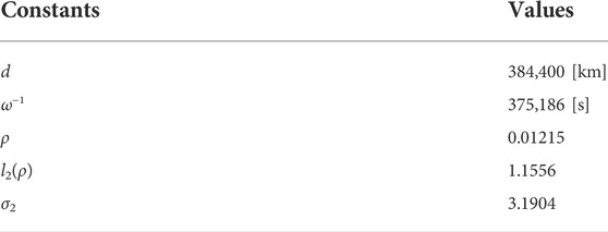
TABLE 1. Parameters of the earth-moon CR3BP.

4.1 Eliminating unstable mode by feedback controllers

As a preliminary analysis, feedback controllers are designed by the linear quadratic regulator (LQR) theory to minimize the L₁ norm of the control input $\left({\int }_{t_0}^{t_f}|u|dt\right)$. The feedback gain is given by

$K=-R^{-1}{B}^{T}P(53)$

where the matrix P is the solution to the algebraic Riccati equation (ARE):

$A^{T}P+PA-PB{R}^{-1}{B}^{T}P+Q=0(54)$

$Q=\mathbb{I}$, $R=10^r\mathbb{I}$ ($\mathbb{I}$ is an identity matrix) and r is a scalar parameter. It is known that the L₂ norm (square integral) of control input converges monotonically to its minimum value as Q decreases to zero, or equivalently as R increases to infinity (Bando and Ichikawa, 2013). However, the required total velocity change (ΔV) is represented by the L₁ norm of the control input. Thus, the L₁ norms of the proposed controllers are investigated. In the numerical simulations, the linear feedback is applied to the nonlinear equation [Eq. 1] and the L₁ norm for five periods is computed.

The three types of controllers described in Section 3 (u_x-, u_y-, and (u_x, u_y)-controller) are designed by ARE. When u_x-controller is used, Eq. 54 is reduced to a scalar equation

$2Q_{3}p-\frac{p^2}{r}{\left(\frac{Q_3}{2\left(P_2{Q}_2^2+P_1{Q}_3^2\right)}\right)}^2+q=0(55)$

where q = 1, and the stabilizing feedback is explicitly given by

$u_x=k_x{z}_u=-\left[2\left(P_2{Q}_2^2+P_1{Q}_3^2\right)+\frac{\sqrt{4{\left(P_2{Q}_2^2+P_1{Q}_3^2\right)}^2{r}^2+r}}{r}\right]z_u(56)$

Similarly, u_y-controller and (u_x, u_y)-controller are respectively given by

$u_y=k_y{z}_u=-\left[\frac{2Q_3\left(P_1-P_2\right)}{P_2}+\frac{\sqrt{4Q_3^2{r}^2{\left(P_1-P_2\right)}^2+r{P}_2^2}}{P_{2}r}\right]z_u(57)$

and.

$u_x=k_{xy}{z}_u=-\left[\left(P_2{Q}_2^2+P_1{Q}_3^2\right)+\frac{\sqrt{{\left(P_2{Q}_2^2+P_1{Q}_3^2\right)}^2{r}^2+r}}{r}\right]z_u(58)$

$u_y=\frac{Q_3\left(P_1-P_2\right)}{P_2\left(P_2{Q}_2^2+P_1{Q}_3^2\right)}{u}_x(59)$

By these controllers, stabilization of the unstable mode is realized.

Figure 1 demonstrates the controlled trajectory by u_x-, u_y- and (u_x, u_y)-controllers. It can be seen that the trajectory of spacecraft becomes a quasi-periodic orbit which encloses the L₂ point by eliminating the unstable mode. As being consistent to the analytical result in Sec. 3, it can be said that the in-plane motion can be controlled by a single control input u_x or u_y.

FIGURE 1

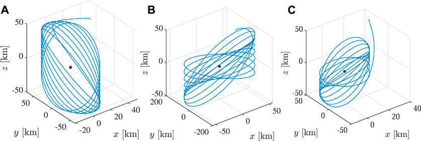
FIGURE 1. Controlled trajectory by u_x-controller [x₀, y₀, z₀] = [38, 38, 38] km, r = −4. (A) u_x-controller, (B) u_y-controller, (C) (u_x, u_y)-controller.

From Eqs 56–58, it is clear that when r → ∞ the limit of the feedback gains exist and are given by.

$\underset{r\to \infty }{\lim }{k}_x=-4\left(P_2{Q}_2^2+P_1{Q}_3^2\right)\approx -16.2586(60)$

$\underset{r\to \infty }{\lim }{k}_y=-4\frac{Q_3\left(P_1-P_2\right)}{P_2}\approx -25.7974(61)$

$\underset{r\to \infty }{\lim }{k}_{xy}=-2\left(P_2{Q}_2^2+P_1{Q}_3^2\right)\approx -8.12932(62)$

Therefore, the L₁ norms of the control input saturates for large r.

The L₁ norms for each LQR controller for various r are summarized in Figure 2. It is found that the L₁ norms for r ≥ −9 are reduced by u_x- and (u_x, u_y)-controllers compared to u_y-controller. The L₁ norms of u_x-controller and (u_x, u_y)-controller are almost half of that of u_y-controller for large r. This can be explained by Eq. 21 as that u_x has more impact than u_y since the coefficient of u_x is almost double of that of u_y. Moreover, it is worth noting that the L₁ norm of u_x-controller is almost the same as (u_x, u_y)-controller although an extra control effort is added to the stable mode.

FIGURE 2

FIGURE 2. L₁ norm vs. r based on LQR.

4.2 Chattering attenuation sliding mode controllers

The CASMC is designed to validate the practical implementation of SMC. The CASMC is employed because it has a simple structure with sufficient robustness. For simplicity, z_u,d ≡ 0 is considered so that the state on the sliding manifold is restricted to the stable and center subspaces. The CASMC can affect the robust performance of the system because in general, there is a delicate balance between chattering attenuation and robustness as described in Appendix A. However, compared with other methods to eliminate chattering (e.g., using continuous approximations such as a sigmoid function, a hyperbolic function, etc (Khalil, 2002)), the CASMC somewhat preserves robustness because chattering phenomenon will not be completely eliminated or replaced by a continuous approximation, but it will be suppressed over time. In the following, the same parameters λ = 0.01 and μ = 0.02 are used for CASMC.

To preserve the robustness over time, a saturating function f(t) as shown in Figure 3 is employed such that the term $\frac{1}{f(t)}$ numerically suppresses the chattering effect and simultaneously preserves the robustness. The saturating chattering attenuation function is given by

$f\left(t\right)=\left\{\begin{array}{cc}{e}^{at+b}\hfill & t\le t^{\ast }\hfill \\ F\hfill & t>t^{\ast }\hfill \end{array}\right.(63)$

where t* is a specified time and F is the upper bound of the chattering attenuation function. The parameter t* determines the length of the interval where the effect of chattering attenuation remains. If we choose t∗ to be larger than a settling time T_s, then the chattering can be sufficiently attenuated but the robustness decreases. However, if large disturbance exists, we have to choose t∗ < T_s to maintain robustness though the chattering might remain more than expected.

FIGURE 3

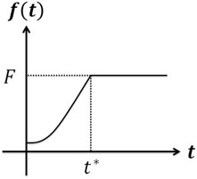
FIGURE 3. Schematic of a chattering attenuation function.

In the following, the CASMC parameters a, b and F are designed for the Earth-Moon CR3BP. Since the CASMC has the linear feedback term which is a function of the parameter a in Eqs 45, 46, the parameter a affects the L₁ norm as the parameter r in LQR. Therefore, the parameter a corresponding to a sufficiently large r is chosen to ensure the small L₁ norm. On the other hand, the upper bound of the chattering attenuation function F is important to suppress the chattering over time. To design F, one may employ a settling time T_s as a saturation condition for t∗ in Eq. 63, that is, the parameter F can be designed as

$f\left(T_s\right)=e^{a{T}_s+b}=F(64)$

Figure 4 shows the histories of the control input and state variables by the CASMC u_x-controller with different parameters a, which correspond to −3 ≤ r ≤ 6. The controlled trajectory of spacecraft becomes a quasi-periodic orbit with different periods which encloses the L₂ point by eliminating the unstable mode. It can be seen that chattering is sufficiently suppressed and that the magnitude of control input is very small $(<3.5\times 10^{-9})$ in Figure 4A. Next, the parameter b is determined from the robust performance as well as chattering suppression at initial phase. From the robustness condition [Eq. 78] at t = 0, the parameter b should satisfy $b\le \ln \frac{\mu }{\lambda D}$. Practically, the magnitude of the maximum amplitude of the disturbance D should be taken into account to satisfy $0<b\le \ln \frac{\mu }{\lambda D}$, however, this condition is relaxed in many cases as can be seen in the following results. Here, b = 13 is chosen by that the value of the signum function is reduced by e⁻¹³ = 2.26 × 10^–6. The settling time which is determined by the stopping rule |z_u| ≤ 10^–10 is T_s = 1.13 [day] which corresponds to 0.2626 in nondimensional time unit, therefore F = 1.7614 × 10⁸ is obtained from Eq. 64. From the robustness condition [Eq. 78], the maximum amplitude of disturbances or uncertainties to guarantee the stability is given by $D=\frac{\mu }{\lambda F}=1.1354\times 10^{-8}$ in nondimensional unit. Figure 5 summarizes the result of CASMC for −3 ≤ a ≤ 6 and b = 20 based on u_x- and u_y-controllers. The figure shows that the cost of CASMC is almost the same as that of LQR.

FIGURE 4

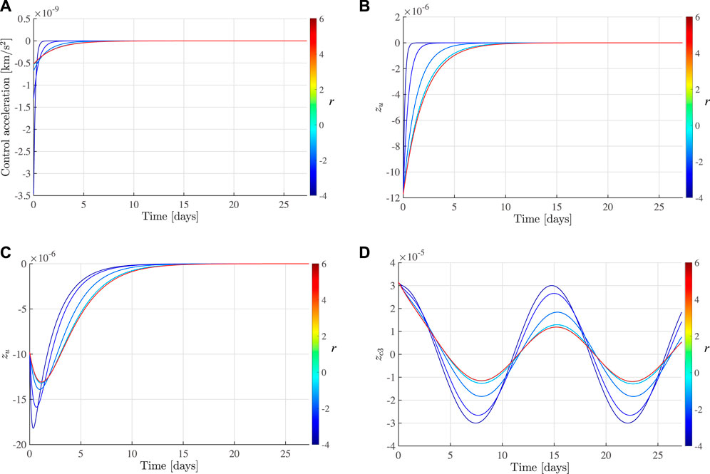
FIGURE 4. Controlled trajectory by CASMC ux-controller. (A) Control history, (B) $z_u$, (C) $z_s$, (D) $z_{c3{$.

FIGURE 5

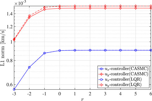
FIGURE 5. L₁ norm vs. r based on CASMC.

The maximum accelerations shown in Figure 4A vary between 3.47 × 10^–9 ≤ u_max ≤ 5.20, ×, 10^–10 [km/s²]. These value are compatible with recent or proposed low-thrust missions such as Deep Space 1, Dawn, Gateway and Lunar IceCube mission (Rayman et al., 2000; Russell and Raymond, 2012; McCarty et al., 2018; Pritchett et al., 2019). For example, the low-thrust capability of Dawn is 7.473 × 10^–8 [km/s²] which is larger than the maximum thrust magnitude of the proposed controller. Moreover, the solar gravitational perturbation is compatible with the proposed thrust magnitude level which is the largest perturbation in cislunar environment. Other perturbations such as the gravitational attraction and the ephemeris of the planets, the presence of solar radiation pressure and orbit determination errors are also considered as an unmodeled dynamics in the CR3BP. Figure 9 summarizes the result of CASMC u_x-controller for formation flying.

5 Formation flying along halo orbit

5.1 Derivation of relative dynamics

To maintain the halo orbit, which is denoted by x_f, a standard way is to linearize Eq. 7 along x_f and apply the target method or a linear feedback theory for periodic systems (Howell and Henry, 1993; Folta and Vaughn, 2004; Bando and Ichikawa, 2014; Bando and Scheeres, 2016). In Bando and Ichikawa (2014), a simple feedback control for station-keeping is proposed based on the semilinear form Eq. 7. The advantage of this approach is that the control law does not require the computation of the state transition matrix along the reference halo orbit. In this section, the semilinear form described by the new variable [Eq. 14] is used instead of the semilinear form Eq. 7, which makes it possible to take into account the eigenstructure of the libration point for the fuel efficient trajectory design.

Let z_f be a periodic orbit of the leader near the L_i point given by

${\dot{\mathit{z}}}_f=\tilde{A}{\mathit{z}}_f+\tilde{B}f\left(T{\mathit{z}}_f\right)(65)$

where ${\mathit{z}}_f={[z_{\mathit{1cf}}{z}_{\mathit{2cf}}{z}_{\mathit{3cf}}{z}_{\mathit{4cf}}{z}_{sf}{z}_{uf}]}^T$. Let z be the controlled trajectory of the follower given by

$\dot{\mathit{z}}=\tilde{A}\mathit{z}+\tilde{B}f\left(T\mathit{z}\right)+\tilde{B}\mathit{u}(66)$

where $\mathit{z}={[z_{1c}{z}_{2c}{z}_{3c}{z}_{4c}{z}_s{z}_u]}^T$ and u is control input. Then, the error system is given by

$\dot{\mathit{e}}=\tilde{A}\mathit{e}+\tilde{B}\left(f\left(T\mathit{z}\right)-f\left(T{\mathit{z}}_f\right)\right)+\tilde{B}\mathit{u}(67)$

where $\mathit{e}=\mathit{z}-{\mathit{z}}_f={[e_{1c}{e}_{2c}{e}_{3c}{e}_{4c}{e}_s{e}_u]}^T$. The semilinear form (67) is reduced to the linearized equation

$\dot{\mathit{e}}=\tilde{A}\mathit{e}+\tilde{B}\mathit{u}(68)$

if |f (Tz) − f (Tz_f)| is sufficiently small. Observe that Eq. 68 has the same structure as Eq. 12. Therefore, the follower can achieve natural formation around the leader’s orbit by elliminating the unstable mode with the controllers designed for the libration points in Section 3 where the nonlinear term |f (Tz) − f (Tz_f)| can be considered as an unmodeled nonlinearity.

5.2 Formation flying along halo orbit by sliding mode control

The parameters of the Earth-Moon CR3BP in Section 4 are used in this section. A particular halo orbit around L₂ is given by the normalized initial condition

${\mathit{x}}_{f0}={\left[1.17760.0000-0.05500.0000-0.17120.0000\right]}^T(69)$

and its period is T = 3.3904 (≈14.7226 [day]). The initial position of the follower at time t₀ (= 0) is assumed to be

${\mathit{x}}_0={\mathit{x}}_f\left(0\right)+\mathit{e}\left(0\right)(70)$

where e (0) = 10^–5 × [1.0 1.0 1.0 0.0 0.0 0.0]^T (≈38.44 [km]) represents the initial offset. For the parameters a, b and F of CASMC, the same values are used as in the libration point case.

Figure 6 shows the controlled trajectory for 10 revolutions (10T = 33.904) by the single input CASMC (u_x-controller is used here). It should be noted that the larger initial deviation (≈384 [km]) is used to exaggerate the result in this figure since the deviation of 38.44 km is too small to distinguish from the reference halo orbit. Figure 7 shows the relative trajectory with respect to the reference halo orbit. Figure 8 shows the results by the CASMC u_x-controller with different parameters a, which correspond to −3 ≤ r ≤ 6. It is confirmed in Figure 8A that the chattering does not occur and the magnitude of control is sufficiently small. Compared to the results in Sec.4, deviations in unstable error components e_u exist for the formation flying case. Moreover, for a large r, which corresponds to a smaller gain, the deviation of unstable element becomes larger. This is because the nonlinear term acts the system as a time-varying unmodeled nonlinearity shown in Figure 8B and cause a large deviation in the stable error components e_s. Even though the deviations exist, the bounded relative motion along the halo orbit is achieved for −3 ≤ r ≤ 6. The center components (e_1c, e_2c, e_3c, e_4c) constitute quasi-periodic motions in Figures 8E,F. Simulation results show that the proposed sliding mode controller has good performance in the presence of unmodeled nonlinearity along the halo orbit with relatively small stationkeeping cost. In fact, the maximum accelerations shown in Figure 8A vary between 3.24 × 10^–10 ≤ u_max ≤ 2.19, ×, 10^–9 [km/s²]. These value are compatible with recent or proposed low-thrust missions.

FIGURE 6

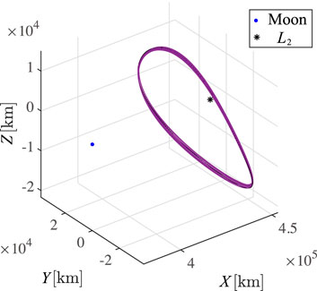
FIGURE 6. Controlled trajectory by CASMC u_x-controller (large initial deviation [δx₀, δy₀, δz₀] = [384, 384, 384] km is used to exaggerate the result in this figure).

FIGURE 7

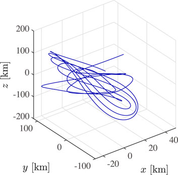
FIGURE 7. Relative motion with respect to halo orbit.

FIGURE 8

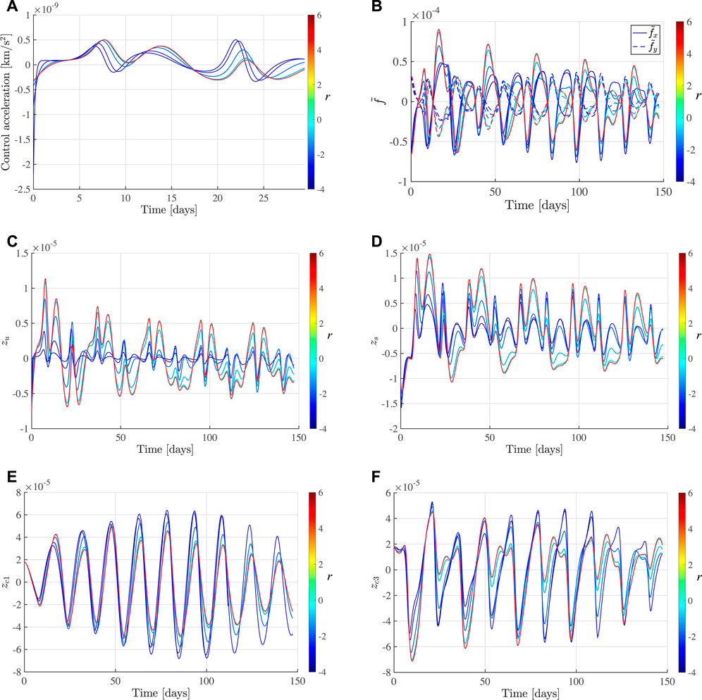
FIGURE 8. Relative trajectory generated by CASMC ux-controller for 10 revolution. (A) Control history, (B) Nonlinear terms, (C) $z_u$, (D) $z_s$, (E) $z_{c1{$, (F) $z_{c3{$.

FIGURE 9

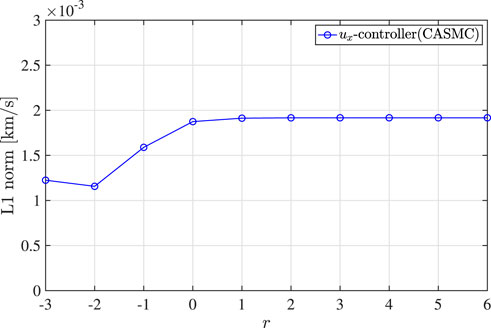
FIGURE 9. L₁ norm vs. r based on CASMC.

6 Conclusion

This paper studies the control law to stabilize the orbital motion in the vicinity of an unstable equilibrium point and periodic orbits in the circular restricted three-body problem. First, it was shown that the single input controller can stabilize the unstable mode to generate a bounded motion. Three types of controllers were derived and their stability conditions were given. Then, the chattering attenuation sliding mode controller was designed to attenuate chattering and reduce control costs at the same time based on the optimal gain computed by linear quadratic regulator. The performance of the proposed controller was tested on the Earth-Moon L₂ point and the halo orbit in the vicinity of L₂ point. It was revealed that the total velocity change is the smaller along the x-axis. Then, the proposed controller was applied to the relative motion with respect to a halo orbit. The proposed sliding mode controller can stabilize the error dynamics along a halo orbit in the presence of unmodeled nonlinearity. Moreover, the fuel expenditure of the chattering attenuation sliding mode controller is moderate and the chattering phenomena are suppressed by selecting the reasonable value for design parameters. The proposed controller is powerful and easy to implement, hence formation flying proposed in this paper is useful for the implementation in actual missions.

Data availability statement

The original contributions presented in the study are included in the article/Supplementary Material, further inquiries can be directed to the corresponding author.

Author contributions

The work was conceptualized and developed as a collaboration among all authors. The manuscript was drafted by MB, and the authors HN, YA, and SH revised the manuscript.

Funding

The work of the second author was partially supported by JSPS KAKENHI Grant Number JP21K18781.

Conflict of interest

The authors declare that the research was conducted in the absence of any commercial or financial relationships that could be construed as a potential conflict of interest.

Publisher’s note

All claims expressed in this article are solely those of the authors and do not necessarily represent those of their affiliated organizations, or those of the publisher, the editors and the reviewers. Any product that may be evaluated in this article, or claim that may be made by its manufacturer, is not guaranteed or endorsed by the publisher.

References

Akiyama, Y., Bando, M., and Hokamoto, S. (2018). Explicit form of station-keeping and formation flying controller for libration point orbits. J. Guid. Control, Dyn. 41, 1407–1415. doi:10.2514/1.G002845

CrossRef Full Text | Google Scholar

Bando, M., and Ichikawa, A. (2014). Formation flying along halo orbit of circular-restricted three-body problem. J. Guid. Control, Dyn. 38, 123–129. doi:10.2514/1.g000463

CrossRef Full Text | Google Scholar

Bando, M., and Ichikawa, A. (2013). In-plane motion control of hill–clohessy–wiltshire equations by single input. J. Guid. Control, Dyn. 36, 1512–1522. doi:10.2514/1.57197

CrossRef Full Text | Google Scholar

Bando, M., and Scheeres, D. J. (2016). Attractive sets to unstable orbits using optimal feedback control. J. Guid. Control, Dyn. 39, 2725–2739. doi:10.2514/1.g000524

CrossRef Full Text | Google Scholar

Boiko, I. M. (2014). On relative degree, chattering and fractal nature of parasitic dynamics in sliding mode control. J. Frankl. Inst. 351, 1939–1952. doi:10.1016/j.jfranklin.2013.01.003

CrossRef Full Text | Google Scholar

Crusan, J., Bleacher, J., Caram, J., Craig, D., Goodliff, K., Herrmann, N., et al. (2019). NASA’s gateway: an update on progress and plans for extending human presence to cislunar space. IEEE Aerosp. Conf. (IEEE) 1–19.

PubMed Abstract | Google Scholar

Crusan, J. C., Smith, R. M., Craig, D. A., Caram, J. M., Guidi, J., Gates, M., et al. (2018). Deep space gateway concept: extending human presence into cislunar space. IEEE Aerosp. Conf. (IEEE). 1–10.

CrossRef Full Text | Google Scholar

Emel’Yanov, S., Korovin, S., and Levant, A. (1996). High-order sliding modes in control systems. Comput. Math. Model. 7, 294–318. doi:10.1007/bf01128162

CrossRef Full Text | Google Scholar

Farquhar, R. W., Dunham, D. W., Guo, Y., and McAdams, J. V. (2004). Utilization of libration points for human exploration in the sun–earth–moon system and beyond. Acta Astronaut. 55, 687–700. doi:10.1016/j.actaastro.2004.05.021

CrossRef Full Text | Google Scholar

Folta, D. C., Pavlak, T. A., Haapala, A. F., Howell, K. C., and Woodard, M. A. (2014). Earth–moon libration point orbit stationkeeping: theory, modeling, and operations. Acta Astronaut. 94, 421–433. doi:10.1016/j.actaastro.2013.01.022

CrossRef Full Text | Google Scholar

Folta, D., and Vaughn, F. (2004). “A survey of earth-moon libration orbits: stationkeeping strategies and intra-orbit transfers,” in AIAA/AAS astrodynamics specialist conference and exhibit, Reston, VA, 4741.

CrossRef Full Text | Google Scholar

Furfaro, R., Cersosimo, D., and Wibben, D. R. (2013). Asteroid precision landing via multiple sliding surfaces guidance techniques. J. Guid. Control, Dyn. 36, 1075–1092. doi:10.2514/1.58246

CrossRef Full Text | Google Scholar

Gong, S., Li, J., and Simo, J. (2014). Orbital motions of a solar sail around the L₂ earth–moon libration point. J. Guid. Control, Dyn. 37, 1349–1356. doi:10.2514/1.g000063

CrossRef Full Text | Google Scholar

Gomez, G., Howell, K., Masdemont, J., and Simo, C. (1998). Station-keeping strategies for translunar libration point orbits. Adv. Astronautical Sci. 99, 949

Google Scholar

Hall, C. E., and Shtessel, Y. B. (2006). Sliding mode disturbance observer-based control for a reusable launch vehicle. J. Guid. control, Dyn. 29, 1315–1328. doi:10.2514/1.20151

CrossRef Full Text | Google Scholar

Howell, K. C., and Marchand, B. G. (2005). Natural and non-natural spacecraft formations near the L₁ and L₂ libration points in the Sun–Earth/Moon ephemeris system. Dyn. Syst. 20, 149–173. doi:10.1080/1468936042000298224

CrossRef Full Text | Google Scholar

Howell, K., and Henry, J. (1993). Station-keeping method for libration point trajectories. J. Guid. Control, Dyn. 16, 151–159. doi:10.2514/3.11440

CrossRef Full Text | Google Scholar

Hu, Q., Xiao, B., Wang, D., and Poh, E. K. (2013). Attitude control of spacecraft with actuator uncertainty. J. Guid. Control, Dyn. 36, 1771–1776. doi:10.2514/1.58624

CrossRef Full Text | Google Scholar

Khalil, H. K. (2002). Nonlinear systems. third edition, 115. Patience Hall.

Google Scholar

Kunusch, C., Puleston, P., and Mayoski, M. (2012). Sliding-mode control of PEM fuel cells. New York: Springer.

Google Scholar

Levant, A. (2003). Higher-order sliding modes, differentiation and output-feedback control. Int. J. Control 76, 924–941. doi:10.1080/0020717031000099029

CrossRef Full Text | Google Scholar

Li, J., Pan, Y., and Kumar, K. D. (2012). Design of asymptotic second-order sliding mode control for satellite formation flying. J. Guid. control, Dyn. 35, 309–316. doi:10.2514/1.55747

CrossRef Full Text | Google Scholar

Lian, Y., and Tang, G. (2013). Libration point orbit rendezvous using PWPF modulated terminal sliding mode control. Adv. Space Res. 52, 2156–2167. doi:10.1016/j.asr.2013.08.034

CrossRef Full Text | Google Scholar

McCarty, S. L., Burke, L. M., and McGuire, M. L. (2018). “Analysis of cislunar transfers from a near rectilinear halo orbit with high power solar electric propulsion,” in AIAA astrodynamics specialist conference 2018, Reston, VA. GRC-E-DAA-TN59586, .

Google Scholar

Moreno, J. A. (2014). On strict Lyapunov functions for some non-homogeneous super-twisting algorithms. J. Frankl. Inst. 351, 1902–1919. doi:10.1016/j.jfranklin.2013.09.019

CrossRef Full Text | Google Scholar

Nemati, H., Bando, M., and Hokamoto, S. (2017). Chattering attenuation sliding mode approach for nonlinear systems. Asian J. control 19, 1519–1531. doi:10.1002/asjc.1477

CrossRef Full Text | Google Scholar

Nemati, H., and Hokamoto, S. (2014). Design procedure of chattering attenuation sliding mode attitude control of a satellite system. Adv. Astronautical Sci. 152, 3533–3541.

Google Scholar

Pritchett, R., Howell, K. C., and Folta, D. C. (2019). “Low-thrust trajectory design for a cislunar cubesat leveraging structures from the bicircular restricted four-body problem,” in International astronautical congress. GSFC-E-DAA-TN73884-1.

Google Scholar

Qian, Y., Liu, Y., Zhang, W., Yang, X., and Yao, M. (2018). Stationkeeping strategy for quasi-periodic orbit around earth–moon L₂ point. Proc. Institution Mech. Eng. Part G J. Aerosp. Eng. 230, 760–775. doi:10.1177/0954410015597257

CrossRef Full Text | Google Scholar

Rayman, M. D., Varghese, P., Lehman, D. H., and Livesay, L. L. (2000). Results from the deep space 1 technology validation mission. Acta Astronaut. 47, 475–487. doi:10.1016/s0094-5765(00)00087-4

CrossRef Full Text | Google Scholar

Russell, C., and Raymond, C. (2012). The Dawn mission to minor planets 4 vesta and 1 ceres. New York: Springer Science & Business Media.

Google Scholar

Sagliano, M., Mooij, E., and Theil, S. (2017). Adaptive disturbance-based high-order sliding-mode control for hypersonic-entry vehicles. J. Guid. Control, Dyn. 40, 521–536. doi:10.2514/1.g000675

CrossRef Full Text | Google Scholar

Scheeres, D., Hsiao, F., and Vinh, N. (2003). Stabilizing motion relative to an unstable orbit: applications to spacecraft formation flight. J. Guid. Control, Dyn. 26, 62–73. doi:10.2514/2.5015

CrossRef Full Text | Google Scholar

Shtessel, Y., Edwards, C., Fridman, L., Levant, A., et al. (2014). Sliding mode control and observation, 10. Springer.

Google Scholar

Shtessel, Y., Hall, C., and Jackson, M. (2000). Reusable launch vehicle control in multiple-time-scale sliding modes. J. Guid. Control, Dyn. 23, 1013–1020. doi:10.2514/2.4669

CrossRef Full Text | Google Scholar

Simo, C., Gomez, G., Llibre, J., Matinez, R., and Rodriguez, J. (1987). On the optimal station keeping control of halo orbits. Acta Astronaut. 15, 391–397. doi:10.1016/0094-5765(87)90175-5

CrossRef Full Text | Google Scholar

Slotine, J.-J. E., Li, W., et al. (1991). Applied nonlinear control, 199. Englewood cliffs, NJ: Prentice-Hall.

Google Scholar

Sun, J., Yi, J., Tan, X., and Pu, Z. (2018). “Robust chattering-free control for flexible air-breathing hypersonic vehicles in the presence of disturbances and measurement noises,” in 2018 annual American control conference (Milwaukee: ACC), 2264. –2269.

CrossRef Full Text | Google Scholar

Ulybyshev, Y. (2014). Long-term station keeping of space station in lunar halo orbits. J. Guid. Control, Dyn. 38, 1063–1070. doi:10.2514/1.G000242

CrossRef Full Text | Google Scholar

Utkin, V. I. (1992). Sliding modes in control and optimization. Springer-Verlag.

Google Scholar

Wie, B. (2008). Space vehicle dynamics and control. Second Edition. AIAA.

Google Scholar

Wu, W., Li, C., Zuo, L., Zhang, H., Liu, J., Wen, W., et al. (2019). Lunar farside to be explored by chang’e-4. Nat. Geosci. 12, 222–223. doi:10.1038/s41561-019-0341-7

CrossRef Full Text | Google Scholar

Xu, M., Liang, Y., and Ren, K. (2016). Survey on advances in orbital dynamics and control for libration point orbits. Prog. Aerosp. Sci. 82, 24–35. doi:10.1016/j.paerosci.2015.12.005

CrossRef Full Text | Google Scholar

Yu, P., Shtessel, Y. B., and Edwards, C. (2015). “Adaptive continuous higher order sliding mode control of air breathing hypersonic missile for maximum target penetration,” in AIAA guidance, navigation, and control conference, Reston, VA.

CrossRef Full Text | Google Scholar

7 Appendix A: Robustness analysis of the SMC and the CASMC

The robust performance of SMC is analyzed by applying matched disturbances. A nonlinear dynamical system with disturbance or parameter uncertainty can be described as follows:

$\dot{x}=g\left(x\right)+h\left(x\right)u+d\left(x,t\right)(71)$

where x represents the system’s state, g(x) and h(x) ≠ 0 are two nonlinear functions describing system dynamics, u is the control input, and d (x, t) denotes the matched disturbances or uncertainties that are unknown but bounded as d (x, t) < D. Taking the time − derivative of the Lyapunov candidate given by Eq. 37 along the uncertain system described by Eq. 71, yields

$\begin{array}{ll}\hfill \dot{V}& =S\left(\lambda \dot{x}\right)\hfill \\ \hfill & =S\lambda \left(g\left(x\right)+h\left(x\right)u+d\left(x,t\right)\right)\hfill \end{array}(72)$

Eq. 72 can be rewritten using Eq. 40 in the form of

$S\lambda \left(g\left(x\right)+h\left(x\right)u+d\left(x,t\right)\right)\le S\lambda \left(-\mu \text{sign}\left(S\right)+D\right)(73)$

Therefore, if the condition

$\mu \ge D(74)$

is satisfied, then $\dot{V}<0$ and the asymptotic stability of (71) is guaranteed.

The robust performance of CASMC can be evaluated by defining the following Lyapunov candidate:

$V=\frac{1}{2}{S_{\mathit{CASMC}}}^2(75)$

Differentiating Eq. 75 with respect to time along the uncertain system, Eq. 71, leads to

$\begin{array}{ll}\hfill \dot{V}& =S_{\mathit{CASMC}}\left[\dot{f}\left(t\right)S_{\mathit{CASMC}}+f\left(t\right)\left(\lambda \dot{x}\right)\right]\hfill \\ \hfill & =S_{\mathit{CASMC}}\left[\dot{f}\left(t\right)S_{\mathit{CASMC}}+f\left(t\right)\lambda \left(g\left(x,\dot{x}\right)+h\left(x,\dot{x}\right)u+d\left(x,t\right)\right)\right]\hfill \end{array}(76)$

Thus, substitution of Eq. 40 into Eq. 76 results in

$\begin{array}{c}\hfill \dot{f}\left(t\right)S_{\mathit{CASMC}}+f\left(t\right)\lambda \left(g\left(x,\dot{x}\right)+h\left(x,\dot{x}\right)u+d\left(x,t\right)\right)\le -\mu \text{sign}\left(S_{\mathit{CASMC}}\right)+f\left(t\right)\lambda D\end{array}(77)$

Clearly, for assuring the Lyapunov stability, the following condition must be satisfied.

$\mu \ge |f\left(t\right)|\lambda D(78)$

Eventually, Eq. 78 proves that the robust performance of the proposed chattering attenuation technique can be reduced over time. This is a crucial aspect of any methods employed chattering reduction tends to diminish the robust performance. In other words, there is a direct trade-off between chattering attenuation and robustness.