Constant-Beamwidth Kronecker Product Beamforming With Nonuniform Planar Arrays

In this paper, we address the problem of constant-beamwidth beamforming using nonuniform planar arrays. We propose two techniques for designing planar beamformers that can maintain different beamwidths in the XZ and YZ planes based on constant-beamwidth linear arrays. In the first technique, we utilize Kronecker product beamforming to find the weights, thus eliminating matrix inversion. The second technique provides a closed-form solution that allows for a tradeoff between white noise gain and directivity factor. The second technique is applicable even when only a subset of the sensors is used. Since our techniques are based on linear arrays, we also consider symmetric linear arrays. We present a method that determines where sensors should be placed to maximize the directivity and increase the frequency range over which the beamwidth remains constant, with a minimal number of sensors. Simulations demonstrate the advantages of the proposed design methods compared to the state-of-the-art. Specifically, our method yields a 1000-fold faster runtime than the competing method, while improving the wideband directivity factor by over 8 dB without compromising the wideband white noise gain in the simulated scenario.

1 Introduction

Speech, wireless communications, and radar are among the fields that use broadband beamforming (Van Veen and Buckley, 1988; Van Trees, 2004; Cohen et al., 2009). A broadband array is desirable since audible speech covers a wide range of frequencies (Snow, 1931). A constant beamwidth prevents distortion of the speech signal when the speaker moves away from the center of the mainlobe. If the beamformer weights are consistent versus frequency, the beamwidth narrows as the frequency increases (Ward et al., 1995). Therefore, the beamformer weights should be frequency-dependent to enable control of the beamwidth. Nevertheless, the sensor positions set bounds on the maximum and minimum frequency that can attain the desired beamwidth. A beamformer’s directivity is an indicator of its performance in various scenarios, such as reverberant environments. The purpose of our research is to design, with low computational complexity and a minimal number of sensors, a beamformer whose weights and positions are chosen to maximize the directivity while maintaining a constant beamwidth.

To calculate the weights for a frequency-invariant beamformer, several methods utilized the inverse Fourier transform (Ward et al., 1995, 2001; Liu and Weiss, 2004; Liu et al., 2007; Liu and Weiss, 2008; Pal and Vaidyanathan, 2010; Weiss et al., 2017), while others opted to defining an optimization problem. For simple objectives and constraints, closed form solutions were found (Parra, 2006; Zhao et al., 2009; Crocco and Trucco, 2011; Tourbabin et al., 2012; Zhao and Liu, 2012; Huang et al., 2020b), while others resorted to using optimization toolboxes (Gazor and Grenier, 1995; Yan and Ma, 2005; Chan and Chen, 2006; Yan, 2006; Zhao et al., 2008; Yan et al., 2010; Zhu and Wu, 2011; Yin, 2012; Liu et al., 2015; Li et al., 2017; Buchris et al., 2018; Liu et al., 2018; Yang X. et al., 2019; Liu et al., 2021; Son, 2021) and even deep learning methods (Aroudi and Braun, 2021; Ramezanpour et al., 2022). Recently, the Kronecker product has been utilized for beamforming to decompose the beamformer design problem into smaller problems (Yang W. et al., 2019; Benesty et al., 2019; Cohen et al., 2019; Itzhak et al., 2019; Wang et al., 2019; Huang et al., 2020a; Huang et al., 2020c; Sharma et al., 2020; Wang et al., 2020; Yang et al., 2020; Itzhak et al., 2021; Kuhn et al., 2021; Wang et al., 2021), yet it has not been applied for constant-beamwidth beamforming.

Most frequency-invariant beamformers were designed for uniform linear arrays (ULA) (Liu and Weiss, 2004; Liu et al., 2007; Liu and Weiss, 2008; Zhao et al., 2008, 2009; Liu and Weiss, 2010; Haupt and Moosbrugger, 2012; Zhao and Liu, 2012; Li et al., 2017; Rosen et al., 2017; Weiss et al., 2017; Yang X. et al., 2019; Long et al., 2019; Huang et al., 2020b; Erokhin et al., 2020; Liu et al., 2021), yet some were also developed for linear arrays (Ward et al., 1998; Parra, 2006; Pal and Vaidyanathan, 2010; Crocco and Trucco, 2011; Liu et al., 2015, 2018; Son, 2021), logarithmically spaced arrays (Ward et al., 2001), circular arrays (Chan and Chen, 2006; Yan et al., 2010; Buchris et al., 2020; Sharma et al., 2021a; Sharma et al., 2021b; Kleiman et al., 2021), and arbitrary geometry arrays (Ward et al., 1995; Yan and Ma, 2005; Yan, 2006; Zhu and Wu, 2011; Tourbabin et al., 2012; Yin, 2012). Different geometries yield varying performances. Therefore, choosing where to position the sensors has been addressed in (Gazor and Grenier, 1995; Liu et al., 2015; Buchris et al., 2018; Liu et al., 2018; Son, 2021) to maximize performance measures such as white noise gain (WNG). However, these methods require intensive computations. To alleviate the complexity of designing a two-dimensional (2D) array, we show how a constant beamwidth can be attained based on designing one-dimensional (1D) arrays. We introduce two different techniques. The first one utilizes Kronecker product properties, whereas the second technique uses a matrix transform to convert the linear array weights into planar array weights. With the second technique, we can tradeoff between WNG and directivity even when removing some sensors.

The beamwidth in the XZ plane may differ from the beamwidth in the YZ plane. This can be accomplished by designing two linear arrays, each with a different beamwidth. We position the planar array sensors based on the positions of the linear array sensors. We transform the weights used for the linear arrays to get weights for the planar beamformer. The transform ensures that the beamwidth remains constant in the XZ and YZ planes. The proposed techniques enable constant-beamwidth beamforming using planar arrays with many sensors by designing simpler linear arrays. Our design generalizes the window-based technique introduced by Long et al. (Long et al., 2019) for symmetric nonuniform linear arrays. Allowing nonuniform spacing between sensors generates additional degrees of freedom, which enables maximizing the directivity while maintaining a constant beamwidth over a broader range of frequencies. The beamformer weights are designed to take full advantage of the nonuniform interelement spacing of the symmetric array. Compared to existing methods, our generalization improves the directivity and attains a constant beamwidth over a broader range of frequencies, even for ULAs. We present two different procedures for choosing the symmetric linear array sensor positions. The first procedure is computationally intensive and involves iteratively updating the sensor positions. The purpose of this procedure is to find an upper bound on the achievable performance. Afterward, we present the second procedure that is computationally simple while maintaining on-par performance. Simulations demonstrate the properties, low design complexity, and superior performance of our design. To facilitate reproducibility, our code is available online¹.

The paper is structured as follows: Section 2 describes the signal model, performance measures, and the problem formulation. Section 3 presents beamformers for planar array geometries based on beamformers designed for linear arrays. In Section 4, we develop algorithms for finding optimal placements of the sensors for a symmetric linear array geometry and optimal design of the beamforming weights. Section 5 contains simulations and experimental results, and Section 6 concludes.

2 Signal Model and Problem Formulation

2.1 Signal Model

Consider a nonuniform planar array whose sensors are positioned on an M × N grid where the x-coordinates are ${\{x_m\}}_{m=1}^M$ and the y-coordinates are ${\{y_n\}}_{n=1}^N$. The sensor at (m, n) = (1, 1) is referred to as the reference sensor. We assume a far-field scenario, where a plane wave propagates in an anechoic environment at the speed of sound in the air, v = 343 m/s. Its direction of arrival is parameterized by the azimuth angle φ, 0° ≤ φ ≤ 360°, and elevation angle θ, 0° ≤ θ ≤ 180°. In the frequency domain, the observed signal at frequency f can be written in vector form as

$\mathbf{y}\left(f\right)=\mathbf{a}\left(f,{\phi }_{\text{d}},{\theta }_{\text{d}}\right)X\left(f\right)+\mathbf{q}\left(f\right),(1)$

where X(f) is the source signal arriving from the direction (φ_d, θ_d), q(f) is the additive noise vector of length MN, and a (f, φ, θ) is the steering vector of length MN whose entries are given by

$e^{-\mathcal{J}\frac{2\pi f}{v}\left[{\mathit{x}}_{\mathit{m}}\cos \left(\phi \right)\sin \left(\theta \right)+y_n\sin \left(\phi \right)\sin \left(\theta \right)\right]};1\le m\le M,1\le n\le N;(2)$

where $\mathcal{J}=\sqrt{‐1}$.

The beamformer output is given by

$Z\left(f\right)={\mathbf{h}}^H\left(f\right)\mathbf{y}\left(f\right),(3)$

where $\mathbf{h}\left(f\right)$ is the beamforming weight vector of length MN and ^H denotes conjugate transpose. A frequency-invariant gain is desired in the direction (φ_d, θ_d). Therefore, we impose the common distortionless constraint:

${\mathbf{h}}^H\left(f\right)\mathbf{a}\left(f,{\phi }_{\text{d}},{\theta }_{\text{d}}\right)=1.(4)$

The beampattern expresses the response of the beamformer to a plane wave and is defined as

$\mathcal{B}\left(f,\phi ,\theta ,\mathbf{h}\left(f\right)\right)={\mathbf{a}}^H\left(f,\phi ,\theta \right)\mathbf{h}\left(f\right).(5)$

To improve readability, we sometimes use a more concise notation for the steering vector, a, beamforming weight vector, h, and beampattern, $\mathcal{B}(\mathbf{h})$, by omitting the variables f, φ, and θ.

2.2 Performance Measures

We now develop wideband performance measures to quantify the WNG and directivity over a frequency band. The narrowband and wideband input signal-to-noise ratios (SNR) are

$\mathrm{i}\mathrm{S}\mathrm{N}\mathrm{R}\left(f\right)=\frac{{\varphi }_X\left(f\right)}{{\varphi }_{Q_0}\left(f\right)}(6)$

and

$\mathrm{i}\mathrm{S}\mathrm{N}\mathrm{R}=\frac{{\int }_f{\varphi }_X\left(f\right)df}{{\int }_f{\varphi }_{Q_0}\left(f\right)df},(7)$

respectively, where ${\varphi }_X\left(f\right)$ is the variance of $X\left(f\right)$ and ${\varphi }_{Q_0}\left(f\right)$ is the variance of the additive noise at the reference sensor. From (1) and (3), the narrowband and wideband output SNRs are

$\begin{array}{ll}\hfill \mathrm{o}\mathrm{S}\mathrm{N}\mathrm{R}\left(f\right)& =\frac{{\varphi }_X\left(f\right){\left|{\mathbf{h}}^H\left(f\right)\mathbf{a}\left(f,{\phi }_{\text{d}},{\theta }_{\text{d}}\right)\right|}^2}{{\mathbf{h}}^H\left(f\right){\mathbf{\Phi }}_{\mathbf{q}}\left(f\right)\mathbf{h}\left(f\right)}\hfill \\ \hfill & {=}_{\left(4\right)}\frac{{\varphi }_X\left(f\right)}{{\mathbf{h}}^H\left(f\right){\mathbf{\Phi }}_{\mathbf{q}}\left(f\right)\mathbf{h}\left(f\right)}\hfill \end{array}(8)$

and

$\begin{array}{ll}\hfill \mathrm{o}\mathrm{S}\mathrm{N}\mathrm{R}& =\frac{{\int }_f{\varphi }_X\left(f\right){\left|{\mathbf{h}}^H\left(f\right)\mathbf{a}\left(f,{\phi }_{\text{d}},{\theta }_{\text{d}}\right)\right|}^{2}df}{{\int }_f{\mathbf{h}}^H\left(f\right){\mathbf{\Phi }}_{\mathbf{q}}\left(f\right)\mathbf{h}\left(f\right)df}\hfill \\ \hfill & {=}_{\left(4\right)}\frac{{\int }_f{\varphi }_X\left(f\right)df}{{\int }_f{\mathbf{h}}^H\left(f\right){\mathbf{\Phi }}_{\mathbf{q}}\left(f\right)\mathbf{h}\left(f\right)df},\hfill \end{array}(9)$

respectively, where ${\mathbf{\Phi }}_{\mathbf{q}}\left(f\right)$ is the correlation matrix of $\mathbf{q}\left(f\right)$. The narrowband and wideband array gains are given by

$\mathcal{G}\left(f\right)=\frac{\mathrm{o}\mathrm{S}\mathrm{N}\mathrm{R}\left(f\right)}{\mathrm{i}\mathrm{S}\mathrm{N}\mathrm{R}\left(f\right)}(10)$

and

$\mathcal{G}=\frac{\mathrm{o}\mathrm{S}\mathrm{N}\mathrm{R}}{\mathrm{i}\mathrm{S}\mathrm{N}\mathrm{R}},(11)$

respectively.

When $\mathbf{q}\left(f\right)$ is spherically isotropic noise, ${\mathbf{\Phi }}_{\mathbf{q}}\left(f\right)$ is given by

${\mathbf{\Phi }}_{\mathbf{q}}\left(f\right)={\varphi }_{Q_0}\left(f\right){\mathbf{\Gamma }}_{\text{d}}\left(f\right),(12)$

where the elements of ${\mathbf{\Gamma }}_{\text{d}}\left(f\right)$ are given by

${\left[{\mathbf{\Gamma }}_{\text{d}}\left(f\right)\right]}_{r,r^{\prime }}=\mathrm{s}\mathrm{i}\mathrm{n}\mathrm{c}\left(\frac{2\pi f}{v}{d}_{r,r^{\prime }}\right);1\le r,r^{\prime }\le MN;(13)$

where d_r,r′ is the Euclidean distance between the corresponding sensors.

The narrowband directivity factor (DF) is defined as the narrowband array gain in the presence of spherically isotropic noise (Benesty et al., 2018) and is given by

$\mathcal{D}\left(f\right)=\frac{1}{{\mathbf{h}}^H\left(f\right){\mathbf{\Gamma }}_{\text{d}}\left(f\right)\mathbf{h}\left(f\right)}.(14)$

We define the wideband directivity factor over the frequency band $\left[f_{\text{L}},f_{\text{H}}\right]$ as the wideband array gain in the presence of spherically isotropic noise. For scenarios where ${\varphi }_{Q_0}\left(f\right)$ is frequency-invariant, i.e., ${\varphi }_{Q_0}\left(f\right)\equiv {\varphi }_{Q_0}$, a compact expression for the wideband directivity factor is given by:

$\begin{array}{ll}\hfill {\mathcal{D}}_{\left[f_{\text{L}},f_{\text{H}}\right]}& =\frac{1}{\frac{1}{f_{\text{H}}-f_{\text{L}}}{\int }_{f=f_{\text{L}}}^{f_{\text{H}}}{\mathbf{h}}^H\left(f\right){\mathbf{\Gamma }}_{\text{d}}\left(f\right)\mathbf{h}\left(f\right)df}\hfill \\ \hfill & {=}_{\left(14\right)}\frac{1}{\frac{1}{f_{\text{H}}-f_{\text{L}}}{\int }_{f=f_{\text{L}}}^{f_{\text{H}}}\frac{1}{\mathcal{D}\left(f\right)}df}.\hfill \end{array}(15)$

From here, we define the wideband directivity index (DI) over the frequency band $\left[f_{\text{L}},f_{\text{H}}\right]$ as

${\mathcal{D}I}_{\left[f_{\text{L}},f_{\text{H}}\right]}=10{\log }_{10}{\mathcal{D}}_{\left[f_{\text{L}},f_{\text{H}}\right]}.(16)$

WNG is a commonly used performance measurement that reflects the robustness of an array to physical imperfections (Benesty et al., 2018). It is defined as the array gain for white spatial noise, i.e., ${\mathbf{\Phi }}_{\mathbf{q}}(f)={\varphi }_{Q_0}(f){\mathbf{I}}_{MN}$, where I_MN is the MN × MN identity matrix. For scenarios where ${\varphi }_{Q_0}\left(f\right)$ is frequency-invariant, the narrowband and wideband WNGs are given by the compact expressions:

$\mathcal{W}\left(f\right)=\frac{1}{{\mathbf{h}}^H\left(f\right)\mathbf{h}\left(f\right)}(17)$

and

${\mathcal{W}}_{\left[f_{\text{L}},f_{\text{H}}\right]}=\frac{1}{\frac{1}{f_{\text{H}}-f_{\text{L}}}{\int }_{f=f_{\text{L}}}^{f_{\text{H}}}\frac{1}{\mathcal{W}\left(f\right)}df},(18)$

respectively.

2.3 Problem Formulation

We assume that the number of sensors, MN, is given. Our goal is to find optimal placements for the sensors and optimal beamformer weights that maximize the DI while maintaining a constant beamwidth and acceptable WNG.

Let b_X and b_Y denote the half-power beamwidths in the XZ and YZ planes, respectively. Then, our optimization problem is defined as

$\begin{array}{cc}\hfill & \underset{\begin{array}{cc}\hfill & x_m,1\le m\le M\hfill \\ \hfill & y_n,1\le n\le N\hfill \\ \hfill & \mathbf{h}\left(f\right),f_{\text{L}}\le f\le f_{\text{H}}\hfill \end{array}}{\mathrm{m}\mathrm{a}\mathrm{x}\mathrm{i}\mathrm{m}\mathrm{i}\mathrm{z}\mathrm{e}}{\mathcal{D}I}_{\left[f_{\text{L}},f_{\text{H}}\right]}\hfill \\ \hfill & \mathrm{s}\mathrm{u}\mathrm{b}\mathrm{j}\mathrm{e}\mathrm{c}\mathrm{t}\mathrm{t}\mathrm{o}\hfill \\ \hfill & {\mathbf{h}}^H\left(f\right)\mathbf{a}\left(f,{\phi }_{\text{d}},{\theta }_{\text{d}}\right)=1,f_{\text{L}}\le f\le f_{\text{H}}\hfill \\ \hfill & b_{\text{X}}\left(f\right)={\theta }_{\text{X}},f_{\text{L}}\le f\le f_{\text{H}}\hfill \\ \hfill & b_{\text{Y}}\left(f\right)={\theta }_{\text{Y}},f_{\text{L}}\le f\le f_{\text{H}}\hfill \\ \hfill & {\mathcal{W}}_{\left[f_{\text{L}},f_{\text{H}}\right]}=\aleph ,\hfill \end{array}(19)$

where θ_X and θ_Y are the desired half-power beamwidths in the XZ and YZ planes, respectively, and ℵ≥1 for acceptable wideband WNG.

3 Planar Array Constant-Beamwidth Beampattern Design

This section shows how a constant beamwidth can be developed for a planar array based on designs of linear arrays. The beamwidth in the XZ plane may differ from the beamwidth in the YZ plane. This can be accomplished by designing two linear arrays, each with a different beamwidth.

A linear array beampattern is designed such that when the linear array lays along the x-axis, the beampattern maintains the distortionless constraint in the broadside direction, i.e., (φ_d, θ_d) = (90°, 90°). Its beamwidth, b_φ, is measured in the XY plain. Our goal is to design a beampattern with a half-power beamwidth of θ_X in the XZ plane and θ_Y in the YZ plane. Assume that the two linear arrays are given (in the next section, we suggest a method for designing linear arrays, yet the designs in this section are not limited to that method). The first linear array has M sensors with a constant beamwidth of θ_X. Denote the positions by ${\{x_m\}}_{m=1}^M$ and the frequency-dependent weights by h_X(f). The second linear array has N sensors with a constant beamwidth of θ_Y. Denote the positions by ${\{y_n\}}_{n=1}^N$ and the frequency-dependent weights by h_Y(f). To simplify the analysis, we assume that x_m = 0 for some m and that y_n = 0 for some n. We position the planar array sensors based on the positions of the linear array sensors. We transform the weights used for the linear arrays to get weights for the planar beamformer. The transform ensures that the beamwidth remains constant in the XZ and YZ planes. The transform does not depend on the frequency, only on the physical locations of the sensors. The transform enables constant-beamwidth beamforming using planar arrays with many sensors by designing simpler linear arrays.

First, we show how to use Kronecker product beamforming (Benesty et al., 2019) for the nonuniform planar array. Then we offer how the beamwidth can remain constant using fewer sensors; the proposed method enables a tradeoff between WNG and directivity.

3.1 Kronecker Product Beamforming

From the two given linear arrays, we construct an M × N grid where the x-coordinates are ${\{x_m\}}_{m=1}^M$ and the y-coordinates are ${\{y_n\}}_{n=1}^N$—creating a planar array with a total of MN sensors. Let a_P (f, φ, θ) denote the steering vector of length MN whose entries are given in (2). Denote by a_X (f, φ, θ) and a_Y (f, φ, θ) the steering vectors (with respective lengths M and N) of the subarrays that lay on the x and y axes whose entries are given by

$e^{-\mathcal{J}\frac{2\pi f}{v}{x}_m\cos \left(\phi \right)\sin \left(\theta \right)},1\le m\le M,(20)$

and

$e^{-\mathcal{J}\frac{2\pi f}{v}{y}_n\sin \left(\phi \right)\sin \left(\theta \right)},1\le n\le N,(21)$

respectively. Notice that

${\mathbf{a}}_{\text{P}}={\mathbf{a}}_{\text{Y}}\otimes {\mathbf{a}}_{\text{X}},(22)$

where ⊗ denotes the Kronecker product.

The beampatterns of the subarrays are given by

$\mathcal{B}\left({\mathbf{h}}_{\text{X}}\right)={{\mathbf{a}}_{\text{X}}}^H{\mathbf{h}}_{\text{X}}(23)$

and

$\mathcal{B}\left({\mathbf{h}}_{\text{Y}}\right)={{\mathbf{a}}_{\text{Y}}}^H{\mathbf{h}}_{\text{Y}}.(24)$

For a linear array, because it exists along a 1D line, every 2D slice (that contains the 1D line) of its beampattern is identical. For the subarray lying on the x-axis (y-axis), every 2D slice (containing the x-axis (y-axis)) of its beampattern is identical; For example, the XZ (YZ) and XY planes. Therefore, by the constant-beamwidth design of the linear arrays:

$\begin{array}{cc}\hfill & \left|\mathcal{B}\left({\mathbf{h}}_{\text{X}}\right)\right|=\left\{\begin{array}{cc}1\hfill & ,\phi =90°\mathrm{o}\mathrm{r}\theta =0°,\hfill \\ \frac{1}{\sqrt{2}}\hfill & ,\left(\phi ,\theta \right)=\left(0°,\frac{1}{2}{\theta }_{\text{X}}\right),\hfill \end{array}\right.\hfill \\ \hfill & \left|\mathcal{B}\left({\mathbf{h}}_{\text{Y}}\right)\right|=\left\{\begin{array}{cc}1\hfill & ,\phi =0°,\hfill \\ \frac{1}{\sqrt{2}}\hfill & ,\left(\phi ,\theta \right)=\left(90°,\frac{1}{2}{\theta }_{\text{Y}}\right).\hfill \end{array}\right.\hfill \end{array}(25)$

Let h₃ be a 2D window constructed as the outer product of two 1D windows:

$h_3\left[m,n\right]=h_1\left[m\right]h_2\left[n\right];1\le m\le M,1\le n\le N;(26)$

where h₁ and h₂ are 1D windows with respective lengths M and N. For example, each 1D window can be a Kaiser window—and then the 2D window is a 2D Kaiser window. By the construction, h₃ is separable in the two variables. Therefore, if we arrange its values into a vector of length MN, the resulting vector can be formulated as the Kronecker product of the two 1D windows. We design the planar array beamforming weight vector, h_P, as

${\mathbf{h}}_{\text{P}}={\mathbf{h}}_{\text{Y}}\otimes {\mathbf{h}}_{\text{X}}.(27)$

Following the methodology in (Benesty et al., 2019) (while generalizing for a nonuniformly spaced rectangular array), the beampattern of the planar array is given by

$\begin{array}{ll}\hfill \mathcal{B}\left({\mathbf{h}}_{\text{P}}\right)& ={{\mathbf{a}}_{\text{P}}}^H\left(f,\phi ,\theta \right){\mathbf{h}}_{\text{P}}\left(f\right)\hfill \\ \hfill & ={\left({\mathbf{a}}_{\text{Y}}\otimes {\mathbf{a}}_{\text{X}}\right)}^H\left({\mathbf{h}}_{\text{Y}}\otimes {\mathbf{h}}_{\text{X}}\right)\hfill \\ \hfill & =\left({{\mathbf{a}}_{\text{X}}}^H{\mathbf{h}}_{\text{X}}\right)\left({{\mathbf{a}}_{\text{Y}}}^H{\mathbf{h}}_{\text{Y}}\right)\hfill \\ \hfill & =\mathcal{B}\left({\mathbf{h}}_{\text{X}}\right)\mathcal{B}\left({\mathbf{h}}_{\text{Y}}\right),\hfill \end{array}(28)$

where for the third equality we used the Kronecker product identity

${\left({\mathbf{u}}_1\otimes {\mathbf{u}}_2\right)}^H\left({\mathbf{v}}_1\otimes {\mathbf{v}}_2\right)=\left({\mathbf{u}}_2^H{\mathbf{v}}_2\right)\left({\mathbf{u}}_1^H{\mathbf{v}}_1\right).(29)$

The beamwidth in the XZ and YZ planes is attained by substituting (25) into (28):

$\left|\mathcal{B}\left({\mathbf{h}}_{\text{P}}\right)\right|=\left\{\begin{array}{cc}1\hfill & ,\left(\phi ,\theta \right)=\left(0°,0°\right),\hfill \\ \frac{1}{\sqrt{2}}\hfill & ,\left(\phi ,\theta \right)=\left(0°,\frac{1}{2}{\theta }_{\text{X}}\right),\hfill \\ \frac{1}{\sqrt{2}}\hfill & ,\left(\phi ,\theta \right)=\left(90°,\frac{1}{2}{\theta }_{\text{Y}}\right).\hfill \end{array}\right.(30)$

The resulting beampattern maintains the desired beamwidth in each plane and satisfies the distortionless constrain. This shows that we can decompose the 2D problem of designing a constant-beamwidth beamformer with a planar array to two 1D problems of designing constant-beamwidth beamformers with linear arrays. The Kronecker product is valid only when sensors are placed on all the MN grid positions. Next, we develop a method for attaining a constant-beamwidth beamformer even when only a subset of the grid positions have sensors.

Computational Complexity of the Kronecker Beamformer:

In this paper, we consider the computational complexity as the number of multiplications needed for the method. Assuming that the two linear arrays are given, the planar array beamforming weights are calculated with (27), requiring MN multiplications per frequency. Let F denote the number of frequency bins. Therefore, the computational complexity is $\mathcal{O}(MNF)$.

3.2 Linear to Planar Weight Transform

This section presents a method that does not require a sensor at each grid position and can tradeoff between WNG and directivity. From the two linear arrays, we construct the M × N grid, but this time choose only S out of the possible MN positions to place a total of S sensors. Conditions regarding where to place the sensors are discussed later.

The beampattern is given by

$\mathcal{B}\left(f,\phi ,\theta ,{\mathbf{h}}_{\text{P}}\left(f\right)\right)=\sum _m\sum _n{a_{\text{P}}}^{*}\left[m,n\right]h_{\text{P}}\left[m,n\right],(31)$

where the summation is only over S values (only the index pairs where there is a sensor) and * denotes complex conjugate. Here, h_P [m, n] is the beamformer weight at the sensor positioned at (x_m, y_n). The other expressions in this section with square braces are similarly defined.

Let us examine the beampattern in the XZ plane. At elevation $\theta =\frac{1}{2}{\theta }_{\text{X}}$:

$\begin{array}{ll}\hfill \mathcal{B}\left(f,\phi =0,\theta =\frac{1}{2}{\theta }_{\text{X}},{\mathbf{h}}_{\text{P}}\left(f\right)\right)& =\sum _m\sum _n{e}^{\mathcal{J}\frac{2\pi f}{v}{x}_m\sin \left(\frac{1}{2}{\theta }_{\text{X}}\right)}{h}_{\text{P}}\left[m,n\right]\hfill \\ \hfill & =\sum _m{e}^{\mathcal{J}\frac{2\pi f}{v}{x}_m\sin \left(\frac{1}{2}{\theta }_{\text{X}}\right)}\sum _n{h}_{\text{P}}\left[m,n\right].\hfill \end{array}(32)$

We desire that the absolute value of (32) will be equal to $1/\sqrt{2}$, which is precisely the amplitude of the linear array beampattern at $\frac{1}{2}{\theta }_{\text{X}}$ (25):

$\left|\mathcal{B}\left({\mathbf{h}}_{\text{X}}\right)\right|=\left|\sum _m{e}^{\mathcal{J}\frac{2\pi f}{v}{x}_m\sin \left(\frac{1}{2}{\theta }_{\text{X}}\right)}{h}_{\text{X}}\left[m\right]\right|=\frac{1}{\sqrt{2}}.(33)$

Therefore, we require:

$\left|\sum _m{e}^{\mathcal{J}\frac{2\pi f}{v}{x}_m\sin \left(\frac{1}{2}{\theta }_{\text{X}}\right)}\sum _n{h}_{\text{P}}\left[m,n\right]\right|=\left|\sum _m{e}^{\mathcal{J}\frac{2\pi f}{v}{x}_m\sin \left(\frac{1}{2}{\theta }_{\text{X}}\right)}{h}_{\text{X}}\left[m\right]\right|.(34)$

To attain (34), it is enough to require:

$\sum _n{h}_{\text{P}}\left[m,n\right]=h_{\text{X}}\left[m\right],1\le m\le M.(35)$

Similarly, to attain the desired beamwidth in the YZ plane, we require:

$\sum _m{h}_{\text{P}}\left[m,n\right]=h_{\text{Y}}\left[n\right],1\le n\le N.(36)$

Altogether, (35) holds M constraints and (36) holds N constraints. Therefore, we have to solve a linear system of M + N equations with S parameters (the weights for the sensors, h_P). In matrix notation:

$\mathbf{C}{\mathbf{h}}_{\text{P}}={\mathbf{h}}_{\text{L}},(37)$

where C is an (M + N) × S matrix, ${\mathbf{h}}_{\text{L}}\doteq {\left(\begin{array}{cc}\hfill {{\mathbf{h}}_{\text{X}}}^T,\hfill & \hfill {{\mathbf{h}}_{\text{Y}}}^T\hfill \end{array}\right)}^T$, and ^T denotes transpose. We only need to calculate C once; notice that it is not a function of frequency—all the values of C are 0 or 1.

A solution to (37) exists when the rank of $\left(\begin{array}{cc}\hfill \mathbf{C},\hfill & \hfill {\mathbf{h}}_{\text{L}}\hfill \end{array}\right)$ equals rank{C}. When S = MN, then rank{C} = M + N − 1 (the rows of C are linearly dependent because the sum of the first M rows equals the sum of the last N rows). The sum of the elements in h_X equals the sum of the elements in h_Y and equals 1 to fulfill the distortionless constraint. It follows that $rank\{\left(\begin{array}{cc}\hfill \mathbf{C},\hfill & \hfill {\mathbf{h}}_{\text{L}}\hfill \end{array}\right)\}=M+N-1$. Therefore, when considering removing a sensor, we must ensure that without the corresponding column, the rank of C remains M + N−1. The beamformer weights are found following the methodology in (Benesty et al., 2018).

The following optimization problem maximizes the WNG under constraint (37):

${\mathbf{h}}_{\text{P}}^{\text{W}}=\underset{\mathbf{h}}{\mathrm{argmin}}{\mathbf{h}}^H\mathbf{h}\mathrm{s}.\mathrm{t}.\mathbf{C}\mathbf{h}={\mathbf{h}}_{\text{L}}.(38)$

Its solution is given by:

${\mathbf{h}}_{\text{P}}^{\text{W}}={\mathbf{C}}^H{\left(\mathbf{C}{\mathbf{C}}^H\right)}^{-1}{\mathbf{h}}_{\text{L}},(39)$

which is also the least-squares solution to (37). The following optimization problem maximizes the directivity under constraint (37):

${\mathbf{h}}_{\text{P}}^{\text{D}}=\underset{\mathbf{h}}{\mathrm{argmin}}{\mathbf{h}}^H\mathbf{\Gamma }\mathbf{h}\mathrm{s}.\mathrm{t}.\mathbf{C}\mathbf{h}={\mathbf{h}}_{\text{L}},(40)$

where the elements of Γ are given by

${\left[\mathbf{\Gamma }\left(f\right)\right]}_{s,s^{\prime }}=\mathrm{s}\mathrm{i}\mathrm{n}\mathrm{c}\left(\frac{2\pi f}{v}{d}_{s,s^{\prime }}\right);1\le s,s^{\prime }\le S;(41)$

where d_s,s′ is the Euclidean distance between the sensors corresponding to the columns s and s′ of C. Its solution is given by:

${\mathbf{h}}_{\text{P}}^{\text{D}}={\mathbf{\Gamma }}^{-1}{\mathbf{C}}^H{\left(\mathbf{C}{\mathbf{\Gamma }}^{-1}{\mathbf{C}}^H\right)}^{-1}{\mathbf{h}}_{\text{L}}.(42)$

A tradeoff between maximizing the WNG and directivity can be attained with weights given by

${\mathbf{h}}_{\text{P}}^{\alpha }={\mathbf{\Gamma }}_{\alpha }^{-1}{\mathbf{C}}^H{\left(\mathbf{C}{\mathbf{\Gamma }}_{\alpha }^{-1}{\mathbf{C}}^H\right)}^{-1}{\mathbf{h}}_{\text{L}},(43)$

where Γ_α = (1 − α)Γ + αI_S for 0 ≤ α ≤ 1. Selecting α controls the tradeoff between WNG and directivity: a bigger α increases the WNG while a smaller α increases the directivity. We can set α to be frequency-dependent.

Computational Complexity of the Tradeoff Beamformers:

We assume that the two linear arrays are given. First, we analyze the computational complexity of the maximum WNG beamformer (39). Recall that C is not a function of frequency. Therefore, ${\mathbf{C}}^H{(\mathbf{C}{\mathbf{C}}^H)}^{-1}$ can be calculated once with $\mathcal{O}\left(S\left(M^2+N^2\right)+M^3+N^3\right)$ operations. As S ≥ M + N − 1 for a viable solution, the complexity can be written in a more compact form: $\mathcal{O}\left(S\left(M^2+N^2\right)\right)$. Afterward, multiplying by h_L requires $S\left(M+N\right)$ multiplications per frequency. Therefore, the total computational complexity is $\mathcal{O}\left(S\left(M+N\right)\left(M+N+F\right)\right)$.

Next, we analyze the computational complexity of the maximum directivity beamformer (42) and tradeoff beamformer (43). The matrix multiplications and inversions require $\mathcal{O}\left(S^3\right)$ computations per frequency. Therefore, the total computational complexity is $\mathcal{O}\left(S^{3}F\right)$.

4 Linear Array Constant-Beamwidth Beampattern Design

This section presents a method for obtaining beamforming weights for a symmetric nonuniform linear array, assuming that the sensor positions are given. Then we show how to choose the sensor positions optimally.

Consider a symmetric linear array with M = 2L + 1 sensors. We use a symmetric array so that the array phase center is frequency invariant (Ward et al., 2001) and so that we can simply generalize the window-based technique. The sensor positions are denoted by x_l, − L ≤ l ≤ L. Due to the symmetry of the array,

$\left\{\begin{array}{cc}{x}_l=0\hfill & ,l=0,\hfill \\ x_{-l}=-x_l\hfill & ,1\le l\le L.\hfill \end{array}\right.(44)$

4.1 Beamforming Weight Vector Design

In this section, we assume that the sensor positions are given. Our goal is to design the beamformer weights for maximum DI while maintaining a constant beamwidth of φ_B. Formally,

$\begin{array}{cc}\hfill & \underset{\mathbf{h}\left(f\right),f_{\text{L}}\le f\le f_{\text{H}}}{\mathrm{m}\mathrm{a}\mathrm{x}\mathrm{i}\mathrm{m}\mathrm{i}\mathrm{z}\mathrm{e}}{\mathcal{D}I}_{\left[f_{\text{L}},f_{\text{H}}\right]}\hfill \\ \hfill & \mathrm{s}\mathrm{u}\mathrm{b}\mathrm{j}\mathrm{e}\mathrm{c}\mathrm{t}\mathrm{t}\mathrm{o}\hfill \\ \hfill & {\mathbf{h}}^H\left(f\right)\mathbf{a}\left(f,{\phi }_{\text{d}},{\theta }_{\text{d}}\right)=1,f_{\text{L}}\le f\le f_{\text{H}}\hfill \\ \hfill & b_{\phi }={\phi }_{\text{B}},f_{\text{L}}\le f\le f_{\text{H}}.\hfill \end{array}(45)$

A simple method for constant-beamwidth beamforming is to constrain the beamformer weights to equal the taps of a window. The window has a parameter that is tuned so that the beamwidth is as desired. This method was introduced by Long et al. in (Long et al., 2019) for ULAs. This method compromises between approximating the desired beampattern and computational complexity. We generalize this method for symmetric linear arrays while using the Kaiser window. Compared to the existing form, our generalization improves the DI. It enables maintaining the desired beamwidth over a broader range of frequencies, even for ULAs, as is shown in the results.

The Kaiser window depends on one parameter, the window shape factor, β. For each frequency, $\beta \left(f\right)$ is chosen so that the beamwidth is as desired. Due to the inverse relationship between the window width and the beamformer width (Ward et al., 1995), increasing β widens the beampattern. This inverse relationship can be intuitively understood from (5) by noticing that the beampattern is the (nonuniform) discrete Fourier transform of the beamformer weights. If the weights are frequency independent, the beampattern narrows as the frequency increases. Therefore, higher values of β are used at higher frequencies to widen the beampattern so that the beamwidth remains constant.

We do not limit the array to be uniform; therefore, we sample the continuous Kaiser window at the sensor positions. The continuous Kaiser window (Kaiser and Schafer, 1980) is given by

$w_{\text{K}}\left(x\right)=\left\{\begin{array}{cc}\frac{I_0\left[\beta \sqrt{1-{\left(\frac{x}{W/2}\right)}^2}\right]}{I_0\left[\beta \right]}\hfill & ,\left|x\right|\le W/2,\hfill \\ 0\hfill & ,\left|x\right|>W/2,\hfill \end{array}\right.(46)$

where $I_0\left(x\right)$ is the zeroth-order modified Bessel function of the first kind, and W is the window support. The Kaiser window (of length R + 1) used for digital signal processing is given by

$\begin{array}{ll}\hfill w_{\text{ULA}}^{\left(R\right)}\left[l\right]& =w_{\text{K}}\left(x=\frac{W}{R}l\right)\hfill \\ \hfill & =\left\{\begin{array}{cc}\frac{I_0\left[\beta \sqrt{1-{\left(\frac{l}{R/2}\right)}^2}\right]}{I_0\left[\beta \right]}\hfill & ,\left|l\right|\le R/2,\hfill \\ 0\hfill & ,\left|l\right|>R/2,\hfill \end{array}\right.\hfill \end{array}(47)$

where R + 1 = M. We suggest sampling the continuous Kaiser window at the sensor positions, i.e.,

$\begin{array}{ll}\hfill w_{\text{LA}}\left[l\right]& =w_{\text{K}}\left(x=x_l\right)\hfill \\ \hfill & =\left\{\begin{array}{cc}\frac{I_0\left[\beta \sqrt{1-{\left(\frac{x_l}{W/2}\right)}^2}\right]}{I_0\left[\beta \right]}\hfill & ,\left|x_l\right|\le W/2,\hfill \\ 0\hfill & ,\left|x_l\right|>W/2.\hfill \end{array}\right.\hfill \end{array}(48)$

ALGORITHM 1

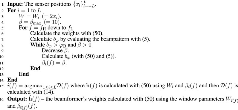
Algorithm 1. Algorithm for calculating the beamformer weights.

By choosing the window support to equal W = 2x_L (as done in (Long et al., 2019)), we are left with a single parameter to tune, β. We increase the degrees of freedom of the problem by optimizing over the parameter W. We consider multiple values of W (per frequency), and for each W, tune β so that the beamwidth is as desired. Then, per frequency, we select the W that achieves the highest DF. To reduce the number of possible values of W we limit the window support to the set ${\left\{W_i\right\}}_{i=1}^L$ of size L where W_i = 2x_i. Here, W_i corresponds to having only the 2i + 1 center sensors having nonzero weights. We refer to these sensors as active sensors. In the results, we show that the performance improvement of not limiting the values of W to this set is negligible. Therefore, we limit the values of W to this set to reduce the computational complexity of finding the weights. Notice that W is optimized per frequency, i.e., W = W(f).

To reflect that some sensors are closely spaced, we use the trapezoidal integration technique (TIT), i.e., we multiply each weight by ${\mathrm{\Delta }}_l=\frac{x_{l+1}-x_{l-1}}{2}$ as was done in (Ward et al., 2001). We multiply the weight of the outermost sensors by Δ_L = Δ_−L = x_L − x_L−1. Altogether,

${\mathrm{\Delta }}_l=\left\{\begin{array}{cc}\frac{x_{l+1}-x_{l-1}}{2}\hfill & ,\left|l\right|<L,\hfill \\ x_L-x_{L-1}\hfill & ,\left|l\right|=L.\hfill \end{array}\right.(49)$

By using the TIT at frequencies where all of the sensors are used (W = 2x_L), the center sensors that are close together have less influence. This enables maintaining the desired beamwidth at low frequencies.

Last, we normalize the weights to fulfill (4). To conclude, the beamformer weights are:

$h\left[l\right]=\frac{{\mathrm{\Delta }}_l{w}_{\text{K}}\left(x_l\right)}{\sum _{l^{\prime }=-L}^L{\mathrm{\Delta }}_{l^{\prime }}{w}_{\text{K}}\left(x_{l^{\prime }}\right)},-L\le l\le L.(50)$

After the weights are found for each frequency, the DI can be evaluated. Algorithm 1 summarizes the process. The resulting beamformer weights, $\widehat{\mathbf{h}}(f)$, satisfy the constraints in (45). So, we proceed with determining where to place the sensors.

Computational Complexity of Algorithm 1:

Calculating the weights with (50) requires M multiplications for computing the products ${\mathrm{\Delta }}_l{w}_{\text{K}}\left(x_l\right)$, − L ≤ l ≤ L. Because we begin with the largest β, the beamwidth is initially wider than desired, and thus the absolute value of the beampattern at azimuth $\phi ={\phi }_{\text{d}}+\frac{1}{2}{\phi }_{\text{B}}$ is greater than $1/\sqrt{2}$. Therefore, to check whether b_φ > φ_B, it is sufficient to evaluate the absolute value of the beampattern at azimuth $\phi ={\phi }_{\text{d}}+\frac{1}{2}{\phi }_{\text{B}}$ and check whether it is greater than $1/\sqrt{2}$, requiring M multiplications. Let B denote the number of window shape factor options. The beampattern is evaluated up to F + B times per window support option, thus evaluated for up to a total of $\left(F+B\right)L$ times. Altogether, the first part of the algorithm requires $\mathcal{O}\left(M^2\left(F+B\right)\right)$ computations.

In the second part of the algorithm, calculating the DF requires M multiplications for calculating the weights and M² + M multiplications for the matrix multiplications, per frequency and window support option. Therefore, requires $\mathcal{O}\left(M^{3}F\right)$ computations.

In total, Algorithm 1 requires $\mathcal{O}\left(M^2\left(MF+B\right)\right)$ computations.

4.2 Symmetric Linear Array Sensor Positioning

Our goal is to find where to position the sensors such that the DI is maximized while using the weight design proposed in the previous subsection. Formally,

$\underset{x_l,-L\le l\le L}{\mathrm{m}\mathrm{a}\mathrm{x}\mathrm{i}\mathrm{m}\mathrm{i}\mathrm{z}\mathrm{e}}{\mathcal{D}I}_{\left[f_{\text{L}},f_{\text{H}}\right]},(51)$

where the weights are attained using Algorithm 1; these weights fulfill the constraints in (45). A brute force search over all possible positions is infeasible. So, we first present an iterative algorithm for determining the sensor positions. The resulting performance is an upper bound on the DI (using the weight design proposed in the previous section). Afterward, we present a simpler algorithm that achieves competitive performance.

4.2.1 Iterative Algorithm

The sensor positions are iteratively updated to maximize the DI using the Nelder-Mead simplex algorithm (Lagarias et al., 1998). A set of L variables represent the sensor positions ${\left\{x_l\right\}}_{l=1}^L$. The ${\mathcal{D}I}_{\left[f_{\text{L}},f_{\text{H}}\right]}$ is evaluated in each iteration by constructing the symmetric array by (44), finding the beamformer’s weights according to Algorithm 1, and finally calculating the DI with (16). The algorithm is initialized multiple times with different starting points to ensure that a global maximum is found. Therefore, the resulting DI is an upper bound on the DI (using the weight design proposed in the previous section).

4.2.2 Non-Iterative Algorithm

In this section, we outline steps to achieve a constant beamwidth over a maximum range of frequencies. Afterward, we modify one of the steps to improve the DI at the expense of reducing the frequency range.

The algorithm is initialized with a symmetric linear array with M₀ = 2L₀ + 1 (<M) sensors. When these sensors are active, the lowest frequency that can maintain the desired beamwidth is attained using the widest window (β = 0). Denote this frequency by $f_{\text{min}}^{(L_0)}$. We add a pair of sensors with symmetric positions. Denote by $d^{(L_0+1)}$ the interelement spacing between the new sensor to the previously outermost sensor. It is desirable for $d^{(L_0+1)}$ to be large so that the array can support low frequencies. However, if it is too large, the beamwidth at higher frequencies (specifically, at $f_{\text{min}}^{(L_0)}$) is too narrow. So, $d^{(L_0+1)}$ is chosen such that above $f_{\text{min}}^{(L_0)}$ the new pair of sensors are inactive and below $f_{\text{min}}^{(L_0)}$ the new pair of sensors are active. Therefore, we increase $d^{(L_0+1)}$ so long as the array can maintain the desired beamwidth at $f_{\text{min}}^{(L_0)}$. Because $f_{\text{min}}^{(L_0)}$ is the highest frequency that the new sensors are active at, the desired beamwidth is attained there with the narrowest window: β = β_max (= 10). The process of adding a pair of sensors is repeated until the array consists of M sensors.

As displayed in the results, the sidelobes are high for low values of β: decreasing the DI. Therefore, we limit the widest window to β = β_min > 0. This modification improves the DI but reduces the frequency range because the beampattern cannot be as narrow as when β = 0. We need to initialize with M₀ = 5 sensors because three cannot attain a narrow enough beamwidth at f_H = 8 kHz without exhibiting high sidelobes. An option how to choose the initial M₀ sensors: a ULA with M₀ sensors whose interelement spacing is determined to maximize the DF at f_H. The steps are detailed in Algorithm 2.

ALGORITHM 2

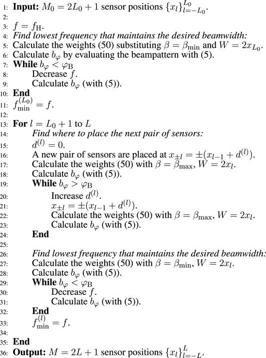
Algorithm 2. Algorithm for computing the optimal sensor positions.

The algorithm can be used to determine how many sensors are necessary to maintain a constant beamwidth over the frequency band [f_L, f_H]. Once f ≤ f_L, we can finish adding new pairs of sensors. Once the positions are found with Algorithm 2, the beamformer weights are obtained with Algorithm 1. Computational Complexity of Algorithm 2:

As detailed in the complexity analysis of Algorithm 1, $\mathcal{O}\left(M\right)$ operations suffice for checking whether b_φ > φ_B. Let D denote the number of position options. D is derived from the maximum permissible array aperture and the resolution in which d^(l) is increased in each iteration. The beampattern is evaluated up to D times in the part Find where to place the next pair of sensors, and up to F times in the part Find lowest frequency that maintains the desired beamwidth. Altogether, the beampattern is evaluated up to D + F times. Therefore, Algorithm 2 requires $\mathcal{O}\left(M\left(D+F\right)\right)$ computations.

5 Experimental Results

In this section, we examine the performance of our proposed approach and compare it to existing methods. We first examine linear arrays and compare our proposed iterative and non-iterative algorithms to existing methods. Next, we design planar arrays using the Kronecker and tradeoff beamformers.

5.1 Comparison of Linear Array With Previous Methods

In this section, we examine the performance of our proposed approach and compare it to previous approaches using M = 11 sensors. The desired half-power beamwidth is arbitrarily chosen to be φ_B = 15°. We compare our design method to three other methods: the sparse array design of Son (Son, 2021), the ULA design of Long et al. (Long et al., 2019), and the logarithmically spaced array design of Ward et al. (Ward et al., 2001). The array layouts are displayed in Figure 1.

FIGURE 1

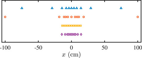
FIGURE 1. Configurations of the arrays: proposed (triangles), Son (circles), Long (squares), and Ward (diamonds).

Using the iterative algorithm proposed in the previous section, the resulting sensor positions of the symmetric linear array (for l ≥ 1) were [3.8, 7.9, 14.3, 29.2, 74.8] cm. To reproduce the array of Son (Son, 2021), we set the reference beampattern to equal

$\mathrm{s}\mathrm{i}\mathrm{n}\mathrm{c}\left(\frac{\phi -\frac{\pi }{2}}{0.2955}\right),(52)$

which has a half-power beamwidth of 15°. We also checked other reference beampatterns, yet they resulted in similar performances as using (52). An initial sensor with the highest spanning energy was chosen from a ULA with 2001 sensors and an interelement spacing of 0.1 cm. The remaining 2000 sensors were divided into five groups. From each group, two sensors closest to the group centroid were chosen. Finally, the sparse array was created with the 11 chosen sensors. Next, the weights were found. The mainlobe error tolerances were 0.006E₁ for φ ∈ [82.5°, 97.5°]. The sidelobe error tolerances were 0.028E₂ for φ ∈ [0°, 82.5°) ∪ (97.5°, 180°]. Here, E₁ = 31 and E₂ = 330 were the number of azimuth angles sampled (the resolution was 0.5°). To ensure that the beamwidth was as desired, we added two constraints: that the error tolerances were 0.0001 for φ ∈ {82.5°, 97.5°}. The resulting sparse array was a symmetric linear array with real weights. The ULA weights used by Long et al. (Long et al., 2019) were reproduced using Algorithm 1, where the window support was limited to only equal the support of the array, i.e., W ≡ 2x_L. For the comparison, we used an interelement spacing of 2.8 cm because it resulted in the largest ${\mathcal{D}I}_{\left[0,8\mathrm{k}\mathrm{H}\mathrm{z}\right]}$ while attaining a beamwidth of at least 15° at all frequencies. To reproduce the array of Ward et al. (Ward et al., 2001), we set the reference beampattern to equal (52). We used a logarithmic ratio of 3 (denoted by Q in (Ward et al., 2001)) because it resulted in the highest DI.

The optimal window parameters (β and W for our array and β for Long) were calculated using Algorithm 1 and are plotted in Figure 2 as a function of frequency. As expected, for frequencies with the same number of active sensors, β increases as the frequency increases. This is necessary to counteract the narrowing of the beampattern as the frequency increases. Increasing β narrows the Kaiser window, which in turn widens the beamwidth due to the inverse relationship between the window width and the beamformer width. We also observe that the number of active sensors (2i + 1) decreases as the frequency increases. Reducing the number of active sensors narrows the window, yielding an effect similar to increasing β.

FIGURE 2

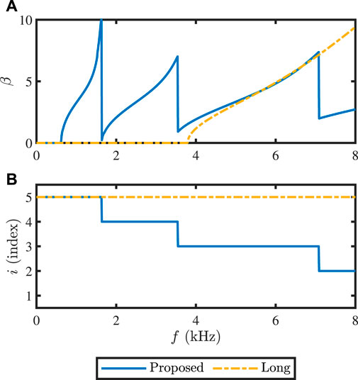
FIGURE 2. Continuous Kaiser window parameters, (A) the window shape factor, and (B) the index of the window support from the set ${\left\{2x_i\right\}}_{i=1}^5$, as a function of frequency: proposed (solid line) and Long (dashed line).

The beamformer weights (computed by (50) for our array and by (47) followed by normalization to fulfill (4) for Long) are illustrated in Figure 3. For the proposed and Ward arrays, the inner sensors are effectively inactive at low frequencies due to the TIT (the TIT does not affect ULAs due to their uniform interelement spacing). The outer sensors are given greater weight due to their greater distance between adjacent sensors (49). This enables maintaining the desired beamwidth at low frequencies by effectively widening the window. With these weights, the beampatterns were constructed according to (5) and are illustrated in Figure 3. The beamwidth, WNG, and DF are plotted in Figure 4 as a function of frequency. Son’s method performance is only reported at frequencies where the WNG is at least 0 dB (f ≥ 350 Hz). Our array maintained the desired beamwidth down to 620 Hz, while Long could not hold the desired beamwidth below 3.77 kHz. Ward’s array does not exhibit a constant beamwidth; Ward needed more sensors to succeed. Son’s array maintained the desired beamwidth down to 350 Hz but had lower WNG and DI than ours. Son’s and ours arrays’ WNG was lower than Long’s and Ward’s due to fewer active sensors at each frequency, as shown in Figure 3A.

FIGURE 3

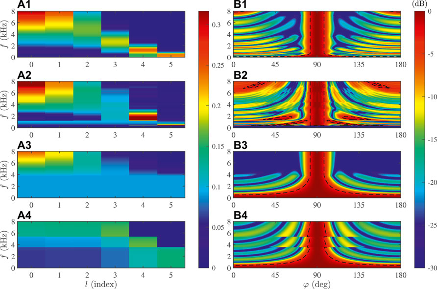
FIGURE 3. The left subplots (A) illustrate the weight values of the arrays: (1) proposed, (2) Son, (3) Long, and (4) Ward. For each array, the weights are given per sensor as a function of frequency. The right subplots (B) illustrate the beampatterns. The overlayed dashed line is the half-power contour of the mainlobe.

FIGURE 4

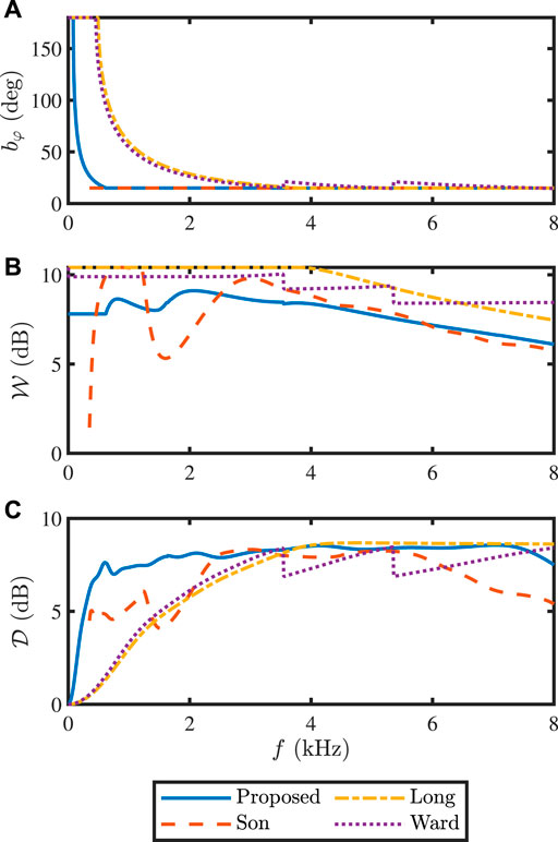
FIGURE 4. (A) Beamwidth, (B) WNG, and (C) narrowband directivity factor as a function of frequency: proposed (solid line), Son (dashed line), Long (dash-dot line), and Ward (dotted line). The obtained ${\mathcal{W}}_{\left[350\mathrm{H}\mathrm{z},8\mathrm{k}\mathrm{H}\mathrm{z}\right]}$ are respectively 7.8, 7.6, 9.5, and 9.2 dB. The obtained ${\mathcal{D}I}_{\left[350\mathrm{H}\mathrm{z},8\mathrm{k}\mathrm{H}\mathrm{z}\right]}$ are respectively 8.1, 6.7, 6.5, and 6.3 dB.

From the DF, the DI was calculated using (16). The ${\mathcal{D}I}_{\left[0,8\mathrm{k}\mathrm{H}\mathrm{z}\right]}$ of the proposed, Long, and Ward arrays are 7.6, 5.9, and 5.7 dB, respectively; the ${\mathcal{D}I}_{\left[350\mathrm{H}\mathrm{z},8\mathrm{k}\mathrm{H}\mathrm{z}\right]}$ of the proposed array is 1.4 dB better than Son’s. This demonstrates the advantage of our proposed design.

5.2 Beamformer Weights Design

In this section, we discuss the properties of the proposed weight design. We report the degradation in performance of the proposed configuration when one of the design steps is omitted.

The TIT improved the ${\mathcal{D}I}_{\left[0,8\mathrm{k}\mathrm{H}\mathrm{z}\right]}$ by 0.6 dB and enabled maintaining the desired beamwidth at lower frequencies (an extra 410 Hz), proving the technique’s added value. The TIT gives larger weight to the outer sensors because of their greater distance between adjacent sensors (49). This enables maintaining the desired beamwidth at low frequencies by effectively widening the window.

Sampling the continuous Kaiser window at the element positions according to (48) led to a modest improvement of 0.05 dB over uniformly sampling the window according to (47). The ${\mathcal{D}I}_{\left[0,8\mathrm{k}\mathrm{H}\mathrm{z}\right]}$ improvement when using continuous values of W without limiting W to the set ${\left\{2x_i\right\}}_{i=1}^L$ was negligible (0.01 dB), therefore, it is sufficient to limit the window support to this set. Although, if we were to limit the window support to only equal the support of the array, i.e., W ≡ 2x_L, the beamwidth would be narrower than 15° at frequencies above 1.63 kHz. This shows the merit of setting a subset of the sensors to be active to widen the beampattern at higher frequencies effectively.

Last, we examine the performance when we limited the array configuration to be an M = 11 sensor ULA. To find the ULA’s optimal configuration, the iterative algorithm proposed in the previous section optimized one variable that represented the interelement spacing. The resulting interelement spacing of the ULA was 4.1 cm and its ${\mathcal{D}I}_{\left[350\mathrm{H}\mathrm{z},8\mathrm{k}\mathrm{H}\mathrm{z}\right]}$ was 7.2 dB—still better than Son, Long, and Ward.

5.3 Non-iterative Algorithm’s Performance

Here we display the properties of our proposed non-iterative algorithm for determining the sensor positions. We compare the iterative and non-iterative algorithms. For the iterative algorithm, we used the same array design as in the previous section. For the non-iterative algorithm, we initialized with a ULA of M₀ = 5 sensors with an interelement spacing of 3.4 cm. We used this spacing because it maximized the DF at f_H = 8 kHz. We initialized with M₀ = 5 sensors because three cannot attain the desired beamwidth at 8 kHz without exhibiting high sidelobes. We set f_H = 8 kHz, M = 11, β_max = 10, and φ_B = 15°.

We constructed two arrays using the non-iterative algorithm (detailed in Algorithm 2). For one array, we set β_min = 0, and for the other array, we choose β_min = 1.36 so that the minimum frequency for the desired beamwidth is the same as that obtained with the iterative algorithm (620 Hz). The resulting sensor positions are displayed in Figure 5. After the positions were chosen, the optimal window parameters were found using Algorithm 1 and are plotted in Figure 6. The beamwidth, WNG, and DF are plotted in Figure 7 as a function of frequency.

FIGURE 5

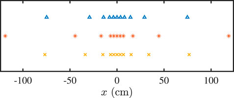
FIGURE 5. Configurations of the arrays: iterative (triangles), non-iterative with β_min = 0 (asterisks), and non-iterative with β_min = 1.36 (crosses).

FIGURE 6

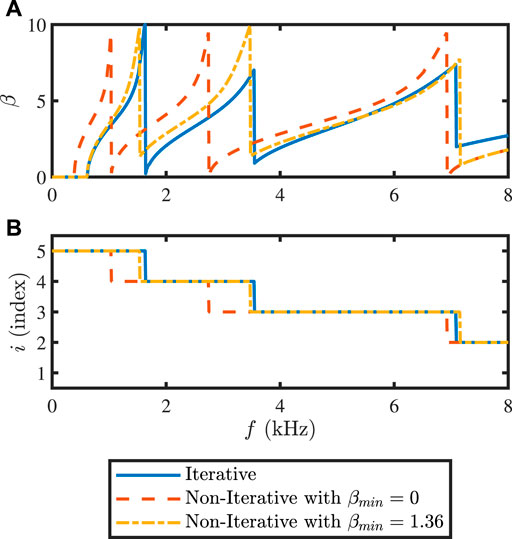
FIGURE 6. Continuous Kaiser window parameters, (A) the window shape factor, and (B) the index of the window support from the set ${\left\{2x_i\right\}}_{i=1}^5$, as a function of frequency: iterative (solid line), non-iterative with β_min =0 (dashed line), and non-iterative with β_min =1.36 (dash-dot line).

FIGURE 7

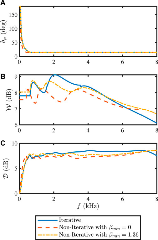
FIGURE 7. (A) Beamwidth, (B) WNG, and (C) narrowband directivity factor as a function of frequency: iterative (solid line), non-iterative with β_min = 0 (dashed line), and non-iterative with β_min = 1.36 (dash-dot line). The obtained ${\mathcal{W}}_{\left[0,8\mathrm{k}\mathrm{H}\mathrm{z}\right]}$ are respectively 7.8, 7.5, and 7.8 dB. The obtained ${\mathcal{D}I}_{\left[0,8\mathrm{k}\mathrm{H}\mathrm{z}\right]}$ are respectively 7.6, 7.3, and 7.4 dB.

For the array designed with β_min = 0, we see that as the frequency decreases, right before another sensor is activated, the window is as wide as possible (β = 0). For the array designed with β_min = 1.36, we see that the optimal window parameter, β, is sometimes less than 1.36. This is plausible because β_min was used only for choosing where to place the sensors. Afterward, Algorithm 1 may use any value of β.

We see that setting β_min > 0 resulted in improved directivity compared to β_min = 0. As expected, the iterative algorithm produced an array with a larger DI than the non-iterative algorithm. Nevertheless, the ${\mathcal{D}I}_{\left[0,8\mathrm{k}\mathrm{H}\mathrm{z}\right]}$ obtained with the non-iterative algorithm was only 0.2 dB smaller. This is beneficial considering the computational simplicity of the non-iterative algorithm compared to the iterative algorithm: no optimization toolbox is needed for the non-iterative algorithm.

5.4 Planar Array

This section compares our proposed techniques for constant-beamwidth beamforming for planar arrays to Son’s design (Son, 2021) using 99 sensors. The array layouts are displayed in Figure 8. The desired half-power beamwidths were arbitrarily chosen to be θ_X = 15° in the XZ plane and θ_Y = 30° in the YZ plane.

FIGURE 8

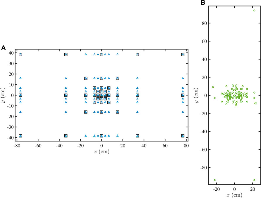
FIGURE 8. (A) Configurations of the arrays: proposed planar (triangles) and proposed star (squares). (B) Configuration of Son’s array (circles).

To construct the planar array, we first design two linear arrays. To find the positions of the sensors, we use the non-iterative algorithm proposed in the previous section: we design a symmetric linear array with M = 11 sensors with a constant beamwidth of θ_X = 15° and another symmetric linear array with N = 9 sensors with a constant beamwidth of θ_Y = 30°. We initialize with a ULA of M₀ = 5 sensors with an interelement spacing of 3.4 cm. For the first array, we set β_min = 1.36, and for the second array, we set β_min = 1.00 so that the minimum frequencies that the beampatterns still maintain the desired beamwidths are both 620 Hz. Fewer sensors are needed in the second array because the desired beamwidth is wider. We use the non-iterative algorithm instead of the iterative algorithm because of its low computational complexity while attaining on-par performance. The beamformer weights for the two symmetric linear arrays are computed using Algorithm 1.

Based on the linear arrays’ sensor positions, we construct a symmetric planar array with a total of MN = 99 sensors. For this proposed layout, four different beamformer weight vectors are compared. For Kronecker product beamforming, the weights are given by the Kronecker product of the linear arrays’ weights (27). The beamformer weights for maximum WNG, tradeoff, and maximum directivity are given by (43), where we set α ∈ {1, 0.5, 0.01}, respectively.

To reproduce the array of Son (Son, 2021), we set the reference beampattern to equal

$\mathrm{s}\mathrm{i}\mathrm{n}\mathrm{c}\left(\frac{\theta }{-0.1477\cos \left(2\phi \right)+0.4432}\right),(53)$

which has a half-power beamwidth of 15° in the XZ plane and 30° in the YZ plane. From a uniform planar array with 201 × 201 sensors and an interelement spacing of 1 cm, an initial 30 sensors with the highest spanning energy were chosen. The remaining sensors were divided into 23 groups. From each group, three sensors closest to the group centroid were chosen. Finally, the sparse array was created with the 99 chosen sensors. Next, the weights were found. The mainlobe error tolerances were 0.006E₁ for θ ∈ [0°, 15°]. The sidelobe error tolerances were 0.028E₂ for θ ∈ (15°, 90°]. Here, E₁ = 31 × 181 and E₂ = 150, ×, 181 were the number of angles sampled (the azimuth and elevation resolutions were 2° and 0.5°, respectively). To ensure that the beamwidths were as desired, we added four constraints: that the error tolerances were 0.0001 for (φ, θ) ∈ {(0°, 7.5°), (90°, 15°), (180°, 7.5°), (270°, 15°)}. The resulting sparse array was not symmetric and had complex-valued weights.

With these weights, the beampatterns were constructed according to (5) and illustrated for a few frequencies in Figure 9. The beamwidths in the XZ and YZ planes of the proposed and Son’s beamformers are plotted in Figure 10 as a function of frequency. The beamwidths of the proposed beamformers were the same as the beamwidths of the linear arrays upon which they were built. For the Kronecker beamformer, this is due to property (28), and for the other beamformers, this is due to the constraint (37). Therefore, the proposed techniques maintained the desired beamwidth down to 620 Hz. Son’s array maintained the desired beamwidths at even lower frequencies. We see in Figure 10 that Son’s beamwidth was narrower than desired at some frequencies. This was because the beampattern dipped below $1/\sqrt{2}$ and then peaked back to $1/\sqrt{2}$ at $\frac{1}{2}{\theta }_{\text{Y}}$ as constrained.

FIGURE 9

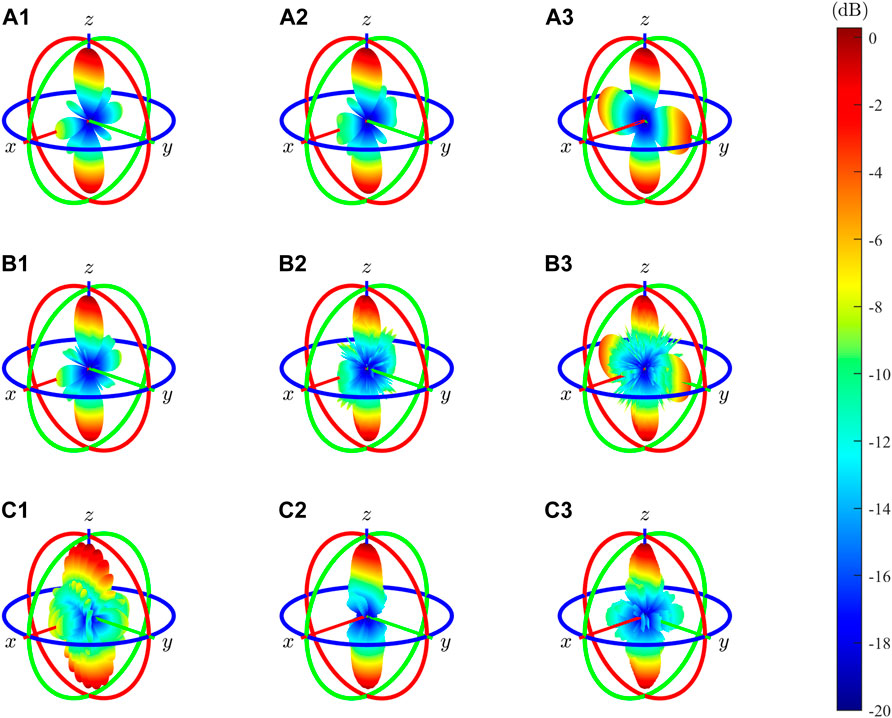
FIGURE 9. Planar arrrays’ beampatterns using the beamformers: (A) proposed Kronecker, (B) proposed tradeoff with α = 0.5, and (C) Son, for several frequencies: (1) 2 kHz, (2) 5 kHz, and (3) 8 kHz.

FIGURE 10

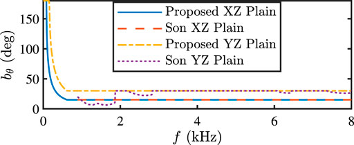
FIGURE 10. Beamwidths in the XZ and YZ planes as a function of frequency of Son’s and our proposed planar beamformers.

The WNG and DF are plotted in Figure 11 as a function of frequency. Son’s performance is only reported at frequencies where the WNG is at least 0 dB (f ≥ 890 Hz). For most frequencies, the WNGs of our design techniques were lower than Son’s. This was expected because Son’s objective was to maximize the WNG. We also see that the larger α was for the proposed techniques, the larger the WNG.

FIGURE 11

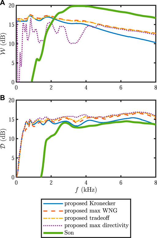
FIGURE 11. (A) WNG, and (B) narrowband directivity factor as a function of frequency: Kronecker (solid line), max WNG (dashed line), tradeoff (dash-dot line), max directivity (dotted line), and Son (thick solid line). The obtained ${\mathcal{W}}_{\left[890\mathrm{H}\mathrm{z},8\mathrm{k}\mathrm{H}\mathrm{z}\right]}$ are respectively 13.5, 15.0, 14.9, 13.0, and 13.1 dB. The obtained ${\mathcal{D}I}_{\left[890\mathrm{H}\mathrm{z},8\mathrm{k}\mathrm{H}\mathrm{z}\right]}$ are respectively 14.4, 15.2, 15.5, 15.8, and 6.1 dB.

From the DF, the DI was calculated using (16). The ${\mathcal{D}I}_{\left[890\mathrm{H}\mathrm{z},8\mathrm{k}\mathrm{H}\mathrm{z}\right]}$ of the proposed techniques were higher than achieved by Son. This demonstrates the advantage of the proposed techniques. We also see that the smaller α was for the proposed techniques, the larger the DI. It is important to note that the tradeoff beamformer has greater WNG and DI than the Kronecker beamformer. The Kronecker beamformer’s performance is inferior because it obtains the desired beamwidths without solving an optimization problem.

A major advantage of our technique over Son’s is the computational complexity. We report the running times on an Intel^ⓒ Core™ i7-8550U CPU with 8 GB RAM with the code implemented in MATLAB. For the tradeoff beamformer, it took 3 s to find the sensor positions for the two linear arrays using the non-iterative algorithm, 17 s to compute the weights with Algorithm 1 (the resolution of β was 0.01), and 33 s to calculate the beamformer weights (for all 801 frequencies). In total: less than 1 min. On the other hand, for Son, it took 279 s to choose the positions of the sensors and 286 s to calculate the beamformer weights for one frequency. To calculate for all 801 frequencies, Son’s technique took more than 1,000 times longer than ours.

Last, we examine the performance when limiting the array configuration to an 11 × 11 planar array with uniform spacing. We construct two ULAs (each with M = 11 sensors) with an interelement spacing of 4.2 cm to find the sensor positions. We use this spacing because it results in the highest ${\mathcal{D}I}_{\left[0,8\mathrm{k}\mathrm{H}\mathrm{z}\right]}$ while maintaining a beamwidth at least as wide as desired for all frequencies. We use Algorithm 1 to find the weights for both ULAs: for one the desired beamwidth was θ_X = 15° and for the other the desired beamwidth was θ_Y = 30°. From these two ULAs, we construct a planar array (with an interelement spacing of 4.2 cm) where the weights are given by the tradeoff beamformer (43) with α = 0.01 to maximize the directivity. Its ${\mathcal{D}I}_{\left[0,8\mathrm{k}\mathrm{H}\mathrm{z}\right]}$ was 11.2 dB—lower by at least 1.3 dB than our proposed nonuniformly spaced planar array beamformers, even though it had 121 sensors. This is similar to what we have seen for the linear arrays: the nonuniformly spaced array achieves greater DI.

5.5 Planar Array With Missing Sensors

In this section, we simulate a planar array with sensors only at some of the grid positions. We use the same planar array design from the previous section. However, we place sensors at only S = 39 out of the MN = 99 grid positions. In addition, we choose to place the sensors in a way that resembles a star. The selected grid positions are displayed in Figure 8 and called the star array. Because only a subset of the grid positions is used, the Kronecker product beamformer is invalid here. Therefore, we only compare three different beamformers: the beamformers given by (43) with α ∈ {1, 0.5, 0.01}, for maximum WNG, tradeoff, and maximum directivity, respectively. With the beamformers’ weights, the beampatterns were constructed according to (5) and are illustrated for a few frequencies in Figure 12. The beamwidths are shown in Figure 10. Even though we only placed sensors at a subset of the grid positions, the beamformers still maintain the desired beamwidth down to 620 Hz. The WNG and DF are plotted in Figure 13 as a function of frequency. As expected, the larger is α, the higher is the WNG and the lower is the DI. The ${\mathcal{D}I}_{\left[890\mathrm{H}\mathrm{z},8\mathrm{k}\mathrm{H}\mathrm{z}\right]}$ of the S = 39 sensor star array is still higher than achieved by Son’s sparse 99 sensor array. This demonstrates the advantage of the proposed technique.

FIGURE 12

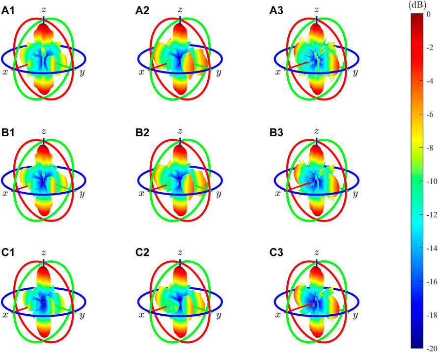
FIGURE 12. Star array’s beampatterns using the beamformers: (A) max WNG, (B) tradeoff, and (C) max directivity, for several frequencies: (1) 2 kHz, (2) 5 kHz, and (3) 8 kHz.

FIGURE 13

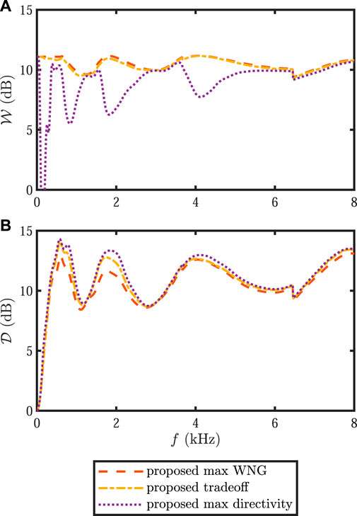
FIGURE 13. (A) WNG, and (B) narrowband directivity factor as a function of frequency for the star array beamformers: max WNG (dashed line), tradeoff (dash-dot line), and max directivity (dotted line). The obtained ${\mathcal{W}}_{\left[890\mathrm{H}\mathrm{z},8\mathrm{k}\mathrm{H}\mathrm{z}\right]}$ are respectively 10.4, 10.3, and 9.2 dB. The obtained ${\mathcal{D}I}_{\left[890\mathrm{H}\mathrm{z},8\mathrm{k}\mathrm{H}\mathrm{z}\right]}$ are respectively 10.5, 10.8, and 11.0 dB.

We compare the performance of the star array to a 7 × 7 planar array with uniform spacing. To find the positions of the sensors, we construct two ULAs (each with M = 7 sensors) with an interelement spacing of 4.3 cm. We use this spacing because it results in the highest ${\mathcal{D}I}_{\left[0,8\mathrm{k}\mathrm{H}\mathrm{z}\right]}$ while maintaining beamwidths that are at least as wide as desired for all frequencies. We use Algorithm 1 to find the weights for both ULAs: for one the desired beamwidth is θ_X = 15°, and for the other the desired beamwidth is θ_Y = 30°. From these two ULAs, we construct a uniform planar array (with an interelement spacing of 4.3 cm) where the weights are given by the tradeoff beamformer (43) with α = 0.01 to maximize the directivity. Its ${\mathcal{D}I}_{\left[0,8\mathrm{k}\mathrm{H}\mathrm{z}\right]}$ is 8.7 dB—lower by at least 0.4 dB than our nonuniformly spaced star array beamformers, even though it has 49 sensors. This once again shows the value of using a nonuniformly spaced design.

6 Conclusion

We have proposed planar beamformers that yield different beamwidths in the XZ and YZ planes by designing constant-beamwidth linear arrays. The planar beamwidths equal the linear array beamwidths for all frequencies. The first technique involves utilizing Kronecker product properties, whereby no matrix inversion is needed to find the weights. Our second technique provides a closed-form solution that allows a tradeoff between WNG and directivity. The second technique is applicable even when only a subset of the sensors is used. Further research is needed to choose the optimal subset of the sensors.

As a building block for the planar beamformer, we proposed a method to find optimal sensors placements in a symmetric nonuniform linear array and optimal beamformer to maximize the DI. The design involves sampling the continuous Kaiser window, varying the window support, and using the TIT. Sampling the continuous Kaiser window at the sensor positions is appropriate given the nonuniform interelement spacing of the symmetric array. Varying the window support and the window shape factor enables more control over the effective width of the window. Using the TIT allows for maintaining the desired beamwidth at low frequencies. Experimental results have shown that the proposed techniques yield higher directivity and involve lower computational complexity than the state-of-the-art. Additionally, the resulting symmetric nonuniform arrays outperform uniformly-spaced arrays. Future work will focus on generalizing the proposed methods to three-dimensional arrays and addressing the problem of constant-beamwidth steering with nonuniform arrays.

Data Availability Statement

The original contributions presented in the study are included in the article/Supplementary Material, further inquiries can be directed to the corresponding authors.

Author Contributions

AF contributed to methodology, investigation, formal analysis, software, validation, and writing—original draft. IC contributed to conceptualization, methodology, supervision, and writing—review and editing.

Funding

This work was supported by the Pazy Research Foundation.

Conflict of Interest

The authors declare that the research was conducted in the absence of any commercial or financial relationships that could be construed as a potential conflict of interest.

Publisher’s Note

All claims expressed in this article are solely those of the authors and do not necessarily represent those of their affiliated organizations, or those of the publisher, the editors and the reviewers. Any product that may be evaluated in this article, or claim that may be made by its manufacturer, is not guaranteed or endorsed by the publisher.

Acknowledgments

The authors would like to thank Stem Audio for providing equipment and technical guidance.

References

Aroudi, A., and Braun, S. (2021). “Dbnet: Doa-Driven Beamforming Network for End-To-End Reverberant Sound Source Separation,” in ICASSP 2021-2021 IEEE International Conference on Acoustics, Speech and Signal Processing (ICASSP (IEEE), 211–215. doi:10.1109/icassp39728.2021.9414187

CrossRef Full Text | Google Scholar

Benesty, J., Cohen, I., and Chen, J. (2019). Array Processing: Kronecker Product Beamforming, 18. Springer.

Google Scholar

Benesty, J., Cohen, I., and Chen, J. (2018). Fundamentals of Signal Enhancement and Array Signal Processing. Wiley Online Library.

Google Scholar

Buchris, Y., Amar, A., Benesty, J., and Cohen, I. (2018). Incoherent Synthesis of Sparse Arrays for Frequency-Invariant Beamforming. IEEE/ACM Trans. Audio, Speech, Lang. Process. 27, 482–495.

Google Scholar

Buchris, Y., Cohen, I., Benesty, J., and Amar, A. (2020). Joint Sparse Concentric Array Design for Frequency and Rotationally Invariant Beampattern. Ieee/acm Trans. Audio Speech Lang. Process. 28, 1143–1158. doi:10.1109/taslp.2020.2982287

CrossRef Full Text | Google Scholar

Chan, S., and Chen, H. (2006). Uniform Concentric Circular Arrays with Frequency-Invariant Characteristics—Theory, Design, Adaptive Beamforming and Doa Estimation. IEEE Trans. Signal Process. 55, 165–177.

Google Scholar

Cohen, I., Benesty, J., and Chen, J. (2019). Differential Kronecker Product Beamforming. Ieee/acm Trans. Audio Speech Lang. Process. 27, 892–902. doi:10.1109/taslp.2019.2895241

CrossRef Full Text | Google Scholar

Cohen, I., Benesty, J., and Gannot, S. (2009). Speech Processing in Modern Communication: Challenges and Perspectives, 3. Springer Science & Business Media.

Google Scholar

Crocco, M., and Trucco, A. (2011). Design of Robust Superdirective Arrays with a Tunable Tradeoff between Directivity and Frequency-Invariance. IEEE Trans. Signal. Process. 59, 2169–2181. doi:10.1109/tsp.2011.2106780

CrossRef Full Text | Google Scholar

Erokhin, A., Gafarov, E., and Salomatov, Y. (2020). Frequency-invariant Beam Steering Based on Fir-Filters. Radioelectron.Commun.Syst. 63, 521–531. doi:10.3103/s0735272720100027

CrossRef Full Text | Google Scholar

Gazor, S., and Grenier, Y. (1995). Criteria for Positioning of Sensors for a Microphone Array. IEEE Trans. Speech Audio Process. 3, 294–303.

Google Scholar

Haupt, R. L., and Moosbrugger, P. (2012). “Maintaining a Constant Beamwidth when Scanning a Phased Array,” in 2012 IEEE International Conference on Wireless Information Technology and Systems (ICWITS) (IEEE), 1–4. doi:10.1109/icwits.2012.6417765

CrossRef Full Text | Google Scholar

Huang, G., Benesty, J., Chen, J., and Cohen, I. (2020a). “Robust and Steerable Kronecker Product Differential Beamforming with Rectangular Microphone Arrays,” in ICASSP 2020-2020 IEEE International Conference on Acoustics, Speech and Signal Processing (ICASSP) (IEEE), 211–215. doi:10.1109/icassp40776.2020.9052988

CrossRef Full Text | Google Scholar

Huang, G., Benesty, J., Cohen, I., and Chen, J. (2020b). A Simple Theory and New Method of Differential Beamforming with Uniform Linear Microphone Arrays. Ieee/acm Trans. Audio Speech Lang. Process. 28, 1079–1093. doi:10.1109/taslp.2020.2980989

CrossRef Full Text | Google Scholar

Huang, G., Cohen, I., Benesty, J., and Chen, J. (2020c). “Kronecker Product Beamforming with Multiple Differential Microphone Arrays,” in 2020 IEEE 11th Sensor Array and Multichannel Signal Processing Workshop (SAM) (IEEE), 1–5. doi:10.1109/sam48682.2020.9104333

CrossRef Full Text | Google Scholar

Itzhak, G., Benesty, J., and Cohen, I. (2019). Nonlinear Kronecker Product Filtering for Multichannel Noise Reduction. Speech Commun. 114, 49–59. doi:10.1016/j.specom.2019.10.001

CrossRef Full Text | Google Scholar

Itzhak, G., Benesty, J., and Cohen, I. (2021). On the Design of Differential Kronecker Product Beamformers. Ieee/acm Trans. Audio Speech Lang. Process. 29, 1397–1410. doi:10.1109/taslp.2021.3069089

CrossRef Full Text | Google Scholar

Kaiser, J., and Schafer, R. (1980). On the Use of the I₀-sinh Window for Spectrum Analysis. IEEE Trans. Acoust. Speech, Signal. Process. 28, 105–107. doi:10.1109/tassp.1980.1163349

CrossRef Full Text | Google Scholar

Kleiman, A., Cohen, I., and Berdugo, B. (2021). Constant-beamwidth Beamforming with Concentric Ring Arrays. Sensors 21, 7253. doi:10.3390/s21217253

PubMed Abstract | CrossRef Full Text | Google Scholar

Kuhn, E. V., Pitz, C. A., Matsuo, M. V., Bakri, K. J., Seara, R., and Benesty, J. (2021). A Kronecker Product Clms Algorithm for Adaptive Beamforming. Digital Signal. Process. 111, 102968. doi:10.1016/j.dsp.2021.102968

CrossRef Full Text | Google Scholar

Lagarias, J. C., Reeds, J. A., Wright, M. H., and Wright, P. E. (1998). Convergence Properties of the Nelder-Mead Simplex Method in Low Dimensions. SIAM J. Optim. 9, 112–147. doi:10.1137/s1052623496303470

CrossRef Full Text | Google Scholar

Li, S., Yang, X., Ning, L., Long, T., and Sarkar, T. K. (2017). “Broadband Constant Beamwidth Beamforming for Suppressing Mainlobe and Sidelobe Interferences,” in 2017 IEEE Radar Conference (RadarConf) (IEEE), 1041–1045. doi:10.1109/radar.2017.7944358

CrossRef Full Text | Google Scholar

Liu, R., Cui, G., Lu, Q., Yu, X., Feng, L., and Zhu, J. (2021). “Constant Beamwidth Receiving Beamforming Based on Template Matching,” in 2021 IEEE Radar Conference (RadarConf21) (IEEE), 1–5. doi:10.1109/radarconf2147009.2021.9455192

CrossRef Full Text | Google Scholar

Liu, W., and Weiss, S. (2008). Design of Frequency Invariant Beamformers for Broadband Arrays. IEEE Trans. Signal. Process. 56, 855–860. doi:10.1109/tsp.2007.907872

CrossRef Full Text | Google Scholar

Liu, W., Weiss, S., McWhirter, J. G., and Proudler, I. K. (2007). Frequency Invariant Beamforming for Two-Dimensional and Three-Dimensional Arrays. Signal. Process. 87, 2535–2543. doi:10.1016/j.sigpro.2007.03.018

CrossRef Full Text | Google Scholar

Liu, W., and Weiss, S. (2004). “New Class of Broadband Arrays with Frequency Invariant Beam Patterns,” in 2004 IEEE International Conference on Acoustics, Speech, and Signal Processing (IEEE). ii–185.2

Google Scholar

Liu, W., and Weiss, S. (2010). Wideband Beamforming: Concepts and Techniques, 17. John Wiley & Sons.

Google Scholar

Liu, Y., Cheng, J., Xu, K. D., Yang, S., Liu, Q. H., and Guo, Y. J. (2018). Reducing the Number of Elements in the Synthesis of a Broadband Linear Array with Multiple Simultaneous Frequency-Invariant Beam Patterns. IEEE Trans. Antennas Propagat. 66, 5838–5848. doi:10.1109/tap.2018.2862361

CrossRef Full Text | Google Scholar

Liu, Y., Zhang, L., Zhu, C., and Liu, Q. H. (2015). Synthesis of Nonuniformly Spaced Linear Arrays with Frequency-Invariant Patterns by the Generalized Matrix Pencil Methods. IEEE Trans. Antennas Propagat. 63, 1614–1625. doi:10.1109/tap.2015.2394497

CrossRef Full Text | Google Scholar

Long, T., Cohen, I., Berdugo, B., Yang, Y., and Chen, J. (2019). Window-based Constant Beamwidth Beamformer. Sensors 19, 2091. doi:10.3390/s19092091

PubMed Abstract | CrossRef Full Text | Google Scholar

Pal, P., and Vaidyanathan, P. (2010). “Efficient Frequency Invariant Beamforming Using Virtual Arrays,” in 2010 Conference Record of the Forty Fourth Asilomar Conference on Signals, Systems and Computers (IEEE), 1097–1101. doi:10.1109/acssc.2010.5757573

CrossRef Full Text | Google Scholar

Parra, L. C. (2006). Steerable Frequency-Invariant Beamforming for Arbitrary Arrays. The J. Acoust. Soc. America 119, 3839–3847. doi:10.1121/1.2197606

CrossRef Full Text | Google Scholar

Ramezanpour, P., Aghababaie, M., Mosavi, M., and M de Andrés, D. (2022). Multi-stage Beamforming Using Dnns. Iranian J. Electr. Electron. Eng., 2266.

Google Scholar

Rosen, O., Cohen, I., and Malah, D. (2017). Fir-based Symmetrical Acoustic Beamformer with a Constant Beamwidth. Signal. Process. 130, 365–376. doi:10.1016/j.sigpro.2016.07.019

CrossRef Full Text | Google Scholar

Sharma, R., Cohen, I., and Benesty, J. (2020). Adaptive and Hybrid Kronecker Product Beamforming for Far-Field Speech Signals. Speech Commun. 120, 42–52. doi:10.1016/j.specom.2020.04.001

CrossRef Full Text | Google Scholar

Sharma, R., Cohen, I., and Berdugo, B. (2021a). Controlling Elevation and Azimuth Beamwidths with Concentric Circular Microphone Arrays. Ieee/acm Trans. Audio Speech Lang. Process. 29, 1491–1502. doi:10.1109/taslp.2021.3072275

CrossRef Full Text | Google Scholar

Sharma, R., Cohen, I., and Berdugo, B. (2021b). “Window Beamformer for Sparse Concentric Circular Array,” in ICASSP 2021-2021 IEEE International Conference on Acoustics, Speech and Signal Processing (ICASSP) (IEEE), 4500–4504. doi:10.1109/icassp39728.2021.9414069

CrossRef Full Text | Google Scholar

Snow, W. B. (1931). Audible Frequency Ranges of Music, Speech and Noise. Bell Syst. Tech. J. 10, 616–627. doi:10.1002/j.1538-7305.1931.tb02334.x

CrossRef Full Text | Google Scholar

Son, P. L. (2021). On the Design of Sparse Arrays with Frequency-Invariant Beam Pattern. Ieee/acm Trans. Audio Speech Lang. Process. 29, 226–238. doi:10.1109/taslp.2020.3040033

CrossRef Full Text | Google Scholar

Tourbabin, V., Agmon, M., Rafaely, B., and Tabrikian, J. (2012). Optimal Real-Weighted Beamforming with Application to Linear and Spherical Arrays. IEEE Trans. Audio Speech Lang. Process. 20, 2575–2585. doi:10.1109/tasl.2012.2208626

CrossRef Full Text | Google Scholar

Van Trees, H. L. (2004). Optimum Array Processing: Part IV of Detection, Estimation, and Modulation Theory. John Wiley & Sons.

Google Scholar

Van Veen, B. D., and Buckley, K. M. (1988). Beamforming: A Versatile Approach to Spatial Filtering. IEEE ASSP Mag. 5, 4–24. doi:10.1109/53.665

CrossRef Full Text | Google Scholar

Wang, X., Benesty, J., Chen, J., Huang, G., and Cohen, I. (2021). Beamforming with Cube Microphone Arrays via Kronecker Product Decompositions. Ieee/acm Trans. Audio Speech Lang. Process. 29, 1774–1784. doi:10.1109/taslp.2021.3079816

CrossRef Full Text | Google Scholar

Wang, X., Benesty, J., Huang, G., Chen, J., and Cohen, I. (2019). Design of Kronecker product beamformers with cuboid microphone arrays (Universitätsbibliothek der RWTH Aachen).

Google Scholar

Wang, X., Huang, G., Benesty, J., Chen, J., and Cohen, I. (2020). Time Difference of Arrival Estimation Based on a Kronecker Product Decomposition. IEEE Signal. Process. Lett. 28, 51–55.

Google Scholar

Ward, D. B., Ding, Z., and Kennedy, R. A. (1998). Broadband Doa Estimation Using Frequency Invariant Beamforming. IEEE Trans. Signal. Process. 46, 1463–1469. doi:10.1109/78.668812

CrossRef Full Text | Google Scholar

Ward, D. B., Kennedy, R. A., and Williamson, R. C. (2001). “Constant Directivity Beamforming,” in Microphone Arrays (Springer), 3–17. doi:10.1007/978-3-662-04619-7_1

CrossRef Full Text | Google Scholar

Ward, D. B., Kennedy, R. A., and Williamson, R. C. (1995). Theory and Design of Broadband Sensor Arrays with Frequency Invariant Far‐field Beam Patterns. J. Acoust. Soc. America 97, 1023–1034. doi:10.1121/1.412215

CrossRef Full Text | Google Scholar

Weiss, S., Hadley, M., and Wilcox, J. (2017). “Implementation of a Flexible Frequency-Invariant Broadband Beamformer Based on Fourier Properties,” in 2017 Sensor Signal Processing for Defence Conference (SSPD) (IEEE), 1–5. doi:10.1109/sspd.2017.8233239

CrossRef Full Text | Google Scholar

Yan, S., and Ma, Y. (2005). “Design of Fir Beamformer with Frequency Invariant Patterns via Jointly Optimizing Spatial and Frequency Responses,” in Proceedings.(ICASSP’05). IEEE International Conference on Acoustics, Speech, and Signal Processing, 2005 (IEEE). 4. iv–789.

Google Scholar

Yan, S. (2006). Optimal Design of Fir Beamformer with Frequency Invariant Patterns. Appl. Acoust. 67, 511–528. doi:10.1016/j.apacoust.2005.09.008

CrossRef Full Text | Google Scholar

Yan, S., Sun, H., Ma, X., Svensson, U. P., and Hou, C. (2010). Time-domain Implementation of Broadband Beamformer in Spherical Harmonics Domain. IEEE Trans. audio, speech, Lang. Process. 19, 1221–1230.

Google Scholar

Yang, W., Huang, G., Benesty, J., Cohen, I., and Chen, J. (2019a). “On the Design of Flexible Kronecker Product Beamformers with Linear Microphone Arrays,” in ICASSP 2019-2019 IEEE International Conference on Acoustics, Speech and Signal Processing (ICASSP) (IEEE), 441–445. doi:10.1109/icassp.2019.8683768

CrossRef Full Text | Google Scholar

Yang, W., Huang, G., Chen, J., Benesty, J., Cohen, I., and Kellermann, W. (2020). Robust Dereverberation with Kronecker Product Based Multichannel Linear Prediction. IEEE Signal. Process. Lett. 28, 101–105.

Google Scholar

Yang, X., Li, S., Sun, Y., Long, T., and Sarkar, T. K. (2019b). Robust Wideband Adaptive Beamforming with Null Broadening and Constant Beamwidth. IEEE Trans. Antennas Propagat. 67, 5380–5389. doi:10.1109/tap.2019.2916607

CrossRef Full Text | Google Scholar

Yin, J.-x. (2012). “Directional Constant Beamwidth Beamforming by Second Order Cone Programming Constraints,” in In 2012 5th International Conference on BioMedical Engineering and Informatics (IEEE), 1443–1445. doi:10.1109/bmei.2012.6513112

CrossRef Full Text | Google Scholar

Zhao, Y., Liu, W., and Langley, R. (2009). “A Least Squares Approach to the Design of Frequency Invariant Beamformers,” in 2009 17th European Signal Processing Conference (IEEE), 844–848.

Google Scholar

Zhao, Y., Liu, W., and Langley, R. J. (2008). “Efficient Design of Frequency Invariant Beamformers with Sensor Delay-Lines,” in 2008 5th IEEE Sensor Array and Multichannel Signal Processing Workshop (IEEE), 335–339. doi:10.1109/sam.2008.4606884

CrossRef Full Text | Google Scholar

Zhao, Y., and Liu, W. (2012). Robust Fixed Frequency Invariant Beamformer Design Subject to Norm-Bounded Errors. IEEE Signal. Process. Lett. 20, 169–172.

Google Scholar

Zhu, W., and Wu, W. (2011). “Design of Wide-Band Array with Frequency Invariant Beam Pattern by Using Adaptive Synthesis Method,” in 2011 International Conference on Image Analysis and Signal Processing (IEEE), 688–693. doi:10.1109/iasp.2011.6109136

CrossRef Full Text | Google Scholar

Footnotes

¹https://github.com/Ariel12321/Constant_Beamwidth_Beamforming_Nonuniform