
94% of researchers rate our articles as excellent or good
Learn more about the work of our research integrity team to safeguard the quality of each article we publish.
Find out more
ORIGINAL RESEARCH article
Front. Soft Matter, 21 May 2024
Sec. Liquid Crystals
Volume 4 - 2024 | https://doi.org/10.3389/frsfm.2024.1359128
This article is part of the Research Topic1st Galapagos Soft Matter Conference - Research TopicView all 11 articles
 David Uriel Zamora Cisneros1
 Ziheng Wang1
 Noémie-Manuelle Dorval Courchesne1
 Matthew J. Harrington2
 Alejandro D. Rey1*
Background: Liquid crystal (LC) mesophases have an orientational and positional order that can be found in both synthetic and biological materials. These orders are maintained until some parameter, mainly the temperature or concentration, is changed, inducing a phase transition. Among these transitions, a special sequence of mesophases has been observed, in which priority is given to the direct smectic liquid crystal transition. The description of these transitions is carried out using the Landau–de Gennes (LdG) model, which correlates the free energy of the system with the orientational and positional order.
Methodology: This work explored the direct isotropic-to-smectic A transition studying the free energy landscape constructed with the LdG model and its relation to three curve families: (I) level-set curves, steepest descent, and critical points; (II) lines of curvature (LOC) and geodesics, which are directly connected to the principal curvatures; and (III) the Casorati curvature and shape coefficient that describe the local surface geometries resemblance (sphere, cylinder, and saddle).
Results: The experimental data on 12-cyanobiphenyl were used to study the three curve families. The presence of unstable nematic and metastable plastic crystal information was found to add information to the already developed smectic A phase diagram. The lines of curvature and geodesics were calculated and laid out on the energy landscape, which highlighted the energetic pathways connecting critical points. The Casorati curvature and shape coefficient were computed, and in addition to the previous family, they framed a geometric region that describes the phase transition zone.
Conclusion and significance: A direct link between the energy landscape’s topological geometry, phase transitions, and relevant critical points was established. The shape coefficient delineates a stability zone in which the phase transition develops. The methodology significantly reduces the impact of unknown parametric data. Symmetry breaking with two order parameters (OPs) may lead to novel phase transformation kinetics and droplets with partially ordered surface structures.
Synthetic and biological liquid crystals (LCs) are anisotropic soft materials with partial degrees of orientational and positional order, conveying fluidity as viscous liquids and anisotropy as in the crystalline order (Rey and Denn, 2002; Donald et al., 2006; Rey, 2010; Sonnet and Virga, 2012; Petrov, 2013; Lagerwall, 2016; Selinger, 2016; Collings and Goodby, 2019; Stewart, 2019; Zannoni, 2022). Importantly, possible LC mesogens include rod-, board-, disk-, and screw-like molecules with flexibilities ranging from semi-flexible to rigid, involving monomers or main/side-chain polymers and colloids (Donald et al., 2006; Demus et al., 2008b; Demus et al., 2011). The synthesis and formation of these mesophase materials follow equilibrium self-assembly processes driven by temperature (thermotropic), concentration (lyotropic), or both (Bowick et al., 2017; Wang et al., 2023b). The presence of multiple components, as in nanoparticle-loaded mesophases, gives rise to couplings between self-assembly and phase separation with states that can combine the crystallinity (positional order) of one component with the liquid crystallinity (various degrees of positional and orientational order) of the other (Soulé et al., 2012a; Soulé et al., 2012b; Soulé et al., 2012c; Soule and Rey, 2012; Milette et al., 2013; Gurevich et al., 2014). Various external fields (flow, electromagnetic, and thermal) can be used to generate self-organized structures not seen in purely equilibrium self-assembly. The natural setting to describe self-assembly starts with the energy landscape and its geometrical properties (curvatures, cusps, domes, etc.), while for non-equilibrium organization, the natural setting will include the entropy production landscape and its defining geometric measures. In this paper, we present a widely applicable geometry-based methodology for describing self-assembly in anisotropic soft matter and target one specific transition that exhibits complex ordering processes. Without ambiguity, for convenience and brevity, below we refer to self-assembly as phase ordering and/or phase transition, as we do not include phase separation and conserved quantities. In addition, we refer to the degree of quench as the equivalent of the thermodynamic driving force for phase ordering.
The spectrum of self-assembly processes is significantly enriched when considering the sequence of phase transformations. This progression follows an increase in order as the magnitude of the thermodynamic driving force is increased, corresponding to a decrease in temperature for thermotropes or an increase in concentration for lyotropes. The sequence then goes from a high-symmetry isotropic state to an orientationally ordered (nematic) state. This state is then followed by the addition of the positional order (smectic). Then, the crystalline organization is reached with a further increase in the driving force. The usual sequence of isotropic–orientational–positional phase ordering (Oswald and Pieranski, 2005a; Jákli and Saupe, 2006; Blinov, 2011) is sometimes reordered to a direct isotropic–positional/orientational ordering, as observed in monomeric thermotropes (certain cyano-biphenyls (CB) and oxy-cyanobiphenyls (OCB)) (Oh, 1977; Idziak et al., 1996; Oswald and Pieranski, 2005b; Donald et al., 2006; Abukhdeir and Rey, 2008; Chahine et al., 2010; Gudimalla et al., 2021; Nesrullajev, 2022) and biological liquid crystals (BLCs) such as collagen mesophase precursors in the mussel byssus (Knight and Vollrath, 1999; Viney, 2004; Donald et al., 2006; Rey, 2010; Rey and Herrera-Valencia, 2012; Rey et al., 2013; Renner-Rao et al., 2019; Manolakis and Azhar, 2020; Harrington and Fratzl, 2021; Berent et al., 2022). This important and non-classical behavior is the focus of this paper: the direct isotropic-to-smectic A (I-SmA) LC phase transition, where SmA denotes the simplest smectic phase. A collection of compounds exhibiting this scheme can be found (Hawkins and April 1983; Idziak et al., 1996; Lenoble et al., 2007; Abukhdeir and Rey, 2008; Mohieddin Abukhdeir and Rey, 2008a; Li et al., 2009; Wojcik et al., 2009; Chahine et al., 2010; Pouget et al., 2011; Salamonczyk et al., 2016; Bradley, 2019; Renner-Rao et al., 2019; Gudimalla et al., 2021; Jackson et al., 2021; Jehle et al., 2021; Khadem and Rey, 2021; Nesrullajev, 2022), which is largely driven by attractive forces in thermotropic LCs [e.g., cyanobiphenyl family (n-CB, n > 10) (Bellini et al., 2002)] and excluded volume interactions in BLCs (e.g., collagen in mussel byssus and Ff phages). In both cases, a common geometric feature is the presence of rigid or semi-rigid rod-like cores and sufficiently long semi-flexible ends. Currently, the best-characterized materials that follow the direct I-SmA are low-molar mass thermotropic LCs, such as 10CB and 12CB (Collings, 1997; Urban et al., 2005; Demus et al., 2008a; Li et al., 2009; Chahine et al., 2010; Gudimalla et al., 2021; Zaluzhnyy et al., 2022). To avoid introducing a plethora of unknown parameters and material data, we focus on them as model systems. In the future, our ultimate goal is to expand the findings to lyotropic polymeric and colloidal smectics that are found in collagen precursors of the mussel byssus (Renner-Rao et al., 2019; Jehle et al., 2021; Waite and Harrington, 2022). It is noted that even though we only consider thermotropic LCs in the current manuscript, using correspondence principles such as those provided in the following references (Picken, 1990; Soule and Rey, 2011; Golmohammadi and Rey, 2009; Doi, 1981), we can, in the future, use the current findings for collagen-based LCs.
A key feature of the I-SmA transition is the strong coupling of the positional and orientational order parameters (OPs) (Pikin, 1991; Gorkunov et al., 2007; Blinov, 2011; Turek et al., 2020; Gurin et al., 2021), which results in the enhancement of the orientational OP over and above what a nematic phase could show at these conditions of temperature or concentration. A practical consequence of this, as we know from synthetic liquid crystal polymers (LCPs), is that in the solid state, the enhanced orientational order parameter has a strong impact on the mechanical properties (e.g., Young modulus) that can be seen in LCP fibers (Ward, 1993; Ziabicki, 1993; Donald et al., 2006; Turek et al., 2020; Bunsell et al., 2021). This order parameter coupling decreases the free energy of the system to result in a smectic A phase at minimal quenches from the stable disordered state. Polymeric and biological liquid-crystalline materials, being part of the lyo/thermotropic spectrum, also share the preferred native mode of fiber-formation, as seen in their in vivo and in vitro states (Matthews et al., 2002; Viney, 2004; Dierking and Al-Zangana, 2017; Renner-Rao et al., 2019; Deng et al., 2021; Harrington and Fratzl, 2021; Tortora and Jost, 2021; Cai et al., 2023; Zhang et al., 2023), which reinforces the hypothesis of smecticity enhancing the material’s mechanical properties through increased alignment.
The computational liquid crystal phase-field methodology used in this paper, largely based on the Landau–de Gennes (LdG) models and their many generalizations, has been widely used to simulate and predict self-assembly, self-organization, rheology, bulk, interfacial transport phenomena, and more for both thermotropic and lyotropic LCs (Biscari et al., 2007; Hormann and Zimmer, 2007; Popa-Nita and Sluckin, 2007; Saunders et al., 2007; Mohieddin Abukhdeir and Rey, 2008b; Rey, 2010; Coles and Strazielle, 2011; Garti et al., 2012; Mukherjee, 2014; Han et al., 2015; Selinger, 2016; Collings and Hird, 2017; Vitral et al., 2019; Copic and Mertelj, 2020; Vitral et al., 2020; Schimming et al., 2021; Bukharina et al., 2022; Paget et al., 2022; Zaluzhnyy et al., 2022). As in other coupled OP transitions, the challenges for a given energy landscape include the following issues:
• What is the total number of local maxima, minima, and saddles in the energy surface for a given quench?
• Where are the local minima and maxima located for a given quench?
• When do we find bi-stability?
• What states exist when one of the OPs is zero (e.g., nematic and plastic crystal)?
• What are the shortest path directions connecting minima?
Previous works have excellently characterized these mesophases and phase transitions, including phase diagrams, orientation distribution function profiles, bifurcation analysis, and the use of imaging techniques, calorimetry characterization, and dynamic simulations, accentuating the thermodynamic I-SmA phase transition perspective (Palffy-Muhoray, 1999; Dogic and Fraden, 2001; Mukherjee et al., 2001; Larin, 2004; Urban et al., 2005; Biscari et al., 2007; Das and Mukherjee, 2009; Chahine et al., 2010; Nandi et al., 2012; Izzo and De Oliveira, 2019; Gudimalla et al., 2021; Khan and Mukherjee, 2021; Mukherjee, 2021). Given that the first four key issues are essentially anchored in the spatial features of the energy landscape, we develop, implement, and validate a novel geometric methodology. The use of geometric methods to characterize thermodynamics, phase transitions, and energy landscapes has been widely recognized as a useful and complementary set of tools (Miller, 1925; Hormann and Zimmer, 2007; Quevedo et al., 2011; Wales, 2018; Wang et al., 2020; Demirci and Holland, 2022; Liu et al., 2022; Quevedo et al., 2022). These approaches rely on establishing a proper thermodynamic surface in terms of variables such as pressure, temperature, and chemical potential. Here, we extend and generalize these geometric-thermodynamic methods for self-assembly in anisotropic soft matter in general and phase ordering in the I-SmA transition. The methodology is summarized in Figure 1. The triangle’s center is the key focus of this paper, the direct isotropic-SmA transition, as characterized by an energy landscape given by the Landau free energy
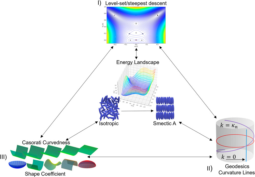
Figure 1. Methodology of the geometric-thermodynamics formulated (Section 2) and implemented (Section 3) in this paper. The central energy landscape corresponding to the direct I-SmA transition is characterized using three geometric methods (I) level sets/steepest descent/critical points, (II) geodesics and curvature lines, and (III) shape and Casorati curvedness analysis; the bottom left shows changes in shape from cup (left), to rut, saddle, ridge, and cap (right) and changes in the degree of curvedness for a rut patch (left) into a flat plane. The outer arrows show the connection and integration of the three calculations.
In (I), at the upper vertex from Figure 1, the critical points (dots) of the surface (maxima, minima, and saddles) are determined as a function of changes in temperature using level-set curves and curves of the steepest descent. The closed loops in the former allow the detection of minima/maxima and saddles, and the signs of the gradient curves differentiate the stable from the unstable. In addition, saddles in the level sets are unstable points. These calculations are guided and validated using the powerful index theorem of polynomials, yielding a conservation equation for the number of maxima
Describing the shape using the dimensionless normalized shape coefficient
This work builds on the fundamental studies on the self-assembled smectic phase transition (Pleiner et al., 2000; Mukherjee et al., 2001; Abukhdeir, 2009; Abukhdeir and Rey, 2009b; Mukherjee, 2021). The particular objectives of this paper are the following:
• Characterize the energy landscape using a simple Monge parametrization in terms of nematic and smectic order parameters, including the number and type of critical points and characteristic trajectories between stable, metastable, and unstable isotropic, nematic, and smectic states as a function of the changing degrees of quenching from the isotropic state.
• Use classical curvatures (Gaussian and mean) and new soft matter geometric methods (shape coefficient and Casorati curvedness) to shed light on where saddles and cusps are located and their curvedness, thus providing a broad picture of the energy landscape.
• Integrate thermodynamic stability, polynomial-based charge conservation methods, and geometric methods.
• Detect and characterize unstable nematic and metastable plastic crystal states that emerge at medium and large degrees of quenching.
The remainder of this paper is organized as follows: Section 2 presents the OPs, Landau free energy (Section 2.1), geometric thermodynamics (Section 2.2), and computational methods (Section 2.3). Section 3 presents the results and discussion. Section 4 summarizes the key findings, their significance, and the novelty of the geometric approach.
The SmA LC phase has partial 1D positional and orientational order. Two order parameters, the orientational order parameter Q and the positional order parameter
The theoretical characterization of the partial orientational alignment in LCs is described by an orientation distribution function, the tensor order parameter Q (De Gennes and Prost, 1993), which is as follows:
where n, m, and l are the molecular unit vectors and I is the unit tensor. The Q tensor is expressed in terms of the orthonormal director triad (n, m, and l), which are the eigenvectors of Q that describe the molecular axes and the scalar moduli
where
In addition to the orientational organization, due to its lamellar configuration and the periodic structure of the uniaxial SmA phase, a one-dimensional positional order parameter is required, and the complex wave vector
Then, a free-energy functional of the smectic positional order,
In the simplest case, the I-SmA transition is captured by the free-energy contributions of the form
The well-established models have been formulated and used to describe the I-SmA transition, including non-direct transitions (Pleiner et al., 2000; Abukhdeir and Rey, 2009b; Nandi et al., 2012; Pevnyi et al., 2014; Izzo and De Oliveira, 2019; Mukherjee, 2021; Paget et al., 2022). These models include the nematic and smectic contributions (Eqs. 2.2, 2.4, and 2.5) and consolidate the final total free-energy density using coupling terms (
Considering Equation 2.6, assuming a spatially homogenous system, and performing reparameterization (see Supplementary Appendix A1), we find the following governing free energy density
where
The possible states are obtained by the minimization of the homogeneous free energy in Equation 2.7 concerning the two non-conserved OPs
The isotropic-liquid state is characterized by the absence of positional and orientational orders, the nematic LC possesses only average molecular orientation, the plastic crystal phase (characterized by the density wave) describes a material with positional order and very small-to-none orientational order, and the smectic A LC exhibits positional and orientational orders (Oswald and Pieranski, 2005a; Oswald and Pieranski, 2005b; De Gennes, 2007; Demus et al., 2008a; DiLisi, 2019; Mukherjee, 2021). We note that the density wave behavior, designated as the plastic crystal state in this study, has been reported even for some rod-like systems (Kyrylyuk et al., 2011; Liu et al., 2014; Sato et al., 2023). In this work, the metastable plastic crystal emerges at deep quenches when the isotropic state becomes unstable, the nematic and coupling energies vanish, and the stable phase is SmA. Similarly, since
In this section, we investigate the surface geometry of the energy landscape
Next, we briefly mention the basic argument to keep all critical points, forgoing complex mathematical details. For instance, the time-dependent Ginzburg–Landau model (Popa-Nita, 1999) provides a quantitative study of the spatiotemporal evolution of thermodynamic behaviors on a non-conserved OPs vector
where
Since the two-OP model considered in this study is of quartic order in each of the parameters, a proliferation of critical points and a complex energy landscape are expected. Hence, tools that set upper limits on the number and type of critical points are essential to achieving or enhancing tractability. In this section, we formulate an approach tailored to the I-SmA transition, keeping the complex mathematics to a minimum.
Let
The number of critical points
Here, the index of the free-energy polynomial of Equation 2.7 was computed as
In addition to the index
The gradient then contains the direction of the greatest change of
The energy landscape
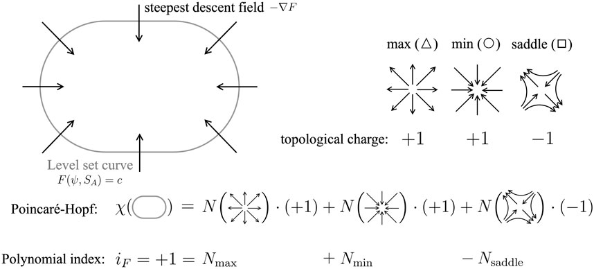
Figure 2. Schematic of the first family of the free-energy landscape
Figure 2 presents the connection between the polynomial index and the level set and steepest descent curves. By assigning topological charges to the critical points based on their nondegeneracy, the polynomial index is constructed. Each nondegenerate point is then linked to the expected local behavior of the gradient vector.
The lines of curvature are computed by solving a set of equations defined by the coefficients of the first (g) and second (b) fundamental forms, as shown in Supplementary Appendix A2 (Maekawa, 1996; Farouki, 1998). The LOC have been used to describe the relationship between entropy production in membranes and interfaces (Wang et al., 2020) and the curvature of isotropic–smectic interfaces under self-organization (equilibrium) and self-assembly (dynamic) states (Vitral et al., 2019) using an orthonormal network. These LOC applied to the free-energy landscape describe the change in the order parameters with respect to the arc-length
or
where
Under our free-energy framework
where E, A, and G are the first fundamental form coefficients,
In this section, we provide details of the Casorati curvature
Classical curvature concepts, in addition to the Casorati curvature
The non-dimensionality of the shape coefficient condenses information that allows it to classify the local shape into simple geometries within the normalized range
The primary fundamental shapes are then generalized with
In this work, we sought detailed information of the phase ordering as the quenching degree increases from the highest possible temperature for the existence of the SmA phase. We found that it is possible to classify the ordering and geometry by defining three quenching regimes: shallow quench, middle quench, and deep quench (with three temperatures corresponding to each of them, as listed in Table 2). As the degree of quenching increased, the isotropic phase lost stability, while the SmA gained stability, and a number of saddle nodes and supercritical bifurcations emerged at the boundaries of these quench regimes. Given the nonlinearities and OP couplings in the energy density and the differential geometry quantities, high-performance computational techniques were developed, applied, and tested when exact data were available, and high fidelity was demonstrated. Stability, accuracy, and dispersion criteria were implemented according to the standard numerical methods. The validation of our results was established using previous studies (Urban et al., 2005; Abukhdeir and Rey, 2008; Coles and Strazielle, 2011). As mentioned in the introduction, a well-characterized member of the n-cyanobiphenyl family (12CB) has been chosen as the study case for its I-SmA transition behavior (see Supplementary Appendix A4).
The calculation sequence was as follows: (1) level sets and steepest descent curves were obtained with (i) the complete solution of Equation 2.7 at different temperatures for the phases in Equation 2.8 using the stability criteria in Section 2.2.1, which categorizes the critical points that are bound by the number
In this paper, we present a complete description and characterization of the energy landscape of the isotropic–smectic A transition using a two-non-conserved order parameter version of the Landau–de Gennes model for the following reasons: (i) the kinetics of phase transformations for non-conserved order parameters is dependent on stable, metastable, and unstable critical points of free energy (Tuckerman and Bechhoefer, 1992; De Luca and Rey, 2003; De Luca and Rey, 2004); this point is briefly elaborated at the beginning of Section 2.2; (ii) in the case of phase transformation by propagating fronts, where a stable phase replaces an unstable phase, non-monotonic ordering structures appear at the interface due to the presence of various critical points (Tuckerman and Bechhoefer, 1992); (iii) in the case of drop formation of a stable phase in a metastable matrix, one can expect thin film-like layers with intermediate degrees of order between the droplet phase and matrix (Abukhdeir and Rey, 2009a); (iv) interfacial processes as in a LC drop couple shape-bulk and surface structure-size due to orientational order (Rey, 2000; Rey and Denn, 2002; Rey, 2004a; Rey, 2004b; Rey, 2006). In view of these phenomena, we do not neglect metastable and unstable ordering states, such as nematic or plastic (density wave) phases, as previously suggested (Saunders et al., 2007). How exactly they will manifest themselves under nucleation and growth and spinodal transformation of the isotropic phase into the SmA phase will be examined in future work and is outside the scope of this paper.
Figure 3 presents the orientational and positional order phase diagram as a function of temperature T obtained by solving Equation 2.7 with 12CB material parameters (Supplementary Appendix A4). Subscripts on the OPs denote stable (s), unstable (u), and metastable (m); superscripts denote larger
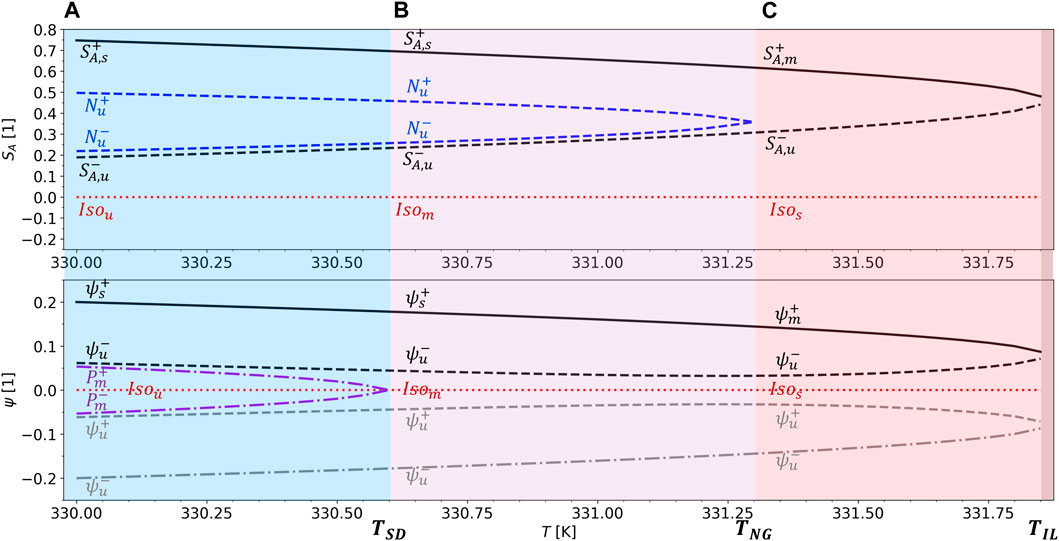
Figure 3. Positional
The phases in the deep quench (light blue region in Figure 2) to the spinodal decomposition region are the following:
•
•
•
•
•
•
Here, the SD region exhibits an unstable isotropic state and a stable SmA. In addition, we find a metastable plastic region. This region exists for
The phases in the middle quench (light purple region in Figure 2) to the nucleation and growth region are the following:
•
•
•
•
•
In the ND region, the isotropic state is metastable and SmA is stable, as in the SD region, in addition to the unstable smectic and nematic phases. However, the density wave is no longer present as it vanishes at the temperature
The phases in the shallow quench (light red region in Figure 2) are the following:
•
•
•
•
At shallow quenches, the isotropic phase is now stable, while SmA is only metastable. In addition, the unstable smectic state remains, but the nematic loop closes and vanishes at the temperature TNG. This region is then defined by
The deep quench is characterized by the strong stability and presence of the expected smectic A phase and by a supercritical bifurcation (Oswald and Pieranski, 2005a) or plastic loop since it belongs to the metastable plastic crystal phase, where mirror symmetry is broken at the temperature
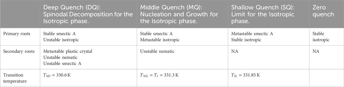
Table 1. Summary of stable, unstable, and metastable states in each quench zone and their key temperatures as presented in Figure 2.
The computed energy landscape has a critical root population that decreases exactly as predicted by the polynomial index theorem (Eq. 2.12; Figure 2) as the temperature increases. This is summarized in Table 2, where the number of nondegenerate points is included along with their type and the index value for each quench zone (see (2.12)).
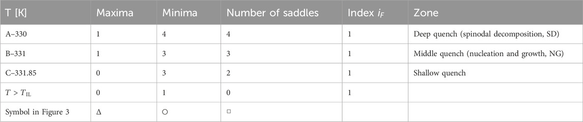
Table 2. Number and types of critical points on the phase diagram for different temperatures and their indexes; the three cases presented in Figure 2 correspond to the three quench zones; and one for the complete isotropic phase transition. The symbol style used for each of them is kept constant throughout the paper. Numerical results are in exact agreement with the polynomial index theorem (Eq. 2.12).
The bounds in Equations 2.10–2.11 provide stability boundaries that do not necessarily mean a phase transition line but present the possible real physical phases that can be displayed within that range given the first-order nature of this transition (Mukherjee et al., 2001). Thus, the phase transition line was found by looking for a metastability–stability exchange of the I-SmA phases using level sets and computing the temperature at which both phases present the same energy level. This temperature,
Figure 4 represents the
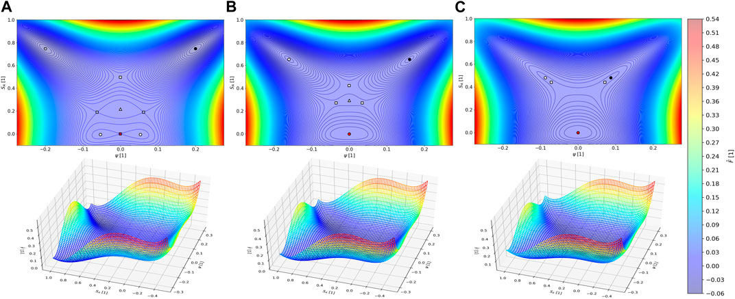
Figure 4. Energy landscape constructed with the positional
Figure 5 presents the level-set curves and the steepest descent lines (see Section 2.2.2), including the critical points projected on the dimensionless energy surface
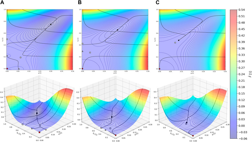
Figure 5.
In partial summary, the level-sets/steepest descent lines show the main features of the energy landscape; the number, location, and type of critical points; and the basin of attraction of SmA under spinodal and nucleation and growth conditions.
Figure 6 shows the 2D projection and 3D plot of the LOC network on the energy landscape
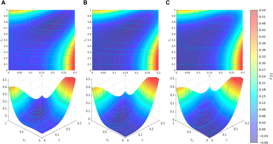
Figure 6. Lines of curvature projected on the
The maximum curvature (magenta) lines on the top left and bottom right closely follow the energy contours, corresponding to high
Figure 7 shows the projected geodesic lines of the energy landscape, computed by solving Equation 2.19 for the temperatures belonging to the three quench zones listed in Table 1 with the method provided in Supplementary Appendix A2. The geodesic family origin is the isotropic state that changes stability from unstable (A) to metastable (B) to stable (C), as seen in Figure 4. The lines minimize the path length and are therefore significant directions for phase changes. These lines show an expanding funnel whose centerline (purple) connects the two primary I-SmA phases. This line, which resembles the MEP introduced in Section 2.2.2, follows the minimum-curvature tendency designated in Figure 6 by the magenta lines. In addition, this phase-connecting geodesic becomes straighter as the depth quench is increased, achieving essentially a straight line in (A), and it starts to bend in the direction of a greater change in energy as the shallow quench (C) is reached. Another important observation is that the change in shape, direction, and bending are reflected in the LOC as the quench regime changes, as opposed to what the geodesics show in this figure.
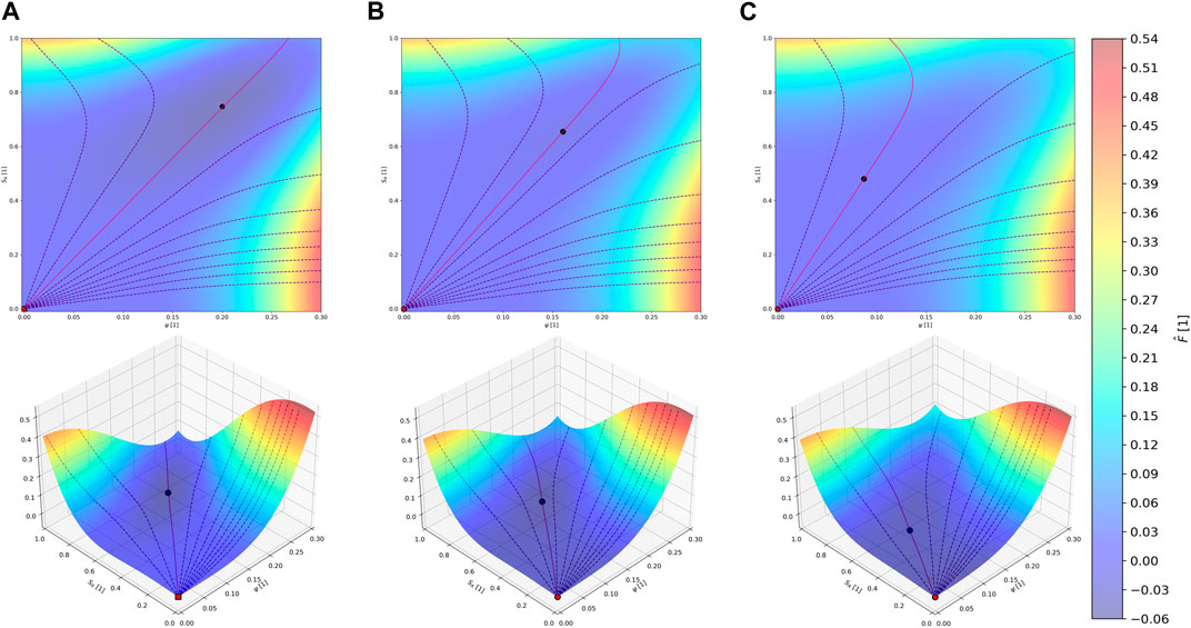
Figure 7. Geodesics superimposed on the
Figure 8 shows the Casorati
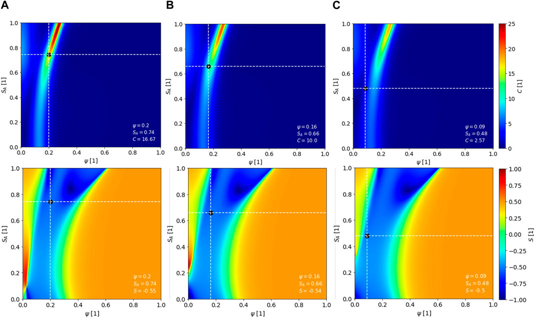
Figure 8. Casorati curvature
The Casorati curvature presents major activity along the zone where the critical points move as the temperature varies. It can be noted that the Casorati curvature decreases as the quench depth decreases, which follows a trend toward the isotropic transition, where both order parameters are zero and the energy surface is planar and, hence,
We now search for the distinguished feature(s) of the shape
• Spinodal decomposition mode:
• Nucleation and growth mode:
• Shallow quench mode:
Figure 8 (bottom) shows another distinguishing feature of the shape index, with the blue concave-up (ridge) domain describing a bent channel that narrows and widens as the order increases. The outer red domains indicate unstable or concave-down (cap) states, and the green boundaries are saddle-like shapes. Hence, the shape landscape for smectic phases follows the previously established rules (Wang et al., 2020) of shape coexistence, where moving from left to right in each panel from Figure 8 (bottom), we find the following:
where saddles are needed to separate minima from maxima, which is in agreement with the polynomial theorem for critical point index
Figure 9 takes the geodesics presented in Figure 7 and projects them on the Casorati and shape coefficient heatmaps from Figure 8 for each temperature according to the three quenching zones listed in Table 1.
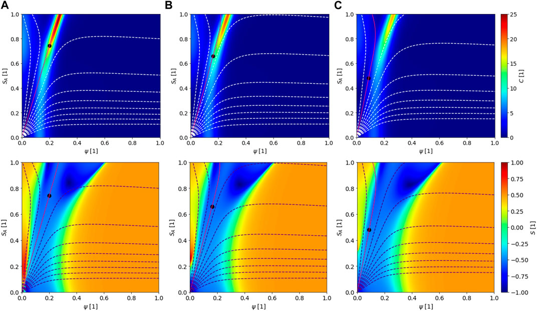
Figure 9. Geodesics projected on the Casorati curvature
The main features gleaned from the Casorati-I-SmA geodesic correlations from Figure 9 (top) are the following:
• The intersection of the geodesic with the high curvedness Casorati tube occurs at high
where the subscripts
• The I-SmA geodesics for NG and SD modes largely avoid the higher Casorati curvatures, indicating paths of lower curvatures.
The main features gleaned from shape coefficient-I-SmA geodesic correlations from Figure 9 (bottom) are as follows:
• The geodesic path remains well-contained in the shape index channel comprehending ruts and trough concave-up shapes, except at low OP and low-temperature values, where saddle-like (green areas close to the origin) and concave-down (red areas close to the origin) shapes arise.
• The development of SmA droplets that may form from an intermediate quench into the NG mode starts with a
Figure 10 integrates the curve families on the energy landscape corresponding to the SD quench regime
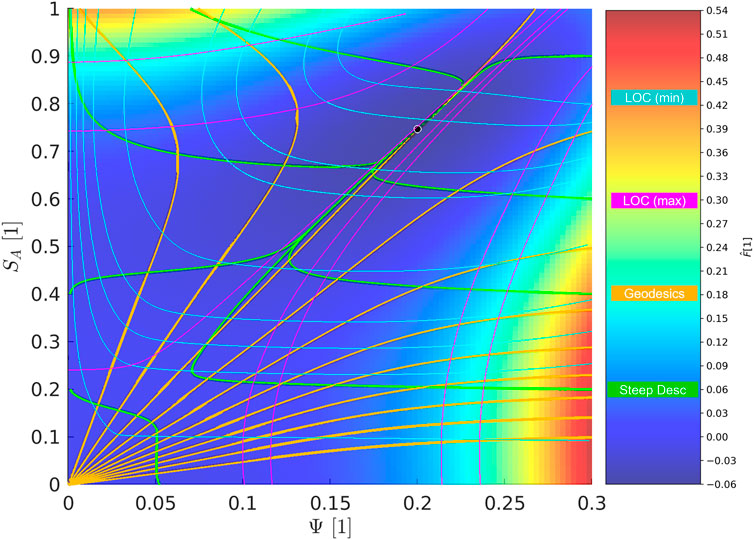
Figure 10.
In this paper, we developed, implemented, and tested a novel computational geometrical method that complements classical liquid crystal phase transition modeling for the complex case of two-order-parameter symmetry breaking. This approach uses complementary geometric schemes to link the thermodynamic energy landscape of the isotropic-to-smectic A liquid crystal direct phase transition with novel soft-matter geometric metrics such as the Casorati curvature and shape coefficient. We summarize the results and their significance as follows:
1. A previously presented and comprehensive study of the Landau–de Gennes free-energy model (De Gennes and Prost, 1993; Pleiner et al., 2000; Larin, 2004; Oswald and Pieranski, 2005b; Donald et al., 2006; Biscari et al., 2007; Abukhdeir and Rey, 2009b; Nandi et al., 2012; Izzo and De Oliveira, 2019) for the direct isotropic-to-smectic A transition with well-known material properties (Urban et al., 2005; Abukhdeir and Rey, 2008; Coles and Strazielle, 2011) formed the basis of the theory and computational modeling characterization of phase ordering with two non-conserved order parameters.
2. The Landau free-energy landscape was obtained using explicit Monge surface parametrization as a function of orientational and positional orders, allowing the deployment of, in a simple manner, differential geometry calculations (Eq. 2.7)
3. The index polynomial theorem (Eq. 2.12) for the number of critical roots as a function of quench depth revealed the importance of saddle roots in the spinodal and nucleation and growth region; without the knowledge of parametric free-energy coefficient data, the theorem shows that the maximum number of critical roots is
4. Using high-performance computing and high-fidelity numerical methods for nonlinear algebraic and differential equations, the following curve families were calculated (Sections 3.2 and 3.3): level-set-steepest descent and geodesic-principal curvatures. These special curves revealed the location of critical points already predicted by the index theorem, directions of small and large curvatures, and minimal length connections between isotropic and smectic roots. In particular, linear geodesics joining isotropic and smectic states in nucleation and growth and spinodal quenches revealed phase transformation paths. The level-set curves around stable roots were elliptical, indicating anisotropy originating from the Landau free-energy polynomial.
5. The emergence of metastable plastic crystals at deep quenches and unstable nematic states at deep and intermediate quenches was characterized, and their annihilation through supercritical and saddle-node bifurcation was captured, re-emphasizing results from the index polynomial theorem. The relevance of the nematic or plastic order at the interfaces of smectic A drops in an isotropic matrix was pointed out.
6. Previously presented measures of shape and curvedness (Casorati) in soft-matter materials were used (Section 3.4) to characterize the energy landscape with purely geometric measures instead of order parameter coordinates. The calculations were integrated with the curve families, showing consistency and revealing that the Casorati landscape is a bent, higher-curved tube embedded in a low-curvedness matrix; the tube is well-fitted with a power law function. The smectic A root resides inside this tube and moves downward as the temperature increases. The shape coefficient landscape is characterized by a wide channel of concave-up shapes separated from an area of concave-down shapes by saddle-like interfaces, which is in agreement with shape coexistence phenomena.
7. Plotting all the curve families (point 4 above) in the energy landscape, we find that at large quench, the isotropic-to-smectic A geodesic is an attractor for maximal lines of curvature and curves of the steepest descent, explaining the stability of the smectic A state.
The combination of parameter-free predictions from polynomial theorems with the computational geometry of the free-energy landscape contributes to the evolving understanding and characterization of the isotropic-to-smectic A transition, which is of high interest to biological colloidal liquid crystals, such as in the precursors to the mussel byssus (Renner-Rao et al., 2019; Harrington and Fratzl, 2021; Jehle et al., 2021) through droplet nucleation/growth and colloidal impingement. We demonstrated that the presence of two non-conserved order parameters creates challenges in equilibrium spatially homogeneous simulations, but how time-dependent processes such as droplet growth resolve the couplings of shape–size–structure–interface remains to be elucidated in future work by building on the present results and methods.
Data related to this work will be made available by request to the authors. Requests to access the datasets should be directed to ADR, YWxlamFuZHJvLnJleUBtY2dpbGwuY2E=.
DZ: writing–original draft, conceptualization, data curation, formal analysis, investigation, methodology, software, validation, visualization, and writing–review and editing. ZW: conceptualization, writing–review and editing, validation, and methodology. ND: conceptualization, supervision, and writing–review and editing. MH: conceptualization, supervision, and writing–review and editing. AR: conceptualization, validation, writing–review and editing, formal analysis, funding acquisition, project administration, resources, and supervision.
The author(s) declare that financial support was received for the research, authorship, and/or publication of this article. This work was supported by the Fonds de Recherche du Québec (FRQNT) (2021-PR-284991) and the Natural Science and Engineering Research Council of Canada (NSERC) (#223086). Author DUZC thanks Consejo Nacional de Humanidades, Ciencia y Tecnología (CONAHCYT) (853563), and McGill Engineering Doctoral Award (MEDA) scholarships for financial support.
The authors acknowledge Digital Research Alliance of Canada (ID 4700) for computational resources and technical support.
The authors declare that the research was conducted in the absence of any commercial or financial relationships that could be construed as a potential conflict of interest.
All claims expressed in this article are solely those of the authors and do not necessarily represent those of their affiliated organizations, or those of the publisher, the editors, and the reviewers. Any product that may be evaluated in this article, or claim that may be made by its manufacturer, is not guaranteed or endorsed by the publisher.
The Supplementary Material for this article can be found online at: https://www.frontiersin.org/articles/10.3389/frsfm.2024.1359128/full#supplementary-material
Abbena, E., Salamon, S., and Gray, A. (2017). Modern differential geometry of curves and surfaces with Mathematica. China: CRC Press.
Abukhdeir, N. M. (2009). Growth, dynamics, and texture modeling of the lamellar smectic-A liquid crystalline transition. Doctor of Philosophy. Canada: McGill University.
Abukhdeir, N. M., and Rey, A. D. (2008). Simulation of spherulite growth using a comprehensive approach to modeling the first-order isotropic/smectic-A mesophase transition. arXiv Prepr. arXiv:0807.4525. doi:10.48550/arXiv.0807.4525
Abukhdeir, N. M., and Rey, A. D. (2009a). Metastable nematic preordering in smectic liquid crystalline phase transitions. Macromolecules 42, 3841–3844. doi:10.1021/ma900796b
Abukhdeir, N. M., and Rey, A. D. (2009b). Nonisothermal model for the direct isotropic/smectic-A liquid-crystalline transition. Langmuir 25, 11923–11929. doi:10.1021/la9015965
Abukhdeir, N. M., and Rey, A. D. (2009c). Shape-dynamic growth, structure, and elasticity of homogeneously oriented spherulites in an isotropic/smectic-A mesophase transition. Liq. Cryst. 36, 1125–1137. doi:10.1080/02678290902878754
Aguilar Gutierrez, O. F., and Rey, A. D. (2018). Extracting shape from curvature evolution in moving surfaces. Soft Matter 14, 1465–1473. doi:10.1039/c7sm02409f
Bellini, T., Clark, N. A., and Link, D. R. (2002). Isotropic to smectic a phase transitions in a porous matrix: a case of multiporous phase coexistence. J. Phys. Condens. Matter 15, S175–S182. doi:10.1088/0953-8984/15/1/322
Berent, K., Cartwright, J. H. E., Checa, A. G., Pimentel, C., Ramos-Silva, P., and Sainz-Díaz, C. I. (2022). Helical microstructures in molluscan biomineralization are a biological example of close packed helices that may form from a colloidal liquid crystal precursor in a twist--bend nematic phase. Phys. Rev. Mater. 6, 105601. doi:10.1103/physrevmaterials.6.105601
Biscari, P., Calderer, M. C., and Terentjev, E. M. (2007). Landau-de Gennes theory of isotropic-nematic-smectic liquid crystal transitions. Phys. Rev. E Stat. Nonlin Soft Matter Phys. 75, 051707. doi:10.1103/physreve.75.051707
Bowick, M. J., Kinderlehrer, D., Menon, G., and Radin, C. (2017). Mathematics and materials, American mathematical soc.
Bradley, P. A. (2019). On the physicochemical control of collagen fibrilligenesis and biomineralization. Doctor of Philosophy. USA: Northeastern University.
Bukharina, D., Kim, M., Han, M. J., and Tsukruk, V. V. (2022). Cellulose nanocrystals' assembly under ionic strength variation: from high orientation ordering to a random orientation. Langmuir 38, 6363–6375. doi:10.1021/acs.langmuir.2c00293
Bunsell, A. R., Joannès, S., and Thionnet, A. (2021). Fundamentals of fibre reinforced composite materials. Germany: CRC Press.
Cai, A., Abdali, Z., Saldanha, D. J., Aminzare, M., and Dorval Courchesne, N.-M. (2023). Endowing textiles with self-repairing ability through the fabrication of composites with a bacterial biofilm. Sci. Rep. 13, 11389. doi:10.1038/s41598-023-38501-2
Chahine, G., Kityk, A. V., Démarest, N., Jean, F., Knorr, K., Huber, P., et al. (2010). Collective molecular reorientation of a calamitic liquid crystal (12CB) confined in alumina nanochannels. Phys. Rev. E 82, 011706. doi:10.1103/physreve.82.011706
Coles, H. J., and Strazielle, C. (2011). The order-disorder phase transition in liquid crystals as a function of molecular structure. I. The alkyl cyanobiphenyls. Mol. Cryst. Liq. Cryst. 55, 237–250. doi:10.1080/00268947908069805
Collings, P. J. (1997). Phase structures and transitions in thermotropic liquid crystals handbook of liquid crystal research.
Collings, P. J., and Goodby, J. W. (2019). Introduction to liquid crystals: chemistry and physics. Germany: Crc Press.
Collings, P. J., and Hird, M. (2017). Introduction to liquid crystals chemistry and physics. Germany: CRC Press.
Copic, M., and Mertelj, A. (2020). Q-tensor model of twist-bend and splay nematic phases. Phys. Rev. E 101, 022704. doi:10.1103/physreve.101.022704
Das, A. K., and Mukherjee, P. K. (2009). Phenomenological theory of the direct isotropic to hexatic-B phase transition. J. Chem. Phys. 130, 054901. doi:10.1063/1.3067425
de Gennes, P. G. (2007). Some remarks on the polymorphism of smectics. Mol. Cryst. Liq. Cryst. 21, 49–76. doi:10.1080/15421407308083313
de Gennes, P.-G., and Prost, J. (1993). The physics of liquid crystals. Oxford: Oxford University Press.
de Luca, G., and Rey, A. D. (2004). Chiral front propagation in liquid-crystalline materials: formation of the planar monodomain twisted plywood architecture of biological fibrous composites. Phys. Rev. E 69, 011706. doi:10.1103/physreve.69.011706
de Luca, G., and Rey, A. D. (2006). Dynamic interactions between nematic point defects in the spinning extrusion duct of spiders. J. Chem. Phys. 124, 144904. doi:10.1063/1.2186640
de Luca, G., and Rey, A. (2003). Monodomain and polydomain helicoids in chiral liquid-crystalline phases and their biological analogues. Eur. Phys. J. E 12, 291–302. doi:10.1140/epje/i2002-10164-3
Demirci, N., and Holland, M. A. (2022). Cortical thickness systematically varies with curvature and depth in healthy human brains. Hum. Brain Mapp. 43, 2064–2084. doi:10.1002/hbm.25776
Demus, D., Goodby, J. W., Gray, G. W., Spiess, H. W., and Vill, V. (2008a). Handbook of liquid crystals.
Demus, D., Goodby, J. W., Gray, G. W., Spiess, H. W., and Vill, V. (2008b). Handbook of liquid crystals, volume 3: high molecular weight liquid crystals. USA: John Wiley and Sons.
Demus, D., Goodby, J. W., Gray, G. W., Spiess, H. W., and Vill, V. (2011). Handbook of liquid crystals, volume 2A: low molecular weight liquid crystals I: calamitic liquid crystals. USA: John Wiley and Sons.
Deng, F., Dang, Y., Tang, L., Hu, T., Ding, C., Hu, X., et al. (2021). Tendon-inspired fibers from liquid crystalline collagen as the pre-oriented bioink. Int. J. Biol. Macromol. 185, 739–749. doi:10.1016/j.ijbiomac.2021.06.173
Dierking, I., and al-Zangana, S. (2017). Lyotropic liquid crystal phases from anisotropic nanomaterials. Nanomater. (Basel) 7, 305. doi:10.3390/nano7100305
Dilisi, G. A. (2019). in An introduction to liquid crystals. Editor J. J. DELUCA (New York: Morgan and Claypool Publishers).
Do Carmo, M. P. (2016). Differential geometry of curves and surfaces: revised and updated. second edition. New York: Courier Dover Publications.
Dogic, Z., and Fraden, S. (2001). Development of model colloidal liquid crystals and the kinetics of the isotropic-smectic transition. Philosophical Trans. R. Soc. a-Mathematical Phys. Eng. Sci. 359, 997–1015. DOI, M. 1981. doi:10.1098/rsta.2000.0814
Doi, M. 2022 Molecular dynamics and rheological properties of concentrated solutions of rodlike polymers in isotropic and liquid crystalline phases. J. Polym. Sci. Polym. Phys. Ed. 19, 229–243. doi:10.1002/pol.1981.180190205
Donald, A. M., Windle, A. H., and Hanna, S. (2006). Liquid crystalline polymers. Cambridge: Cambridge University Press.
Durfee, A., Kronenfeld, N., Munson, H., Roy, J., and Westby, I. (1993). Counting critical points of real polynomials in two variables. Am. Math. Mon. 100, 255–271. doi:10.2307/2324459
Farouki, R. T. (1998). On integrating lines of curvature. Comput. Aided Geom. Des. 15, 187–192. doi:10.1016/s0167-8396(97)00022-8
Fischer, S., and Karplus, M. (1992). Conjugate peak refinement: an algorithm for finding reaction paths and accurate transition states in systems with many degrees of freedom. Chem. Phys. Lett. 194, 252–261. doi:10.1016/0009-2614(92)85543-j
Garti, N., Somasundaran, P., and Mezzenga, R. (2012). Self-assembled supramolecular architectures: lyotropic liquid crystals. USA: John Wiley and Sons.
Golmohammadi, M., and Rey, A. D. (2009). Thermodynamic modelling of carbonaceous mesophase mixtures. Liq. Cryst. 36, 75–92. doi:10.1080/02678290802666218
Golmohammadi, M., and Rey, A. D. (2010). Structural modeling of carbonaceous mesophase amphotropic mixtures under uniaxial extensional flow. J. Chem. Phys. 133, 034903. doi:10.1063/1.3455505
Gorkunov, M., Osipov, M., Lagerwall, J., and Giesselmann, F. (2007). Order-disorder molecular model of the smectic-A–smectic-C phase transition in materials with conventional and anomalously weak layer contraction. Phys. Rev. E 76, 051706. doi:10.1103/physreve.76.051706
Gudimalla, A., Thomas, S., and Zidanšek, A. (2021). Phase behaviour of n-CB liquid crystals confined to controlled pore glasses. J. Mol. Struct. 1235, 130217. doi:10.1016/j.molstruc.2021.130217
Gurevich, S., Soule, E., Rey, A., Reven, L., and Provatas, N. (2014). Self-assembly via branching morphologies in nematic liquid-crystal nanocomposites. Phys. Rev. E 90, 020501. doi:10.1103/physreve.90.020501
Gurin, P., Odriozola, G., and Varga, S. (2021). Enhanced two-dimensional nematic order in slit-like pores. New J. Phys. 23, 063053. doi:10.1088/1367-2630/ac05e1
Han, J. Q., Luo, Y., Wang, W., Zhang, P. W., and Zhang, Z. F. (2015). From microscopic theory to macroscopic theory: a systematic study on modeling for liquid crystals. Archive Ration. Mech. Analysis 215, 741–809. doi:10.1007/s00205-014-0792-3
Han, W., and Rey, A. (1993). Supercritical bifurcations in simple shear flow of a non-aligning nematic: reactive parameter and director anchoring effects. J. Newt. fluid Mech. 48, 181–210. doi:10.1016/0377-0257(93)80070-r
Harrington, M. J., and Fratzl, P. (2021). Natural load-bearing protein materials. Prog. Mater. Sci. 120, 100767. doi:10.1016/j.pmatsci.2020.100767
Hawkins, R. J., and April, E. W. (1983). “Liquid crystals in living tissues,” in Advances in liquid crystals. Editor G. H. BROWN (Germany: Elsevier).
Hormann, K., and Zimmer, J. (2007). On Landau theory and symmetric energy landscapes for phase transitions. J. Mech. Phys. Solids 55, 1385–1409. doi:10.1016/j.jmps.2007.01.004
Idziak, S. H. J., Koltover, I., Davidson, P., Ruths, M., Li, Y., Israelachvili, J. N., et al. (1996). Structure under confinement in a smectic-A and lyotropic surfactant hexagonal phase. Phys. B Condens. Matter 221, 289–295. doi:10.1016/0921-4526(95)00939-6
Izzo, D., and de Oliveira, M. J. (2019). Landau theory for isotropic, nematic, smectic-A, and smectic-C phases. Liq. Cryst. 47, 99–105. doi:10.1080/02678292.2019.1631968
Jackson, K., Peivandi, A., Fogal, M., Tian, L., and Hosseinidoust, Z. (2021). Filamentous phages as building blocks for bioactive hydrogels. ACS Appl. Bio Mater. 4, 2262–2273. doi:10.1021/acsabm.0c01557
Jákli, A., and Saupe, A. (2006). One-and two-dimensional fluids: properties of smectic, lamellar and columnar liquid crystals. New York: CRC Press.
Jehle, F., Priemel, T., Strauss, M., Fratzl, P., Bertinetti, L., and Harrington, M. J. (2021). Collagen pentablock copolymers form smectic liquid crystals as precursors for mussel byssus fabrication. ACS Nano 15, 6829–6838. doi:10.1021/acsnano.0c10457
Khadem, S. A., and Rey, A. D. (2021). Nucleation and growth of cholesteric collagen tactoids: a time-series statistical analysis based on integration of direct numerical simulation (DNS) and long short-term memory recurrent neural network (LSTM-RNN). J. Colloid Interface Sci. 582, 859–873. doi:10.1016/j.jcis.2020.08.052
Khan, B. C., and Mukherjee, P. K. (2021). Isotropic to smectic-A phase transition in taper-shaped liquid crystal. J. Mol. Liq. 329, 115539. doi:10.1016/j.molliq.2021.115539
Knight, D., and Vollrath, F. (1999). Hexagonal columnar liquid crystal in the cells secreting spider silk. Tissue Cell. 31, 617–620. doi:10.1054/tice.1999.0076
Knill, O. (2012). A graph theoretical Poincaré-Hopf theorem. arXiv Prepr. arXiv:1201.1162. doi:10.48550/arXiv.1201.1162
Koenderink, J. J., and van Doorn, A. J. (1992). Surface shape and curvature scales. Image Vis. Comput. 10, 557–564. doi:10.1016/0262-8856(92)90076-f
Kyrylyuk, A. V., Anne van de Haar, M., Rossi, L., Wouterse, A., and Philipse, A. P. (2011). Isochoric ideality in jammed random packings of non-spherical granular matter. Soft Matter 7, 1671–1674. doi:10.1039/c0sm00754d
Lagerwall, J. P. (2016). An introduction to the physics of liquid crystals. Fluids, Colloids Soft Mater. Introd. Soft Matter Phys., 307–340. doi:10.1002/9781119220510.ch16
Larin, E. S. (2004). Phase diagram of transitions from an isotropic phase to nematic and smectic (uniaxial, biaxial) phases in liquid crystals with achiral molecules. Phys. Solid State 46, 1560–1568. doi:10.1134/1.1788795
Lenoble, J., Campidelli, S., Maringa, N., Donnio, B., Guillon, D., Yevlampieva, N., et al. (2007). Liquid− crystalline Janus-type fullerodendrimers displaying tunable smectic− columnar mesomorphism. J. Am. Chem. Soc. 129, 9941–9952. doi:10.1021/ja071012o
Li, C.-Z., Matsuo, Y., and Nakamura, E. (2009). Luminescent bow-tie-shaped decaaryl[60]fullerene mesogens. J. Am. Chem. Soc. 131, 17058–17059. doi:10.1021/ja907908m
Liu, B., Besseling, T. H., Hermes, M., Demirörs, A. F., Imhof, A., and van Blaaderen, A. (2014). Switching plastic crystals of colloidal rods with electric fields. Nat. Commun. 5, 3092. doi:10.1038/ncomms4092
Liu, X., Chen, H., and Ortner, C. (2022). Stability of the minimum energy path. arXiv Prepr. arXiv:2204.00984. doi:10.1007/s00211-023-01391-7
Manolakis, I., and Azhar, U. (2020). Recent advances in mussel-inspired synthetic polymers as marine antifouling coatings. Coatings 10, 653. doi:10.3390/coatings10070653
Massi, F., and Straub, J. E. (2001). Energy landscape theory for Alzheimer's amyloid β-peptide fibril elongation. Proteins Struct. Funct. Bioinforma. 42, 217–229. doi:10.1002/1097-0134(20010201)42:2<217::aid-prot90>3.0.co;2-n
Matthews, J. A., Wnek, G. E., Simpson, D. G., and Bowlin, G. L. (2002). Electrospinning of collagen nanofibers. Biomacromolecules 3, 232–238. doi:10.1021/bm015533u
Milette, J., Toader, V., Soulé, E. R., Lennox, R. B., Rey, A. D., and Reven, L. (2013). A molecular and thermodynamic view of the assembly of gold nanoparticles in nematic liquid crystal. Langmuir 29, 1258–1263. doi:10.1021/la304189n
Miller, W. L. (1925). The method of willard gibbs in chemical thermodynamics. Chem. Rev. 1, 293–344. doi:10.1021/cr60004a001
Mohieddin Abukhdeir, N., and Rey, A. D. (2008a). Defect kinetics and dynamics of pattern coarsening in a two-dimensional smectic-A system. New J. Phys. 10, 063025. doi:10.1088/1367-2630/10/6/063025
Mohieddin Abukhdeir, N., and Rey, A. D. 2008b. Modeling the isotropic/smectic-C tilted lamellar liquid crystalline transition.
Mukherjee, P. K. (2014). Isotropic to smectic-A phase transition: a review. J. Mol. Liq. 190, 99–111. doi:10.1016/j.molliq.2013.11.001
Mukherjee, P. K. (2021). Advances of isotropic to smectic phase transitions. J. Mol. Liq. 340, 117227. doi:10.1016/j.molliq.2021.117227
Mukherjee, P. K., Pleiner, H., and Brand, H. R. (2001). Simple Landau model of the smectic-A-isotropic phase transition. Eur. Phys. J. E 4, 293–297. doi:10.1007/s101890170111
Nandi, B., Saha, M., and Mukherjee, P. K. (2012). Landau theory of the direct smectic-A to isotropic phase transition. Int. J. Mod. Phys. B 11, 2425–2432. doi:10.1142/s0217979297001234
Nesrullajev, A. (2022). Optical refracting properties, birefringence and order parameter in mixtures of liquid crystals: direct smectic A – Isotropic and reverse isotropic – smectic A phase transitions. J. Mol. Liq. 345, 117716. doi:10.1016/j.molliq.2021.117716
Oh, C. S. (1977). Induced smectic mesomorphism by incompatible nematogens. Mol. Cryst. Liq. Cryst. 42, 1–14. doi:10.1080/15421407708084491
Oswald, P., and Pieranski, P. (2005a). Nematic and cholesteric liquid crystals: concepts and physical properties illustrated by experiments. China: CRC Press.
Paget, J., Alberti, U., Mazza, M. G., Archer, A. J., and Shendruk, T. N. (2022). Smectic layering: Landau theory for a complex-tensor order parameter. J. Phys. A Math. Theor. 55, 354001. doi:10.1088/1751-8121/ac80df
Palffy-Muhoray, P. (1999). Dynamics of filaments during the isotropic-smectic A phase transition. J. Nonlinear Sci. 9, 417–437. doi:10.1007/s003329900075
Petrov, A. G. (2013). Flexoelectricity in lyotropics and in living liquid crystals. Flexoelectricity Liq. Cryst. theory, Exp. Appl. World Sci. doi:10.1142/9781848168008_0007
Pevnyi, M. Y., Selinger, J. V., and Sluckin, T. J. (2014). Modeling smectic layers in confined geometries: order parameter and defects. Phys. Rev. E Stat. Nonlin Soft Matter Phys. 90, 032507. doi:10.1103/physreve.90.032507
Picken, S. J. (1990). Orientational order in aramid solutions determined by diamagnetic susceptibility and birefringence measurements. Macromolecules 23, 464–470. doi:10.1021/ma00204a019
Pleiner, H., Mukherjee, P. K., and Brand, H. R. (2000). Direct transitions from isotropic to smectic phases. Proc. Freiburger Arbeitstagung Flussigkristalle, P59.
Popa-Nita, V. (1999). Statics and kinetics at the nematic-isotropic interface in porous media. Eur. Phys. J. B-Condensed Matter Complex Syst. 12, 83–90. doi:10.1007/s100510050981
Popa-Nita, V., and Sluckin, T. J. (2007). Waves at the nematic-isotropic interface: nematic-non-nematic and polymer-nematic mixtures. Netherlands: Springer, 253–267.
Pouget, E., Grelet, E., and Lettinga, M. P. (2011). Dynamics in the smectic phase of stiff viral rods. Phys. Rev. E Stat. Nonlin Soft Matter Phys. 84, 041704. doi:10.1103/physreve.84.041704
Quevedo, H., Quevedo, M. N., and Sánchez, A. (2022). Geometrothermodynamics of van der Waals systems. J. Geometry Phys. 176, 104495. doi:10.1016/j.geomphys.2022.104495
Quevedo, H., Sánchez, A., Taj, S., and Vázquez, A. (2011). Phase transitions in geometrothermodynamics. General Relativ. Gravit. 43, 1153–1165. doi:10.1007/s10714-010-0996-2
Quevedo, H., Sánchez, A., and Vázquez, A. (2008). Invariant geometry of the ideal gas. arXiv Prepr. arXiv:0811.0222.
Renner-Rao, M., Clark, M., and Harrington, M. J. (2019). Fiber Formation from liquid crystalline collagen vesicles isolated from mussels. Langmuir 35, 15992–16001. doi:10.1021/acs.langmuir.9b01932
Rey, A. D. (1995). Bifurcational analysis of the isotropic-discotic nematic phase transition in the presence of extensional flow. Liq. Cryst. 19, 325–331. doi:10.1080/02678299508031988
Rey, A. D. (2000). Viscoelastic theory for nematic interfaces. Phys. Rev. E 61, 1540–1549. doi:10.1103/physreve.61.1540
Rey, A. D. (2004a). Interfacial thermodynamics of polymeric mesophases. Macromol. theory simulations 13, 686–696. doi:10.1002/mats.200400030
Rey, A. D. (2004b). Thermodynamics of soft anisotropic interfaces. J. Chem. Phys. 120, 2010–2019. doi:10.1063/1.1635357
Rey, A. D. (2006). Mechanical model for anisotropic curved interfaces with applications to surfactant-laden Liquid− liquid crystal interfaces. Langmuir 22, 219–228. doi:10.1021/la051974d
Rey, A. D. (2010). Liquid crystal models of biological materials and processes. Soft Matter 6, 3402–3429. doi:10.1039/b921576j
Rey, A. D., and Denn, M. M. (2002). Dynamical phenomena in liquid-crystalline materials. Annu. Rev. Fluid Mech. 34, 233–266. doi:10.1146/annurev.fluid.34.082401.191847
Rey, A. D., and Herrera-Valencia, E. E. (2012). Liquid crystal models of biological materials and silk spinning. Biopolymers 97, 374–396. doi:10.1002/bip.21723
Rey, A. D., Herrera-Valencia, E. E., and Murugesan, Y. K. (2013). Structure and dynamics of biological liquid crystals. Liq. Cryst. 41, 430–451. doi:10.1080/02678292.2013.845698
Salamonczyk, M., Zhang, J., Portale, G., Zhu, C., Kentzinger, E., Gleeson, J. T., et al. (2016). Smectic phase in suspensions of gapped DNA duplexes. Nat. Commun. 7, 13358. doi:10.1038/ncomms13358
Sato, C., Takeda, T., Dekura, S., Suzuki, Y., Kawamata, J., and Akutagawa, T. (2023). Chiral plastic crystal of solid-state dual rotators. Cryst. Growth and Des. 23, 5889–5898. doi:10.1021/acs.cgd.3c00495
Saunders, K., Hernandez, D., Pearson, S., and Toner, J. (2007). Disordering to order: de Vries behavior from a Landau theory for smectic phases. Phys. Rev. Lett. 98, 197801. doi:10.1103/physrevlett.98.197801
Schimming, C. D., Viñals, J., and Walker, S. W. (2021). Numerical method for the equilibrium configurations of a Maier-Saupe bulk potential in a Q-tensor model of an anisotropic nematic liquid crystal. J. Comput. Phys. 441, 110441. doi:10.1016/j.jcp.2021.110441
Selinger, J. V. (2016). Introduction to the theory of soft matter: from ideal gases to liquid crystals. Germany: Springer.
Sonnet, A. M., and Virga, E. G. (2012). Dissipative ordered fluids: theories for liquid crystals. Germany: Springer Science and Business Media.
Soulé, E. R., Lavigne, C., Reven, L., and Rey, A. D. (2012a). Multiple interfaces in diffusional phase transitions in binary mesogen-nonmesogen mixtures undergoing metastable phase separations. Phys. Rev. E 86, 011605. doi:10.1103/physreve.86.011605
Soulé, E. R., Milette, J., Reven, L., and Rey, A. D. (2012b). Phase equilibrium and structure formation in gold nanoparticles—nematic liquid crystal composites: experiments and theory. Soft Matter 8, 2860–2866. doi:10.1039/c2sm07091j
Soulé, E. R., Reven, L., and Rey, A. D. (2012c). Thermodynamic modelling of phase equilibrium in nanoparticles–nematic liquid crystals composites. Mol. Cryst. Liq. Cryst. 553, 118–126. doi:10.1080/15421406.2011.609447
Soule, E. R., and Rey, A. D. (2011). A good and computationally efficient polynomial approximation to the Maier–Saupe nematic free energy. Liq. Cryst. 38, 201–205. doi:10.1080/02678292.2010.539303
Soule, E. R., and Rey, A. D. (2012). Modelling complex liquid crystal mixtures: from polymer dispersed mesophase to nematic nanocolloids. Mol. Simul. 38, 735–750. doi:10.1080/08927022.2012.669478
Stewart, I. W. (2019). The static and dynamic continuum theory of liquid crystals: a mathematical introduction. Germany: Crc Press.
Tortora, M., and Jost, D. (2021). Morphogenesis and self-organization of persistent filaments confined within flexible biopolymeric shells. arXiv Prepr. doi:10.48550/arXiv.2107.02598
Tuckerman, L. S., and Bechhoefer, J. (1992). Dynamical mechanism for the formation of metastable phases: the case of two nonconserved order parameters. Phys. Rev. A 46, 3178–3192. doi:10.1103/physreva.46.3178
Turek, D. E., Simon, G. P., and Tiu, C. (2020). “Relationships among rheology, morphology, and solid-state properties in thermotropic liquid-crystalline polymers,” in Handbook of applied polymer processing technology (Germany: CRC Press).
Urban, S., Przedmojski, J., and Czub, J. (2005). X-ray studies of the layer thickness in smectic phases. Liq. Cryst. 32, 619–624. doi:10.1080/02678290500116920
Viney, C. (2004). Self-assembly as a route to fibrous materials: concepts, opportunities and challenges. Curr. Opin. Solid State and Mater. Sci. 8, 95–101. doi:10.1016/j.cossms.2004.04.001
Vitral, E., Leo, P. H., and Vinals, J. (2019). Role of Gaussian curvature on local equilibrium and dynamics of smectic-isotropic interfaces. Phys. Rev. E 100, 032805. doi:10.1103/physreve.100.032805
Vitral, E., Leo, P. H., and Vinals, J. (2020). Model of the dynamics of an interface between a smectic phase and an isotropic phase of different density. Phys. Rev. Fluids 5, 073302. doi:10.1103/physrevfluids.5.073302
Waite, J. H., and Harrington, M. J. (2022). Following the thread: Mytilus mussel byssus as an inspired multi-functional biomaterial. Can. J. Chem. 100, 197–211. doi:10.1139/cjc-2021-0191
Wales, D. J. (2018). Exploring energy landscapes. Annu. Rev. Phys. Chem. 69, 401–425. doi:10.1146/annurev-physchem-050317-021219
Wang, H. Y., Wang, Y. Z., Tsakalakos, T., Semenovskaya, S., and Khachaturyan, A. G. (1996). Indirect nucleation in phase transformations with symmetry reduction. Philosophical Mag. a-Physics Condens. Matter Struct. Defects Mech. Prop. 74, 1407–1420. doi:10.1080/01418619608240732
Wang, Z., Servio, P., and Rey, A. D. (2020). Rate of entropy production in evolving interfaces and membranes under astigmatic kinematics: shape evolution in geometric-dissipation landscapes. Entropy 22, 909. doi:10.3390/e22090909
Wang, Z., Servio, P., and Rey, A. D. (2022a). Complex nanowrinkling in chiral liquid crystal surfaces: from shaping mechanisms to geometric statistics. Nanomaterials 12, 1555. doi:10.3390/nano12091555
Wang, Z., Servio, P., and Rey, A. D. (2023a). Geometry-structure models for liquid crystal interfaces, drops and membranes: wrinkling, shape selection and dissipative shape evolution. Soft Matter 19, 9344–9364. doi:10.1039/d3sm01164j
Wang, Z., Servio, P., and Rey, A. D. (2023b). Pattern formation, structure and functionalities of wrinkled liquid crystal surfaces: a soft matter biomimicry platform. Front. Soft Matter 3, 1123324. doi:10.3389/frsfm.2023.1123324
Wang, Z., Servio, P., and Rey, A. (2022b). Wrinkling pattern formation with periodic nematic orientation: from egg cartons to corrugated surfaces. Phys. Rev. E 105, 034702. doi:10.1103/physreve.105.034702
Ward, I. (1993). New developments in the production of high modulus and high strength flexible polymers. Orientational Phenomena in Polymers. Germany: Springer, 103–110.
Wojcik, M., Lewandowski, W., Matraszek, J., Mieczkowski, J., Borysiuk, J., Pociecha, D., et al. (2009). Liquid-crystalline phases made of gold nanoparticles. Angew. Chem. Int. Ed. 48, 5167–5169. doi:10.1002/anie.200901206
Zaluzhnyy, I. A., Kurta, R., Sprung, M., Vartanyants, I. A., and Ostrovskii, B. I. (2022). Angular structure factor of the hexatic-B liquid crystals: bridging theory and experiment. Soft Matter 18, 783–792. doi:10.1039/d1sm01446c
Zannoni, C. (2022). Liquid crystals and their computer simulations. Germany: Cambridge University Press.
Zhang, Z., Yang, X., Zhao, Y., Ye, F., and Shang, L. (2023). Liquid crystal materials for biomedical applications. Adv. Mater. 35, 2300220. doi:10.1002/adma.202300220
Keywords: liquid crystals, smectic A, phase transition, energy landscape, shape coefficient, free energy, Landau–de Gennes
Citation: Zamora Cisneros DU, Wang Z, Dorval Courchesne N-M, Harrington MJ and Rey AD (2024) Geometric modeling of phase ordering for the isotropic–smectic A phase transition. Front. Soft Matter 4:1359128. doi: 10.3389/frsfm.2024.1359128
Received: 20 December 2023; Accepted: 16 April 2024;
Published: 21 May 2024.
Edited by:
Frank Alexis, Universidad San Francisco de Quito, EcuadorReviewed by:
Anne-laure Fameau, Institut National de recherche pour l’agriculture, l’alimentation et l’environnement (INRAE), FranceCopyright © 2024 Zamora Cisneros, Wang, Dorval Courchesne, Harrington and Rey. This is an open-access article distributed under the terms of the Creative Commons Attribution License (CC BY). The use, distribution or reproduction in other forums is permitted, provided the original author(s) and the copyright owner(s) are credited and that the original publication in this journal is cited, in accordance with accepted academic practice. No use, distribution or reproduction is permitted which does not comply with these terms.
*Correspondence: Alejandro D. Rey, YWxlamFuZHJvLnJleUBtY2dpbGwuY2E=
Disclaimer: All claims expressed in this article are solely those of the authors and do not necessarily represent those of their affiliated organizations, or those of the publisher, the editors and the reviewers. Any product that may be evaluated in this article or claim that may be made by its manufacturer is not guaranteed or endorsed by the publisher.
Research integrity at Frontiers
Learn more about the work of our research integrity team to safeguard the quality of each article we publish.