 Ingo Dierking*
 Jason Dominguez
 Joshua Heaton
- Department of Physics and Astronomy, The University of Manchester, Manchester, United Kingdom
Deep Learning techniques such as supervised learning with convolutional neural networks and inception models were applied to phase transitions of liquid crystals to identify transition temperatures and the respective phases involved. In this context achiral as well as chiral systems were studied involving the isotropic liquid, the nematic phase of solely orientational order, fluid smectic phases with one-dimensional positional order and hexatic phases with local two-dimensional positional, so-called bond-orientational order. Discontinuous phase transition of 1st order as well as continuous 2nd order transitions were investigated. It is demonstrated that simpler transitions, namely Iso-N, Iso-N*, and N-SmA can accurately be identified for all unseen test movies studied. For more subtle transitions, such as SmA*-SmC*, SmC*-SmI*, and SmI*-SmF*, proof-of-principle evidence is provided, demonstrating the capability of deep learning techniques to identify even those transitions, despite some incorrectly characterized test movies. Overall, we demonstrate that with the provision of a substantial and varied dataset of textures there is no principal reason why one could not develop generalizable deep learning techniques to automate the identification of liquid crystal phase sequences of novel compounds.
1 Introduction
The liquid crystalline (LC) state of matter exhibits partially ordered phases that occur between the isotropic (Iso) and crystalline phases. In this study we limit ourselves to LCs which are formed by rod-like, calamitic, molecules which occur through a change of temperature (Dierking, 2003). Figure 1 summarizes the LC phases studied here, starting with the isotropic liquid at high temperatures, then the nematic or chiral nematic (cholesteric) phase with orientational order, cooling through the fluid smectic and the hexatic phases with one dimensional and two-dimensional positional order, respectively. We specifically also investigate achiral and chiral materials, where the latter exhibit helical superstructures.

FIGURE 1. Diagram showing the molecular order for different LC phases and the typical sequence of phases with decreasing temperature from left to right. Bold arrows indicate the average molecular orientation, i.e., the director.
Machine learning, within which deep learning is one of the leading sub-fields, has found applications in automating tasks such as image classification and object detection (LeCun et al., 2015). Within the field of LCs, machine learning has been applied by other authors to identifying isotropic to nematic (Iso-N) transitions (Sigaki et al., 2020) and tracking nematic topological defects (Minor et al., 2020), where in both studies simulated textures were employed. The chiral Iso-N* transition has been studied in (Khadem and Rey, 2021) by using sequence models with numerical simulation data, whereas we are using computer vision models with experimental texture images. By utilizing deep learning techniques to identify LC phases and their transitions, the difficulty to classify new LC compounds via textures can be overcome. Furthermore, if deep learning has the capability to learn subtle LC phase transitions, then with the collection of a large dataset of textures, a model could reach the performance of an automated tool for phase classification. Nevertheless, since the model output is purely a classification and prediction accuracies, no information about the thermodynamic order of the phase transition will be obtained, while transition temperatures can be located to the accuracy of the applied experimental setup.
In this investigation we are particularly interested in the localization and classification of particular liquid crystal phase transitions. These are: 1) The clearing points, i.e., the transition between an isotropic and nematic phase, Iso-N. This includes texture transitions from planar to homeotropic director field distributions of the nematic phase, and as such could also be used for a description of the only seldomly observed re-entrant behavior. Additionally, also the respective chiral system was studied with the transition Iso-N*. 2) The transition from nematic to fluid smectic, here N-SmA and the chiral transition N*-SmC*, which both characterize the onset of the positional order in addition to the orientational order of the N and N* phase. 3) The SmA*-SmC* transition as an example of a known second order, thus continuous transition. 4) The scenario of a fluid smectic to hexatic smectic transition, here SmC*-SmI* and at last 5) the SmI*-SmF* transition between two hexatic phases, where the effects of a too small dataset are demonstrated.
2 Machine learning
2.1 Overview of deep learning
In Machine Learning, a computer program learns from some experience or feedback in order to improve its performance on a desired task (Mitchell, 1997). Deep learning, a sub-field of machine learning, accomplishes this using artificial neural networks (ANNs). ANNs are made up of “neurons”, which compute simple weighted sums of their inputs (Goodfellow et al., 2016). By interconnecting many layers of neurons, ANNs are able to model complex tasks. ANNs have been shown to be capable of human-level or better performance in a wide variety of tasks, including computer vision (LeCun et al., 2015). A common way to train ANNs for a task is via supervised learning, which uses labelled data (Lecun et al., 1998). By comparing the predicted outputs of a model with the labels, the errors can be propagated back through the model to update its parameters, known as weights, and improve performance (Lecun et al., 1998). A trained model results from minimizing the errors of the model, known as the loss. This can be done using gradient-based methods such as gradient descent (Lecun et al., 1998). An investigation of the performance of different artificial neural networks in relation to the number of model layers, inception blocks and augmentations will be given elsewhere (Dierking, Dominguez, Harbon, Heaton).
2.2 Model validation
When training a model on data, known as training data, the aim is to create a model that generalizes to unseen data. The two major challenges of this are avoiding underfitting and overfitting the training data (Lever et al., 2016). Underfitting is when the model is unable to accurately predict the correct labels of the training data, whereas overfitting is when a high training accuracy is achieved, but the model is unable to generalize to unseen data (Lever et al., 2016). This is due to it learning features that are specific to the training data, such as noise. In particular, overfitting is a common problem with small datasets due to a smaller range of examples to learn from (Emeršič et al., 2017).
To reduce these effects during training, a validation set of data is commonly used (Lever et al., 2016). These data, whilst still part of the training process, are not used to update the parameters of the model. Instead, they are used to see how the model is expected to perform on unseen data. Ideally, the performance on the validation set should reflect how the model will perform on the test set. This consists of unseen data on which the model is being designed to be applied (Russell and Norvig, 2010). During the training process, underfitting can be identified by a low training accuracy. Overfitting can be identified by a higher training accuracy than validation (Lever et al., 2016). Using this information, underfitting can be reduced by increasing the model complexity, for example by increasing the number of layers. Overfitting can be reduced by using regularization (Russell and Norvig, 2010). Regularization summarizes techniques in machine learning that discourage the learning of a more complex model, with the aim to minimize the loss function and to prevent overfitting. This will happen when a model is trying to capture the noise in the training set, which will lead to a low accuracy of prediction. Regularization will constrain some coefficient estimates to zero, very similarly to smoothening a noisy curve. This will discourage learning of an over-complex model.
A common regularization technique for ANNs is using dropout layers between layers of neurons (Goodfellow et al., 2016). These work by randomly ignoring the outputs from some neurons during training. For example, a 0.5 dropout layer will ignore 50% of these outputs. The aim of this is to make the model less specific to the training data by increasing the difficulty of improving the training accuracy. The model is then used without dropout layers on the validation and test data.
Another technique, specific to image recognition is image augmentation (Lecun et al., 1998). An example of this is flipping augmentation, where training images are randomly flipped before being used. This artificially increases the number of different examples seen by the model. Overall, the validation data is used to adjust hyperparameters of the model. This includes the number and types of layers in the model and how much dropout is used (Berrar et al., 2019).
In deep learning, a common technique is to holdout a randomly selected portion of training data to be the validation data. Another technique is k-fold cross validation (Russell and Norvig, 2010). These methods are shown in Figure 2. In k-fold cross validation, several datasets are created for a classification task, each with a different choice of data for the validation set (Russell and Norvig, 2010). The drawback of this technique is increased computational time, as using k different datasets means that a model will be trained k times for every configuration tested. However, with a single holdout set, the assumption is that the randomly selected validation set will be representative of the expected test data (Russell and Norvig, 2010). This is less likely for small datasets (approximately thousands rather than millions of data examples) and can result in the model’s performance on the validation data poorly reflecting the performance on the test data (Russell and Norvig, 2010).

FIGURE 2. k-fold cross validation (left) and single holdout validation (right) are techniques to randomly select a portion of training data to be used as validation data.
2.3 Convolutional neural networks and inception networks
Deep learning for computer vision uses convolutional neural networks (CNNs). CNNs include a series of image processing layers before an ANN, which act as feature extractors (Lecun et al., 1998). This is shown in Figure 3. These include convolution layers and pooling layers. Convolution layers pass filters over sections of the layer’s input, to produce a feature map. Pooling layers often follow convolution layers to summarize these feature maps and reduce the computational requirements of the network (LeCun et al., 2015). For the convolutional layers of a CNN, the filter values are the learnable parameters during training. Overall, the validation data is used to adjust hyperparameters of the model. Hyperparameters are the aspects of the model that are chosen prior to training and include the number and types of layers in the model and how much dropout is used.
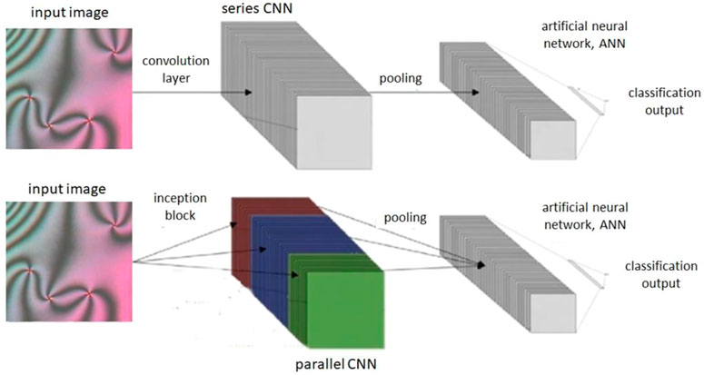
FIGURE 3. Diagram of a CNN with one convolution layer and an Inception model with one Inception block, each followed by a pooling layer and ANN. Feature map outputs for each layer’s filters are shown as stacks.
These hyperparameter choices for convolution layers are the number and size of filters that the layer applies to its input. Whilst CNNs have layers in series, Inception models have convolution layers in parallel (Szegedy et al., 2014). These have a different number of filters and/or filter sizes each, as shown in Figure 3. For example, by including parallel layers with different choices of filter size, the model complexity can be increased. This also reduces the need to train models with different values for these hyperparameters (number of filters and filter size) for the convolution layers (Szegedy et al., 2014), in order to find the most generalizable model. Inception models have been shown to outperform series CNNs, however can be more computationally intensive (Szegedy et al., 2014).
3 Methodology
Phase transitions were recorded from natural sample preparations by polarized optical microscopy. POM was carried out with a Leica OPTIPOL polarizing microscope, equipped with a Linkam hot stage (LTSE350) with temperature controller (TP 94) and a UEye UI-3360CP-C-HQ video camera. Image acquisition was at a resolution of 2048 × 1088 pixels. Several different compounds were investigated, 5CB and 8CB (Gray et al., 1973) as achiral liquid crystals, and the homologues series Dn (n = 5–8) (Dierking et al., 1994) and Mn (n = 5, 6, 7, 9, and 10) (Schacht et al., 1995) as the chiral materials. All recorded videos had all of their frames extracted. These were then sorted into their different phases. The resulting dataset of all textures available for use had 43.423 textures obtained from 129 videos. These were collected for the phases Iso: 3133, N: 8120, N*: 19664, SmA: 2506, SmC: 5406, SmI: 1340, and SmF: 3254.
The final preprocessing step was to convert the extracted images from PNG format to JPEG. This was done to reduce the storage requirements of the images, with negligible loss in quality. Images were resized to 256 × 256 pixels to reduce computational demands of the models. Further, every image was converted to grayscale to allow the models to focus on the textures rather than color, which does not affect the LC phase. Google Colaboratory (For “Google Colaboratory” see, 2022), which offers 12 GB GPU RAM, was used to train all the models in this project. By reducing their storage requirements, images could be stored in memory. This allowed for faster model training times, with all models taking less than 2 h. Models were created using the Keras deep learning framework (For “Keras API” see, 2022).
For each targeted transition, the first step was to find the possible test videos for the transition. Next, a dataset of the phases involved in the transition needed to be made. Any images from the test videos were removed from the dataset so that the test videos remained unseen by the models. To create a balanced dataset, where all phases have a similar number of examples, the phase with the larger number of images had images removed. This is known as undersampling. One can show that it is not convenient to simply randomly remove images until the dataset is balanced. This allows for phases to be overrepresented by textures from any single video. To avoid this, images were removed from the most overrepresented videos for the phase that needed reducing. For example, if the phase that needed reducing had 1,000 images from one video and 30,000 from another, 1 in every 30 images from the overrepresented video would be kept in the dataset. With the dataset created, it was then randomly split into training and validation sets with an approximate 3:1 split, as is common practice in machine learning (Russell and Norvig, 2010). It was also made sure that images from the same video were not split among training and validation sets, so that the validation set images remained unseen.
With a dataset for the targeted transition created, deep learning models were trained for the classification of the images. Due to the number of hyperparameters that can be tuned in deep learning models, we focused on the number of layers of the models, and use of dropout and flipping augmentation (Dierking, Dominguez, Harbon, and Heaton). Flipping was chosen as it was the only augmentation technique, offered by Keras, which was compatible with the OpenCV library (For “Open CV” see, 2022) used for labelling test videos. Additionally, for all models trained, the optimizer was chosen to be the default Adam-Optimizer (Kingma et al., 2017), due to its efficient performance with little hyperparameter tuning (Kingma et al., 2017). Finally, all models were trained for 40 iterations through the training data, known as epochs, as this was enough for training to plateau or start overfitting.
All models were saved at their epoch of lowest validation loss. By repeating training for each model, the average validation accuracy of the saved models was calculated. The results of this optimization study, varying layers, inception blocks, dropout and augmentation are provided elsewhere (Dierking, Dominguez, Harbon, and Heaton). Here, the model with the highest average validation accuracy was selected to be applied to the test videos. This involved classifying the test videos frame-by-frame with the chosen model. By relating the known temperature range of a video and the constant heating or cooling rate to the number of frames in the video, each frame could be associated with its temperature. From this, graphs of phase prediction probability were plotted against temperature. The crossover of phase probabilities in these graphs indicated a detected transition and its related phase transition temperature.
4 Results and discussion
4.1 Transitions between the isotropic and nematic phases
At first, models for the binary classification between the Iso and N textures were trained. As Iso-N transitions are visually simple to identify, only series convolutional neural networks (CNN models) were trained for this task. The dataset used for training models to distinguish Iso and N textures consisted of 4,963 training images each for Iso and N, and 1,720 validation images each for Iso and N. To balance this dataset, 3,669 low brightness noise images were added to the Iso training set and 602 to the validation set. This was also done to avoid models misclassifying low brightness N textures, for example homeotropic boundary condition nematic phases, for Iso.
All models achieved an average validation accuracy above 90%. This was to be expected due to the simplicity of the classification task. The highest average accuracy model investigated was a CNN with four convolution layers and no regularization. This model achieved a validation accuracy of 99.9%.
There were six videos available, of the 5CB and 8CB liquid crystals, showing Iso-N transitions. The model chosen to be applied to these test videos identified all Iso-N transitions accurately. Figure 4 shows a typical test video result. From this graph, it was determined that the Iso-N transition occurred at (35.6 ± 0.1)°C. The error was taken to be the relative error of the hot stage used to heat the LC in the video. This transition temperature was consistent with a visual inspection of the video, as shown by the inclusion of frames from the video in Figure 4.
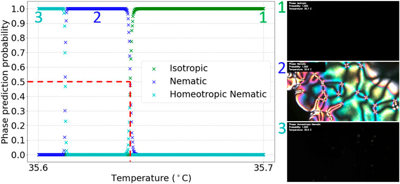
FIGURE 4. Graph of phase prediction probability against temperature for a labelled I-N transition test video. The vertical dashed line shows the identified transition temperature.
Figure 4 also demonstrates the use of this method for homeotropic N textures, which are visually indistinct from Iso textures, hence their name, pseudo-isotropic. Although the CNN cannot distinguish between Iso and homeotropic N images, by using the information that N had previously been predicted in the video, the algorithm was able to overwrite subsequent Iso predictions with homeotropic N predictions. This is suitable only for Iso-N transitions upon cooling, from Iso to N, and assumes no re-entrant behavior. For the latter to be predicted, one would need to label the training data accordingly.
4.2 Transitions between the isotropic and cholesteric phases
The split of images used to train CNN models for classifying between Iso and N* textures were 3308 training images and 1563 validation images for each of the Iso and N* phase. 2939 low brightness noise images were introduced into the isotropic training set and 1104 into the isotropic validation set, for the same reasons as explained above.
The same experimentation with series CNN models was done as with Iso-N classification in Section 4.1. Similarly, all models achieved a validation accuracy close to 100%. A model with three convolution layers, 0.5 dropout and flipping augmentation achieved 100% validation accuracy on all three repeats of training and was chosen to be used on the test videos. There were fifteen test videos showing Iso-N* transitions, including the D5 to D8 and M6 to M10 LCs. Overall, all test videos had their Iso-N* transition labelled consistently with visual inspection. Figure 5 depicts an example of a typical result with the transition temperature determined to (136.3 ± 0.1)°C.
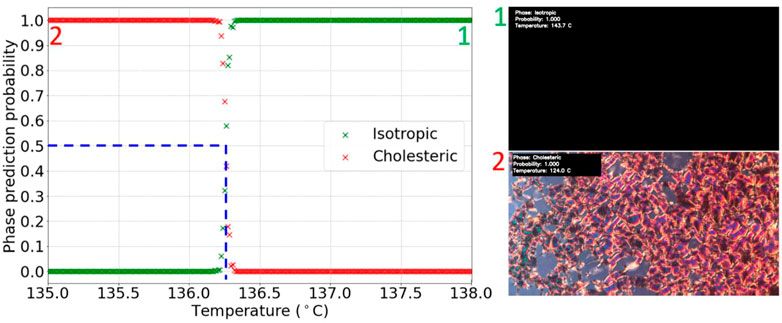
FIGURE 5. Graph of phase prediction probability against temperature for a labelled Iso-N* transition test video. The vertical dashed line shows the identified transition temperature.
The machine learning identified Iso-N* transition of compound D6 very well reproduces the experimentally determined temperature of 135.6°C (Dierking et al., 1994).
4.3 Transitions between the nematic and smectic a phases
As outlined above, the k-fold cross validation method can be more reproducible when using small datasets for classification tasks. Table 1 shows the training and validation splits for the five cross-validation datasets made for classifying between N and SmA textures.
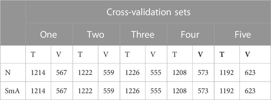
TABLE 1. Number of training (T) and validation (V) images in the N-SmA datasets.
Inception models are of higher capacity than CNNs and thus potentially more accurate for classifying between these phases, which can indeed look rather similar. Therefore, inception models were used here, also to demonstrate the variety of convolutional networks that may be used for the above datasets. Inception models with one and two inception blocks were trained for this task, with different regularization. Table 2 shows the average results of the models with the highest average validation accuracy for each of the five datasets. These models were chosen to be applied to the test transition videos. Errors given in these results come from half the range of results from three training repeats. Sets one, three and five achieved a lower accuracy than two and four. This shows how, when using deep learning techniques with a limited dataset, the specific choice of which images are in the training and validation sets can affect model performance. This is because the dataset does not contain a wide variety of the different textures that can be seen.
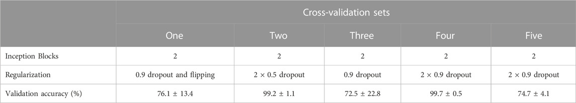
TABLE 2. Results for the highest validation accuracy models trained on each set of data.
There were five test videos for the N-SmA transition of 8CB. After applying the chosen models from each cross-validation set to the test videos, it was found that the set one and two models were unable to identify any transitions in the videos. The models from sets three, four and five accurately identified all test video transitions. When looking at the validation set textures for the models which were inaccurate on test videos, it was observed that most of the SmA textures were focal conics. These are visually distinct from the type of SmA textures in the test set videos. This further indicates the need to create a dataset with a wide variety of textures to train models which can generalize to many possible phase textures.
Figure 6 shows a typical test video result, using the model trained on set four. From the graph, the transition was determined to be at (33.4 ± 0.1)°C. The uncertainty was taken to be the approximate width of the region around which the phase prediction probabilities cross. This was considered to be consistent with the literature value of the N-SmA transition for the 8CB LC, 33.6°C (Struth et al., 2011), assuming an absolute temperature error of ±2°C due to different hot stages employed and other effects, such as rate of heating, causing a variation in transition temperature measurements.
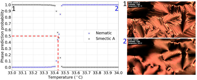
FIGURE 6. Graph of phase prediction probability against temperature for a labelled N-SmA transition test video. The vertical dashed line shows the identified transition temperature.
4.4 Transitions between the cholesteric and fluid smectic phases
For this classification task, there were six test videos showing examples of N*-fluid smectic transitions, specifically N*-SmC*. The dataset created for this task consisted of 4,226 training and 3,138 validation images for N*, and 3,854 training and 3,010 validation images for the fluid smectic phases. The fluid smectic textures were made up of SmA and SmC textures, with approximately an equal number of each in the training and validation sets. In making this dataset balanced, N* images had to be undersampled from approximately 18,000 to approximately 7,000, following the procedure as explained above.
The same type of analysis as for the achiral N-SmA transition in the previous section via Inception models was performed for this classification task. As expected, the results were similar, and the same model with two Inception blocks and two 0.9 dropout layers was chosen to be applied to the test videos. This model achieved 99.6% validation accuracy. Overall, all six test video transitions were accurately labelled, and Figure 7 shows a typical example of the chosen model’s labelling of the test videos.
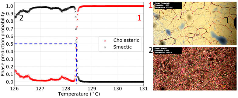
FIGURE 7. Graph of phase prediction probability against temperature for a labelled N*-SmC* transition test video. The vertical dashed line shows the identified transition temperature.
From Figure 7, the transition temperature was identified at (128.5 ± 0.1)°C, using the relative error of the hot stage. The literature value of the transition for this LC, M5, is 128.9°C (Schacht et al., 1995). The transition temperature is thus very well reproduced and any differences in absolute temperature values can easily be accounted for through the use of different hot stages in both investigations.
4.5 Transitions between the smectic A* and smectic C* phases
So far we have demonstrated the viability of machine learning to identify first order, discontinuous phase transitions. Here, we assess if it is also possible to characterize and classify a second order transition, namely the SmA* to SmC* transition. The training and validation split of images used is 1,088 training, 438 validation images for SmA* and 1,111 training and 422 validation images for SmC*. In creating this dataset, SmA* images needed to be undersampled, reducing the number of SmA* images from 2,383 to 1,526.
Due to the similarity in textures at a continuous transition, inception models were used for this classification. Most models tried, achieved an average validation accuracy close to 100%. Of these models, the one with a 0.5 dropout layer, a single Inception block and flipping augmentation had the highest average validation accuracy of 99.3% and was chosen to be applied to the test videos.
The result of applying the chosen model to the five possible SmA*-SmC* test videos was that only one transition was correctly identified. The graph and video screenshots for this video are shown in Figure 8. Taking the region of crossover between the phase prediction probabilities as the relative error, the transition was detected at (127.2 ± 0.4)°C. This was consistent with the literature value of 125.6°C for D8 (Dierking et al., 1994), again assuming an approximately ±2°C error in absolute temperature due to employing different hot stages. The value for the transition temperature was also consistent with visual inspection of the video. For the other test videos no transition was detected by machine learning algorithms. However, it should be noted that the transitions in these videos were visually much more subtle so these may have been too difficult for the model to distinguish, given the relatively small amount of training data. Overall, the model accurately identified a characteristic example of a SmA*-SmC* transition, however the inability to identify more subtle SmA*-SmC* texture change appearances implies that for continuous transitions much larger sets of training data need to be collected and most likely higher capacity machine learning algorithms need to be employed to found a more solid basis for the classification of second order transitions. Nevertheless, our investigation demonstrates proof of principle that this is indeed possible.
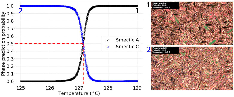
FIGURE 8. Graph of phase prediction probability against temperature for a labelled SmA*-SmC* transition test video. The vertical dashed line shows the identified transition temperature.
4.6 Transitions between the fluid smectic and hexatic phases
For this classification task, there were fourteen test videos showing examples of fluid smectic-hexatic transitions. As images from test videos cannot be used in training or validation, creating a single dataset with all fourteen videos in the test set was not possible. Therefore, two datasets were made for this classification task, with seven test videos held out for one dataset and the other seven held out for the other. This left enough images available for training and validation. The first and second dataset created for classifying between the fluid smectic and hexatic phases are shown in Table 3.
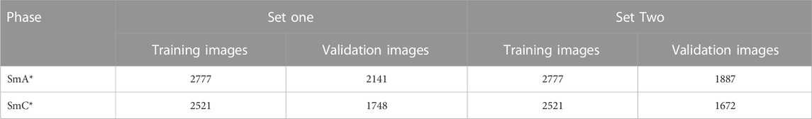
TABLE 3. Number of training and validation images in the fluid smectic-hexatic datasets.
Two different Inception model architectures were used for the classification, a model with one and another with two inception blocks. The latter constellation generally provided a higher accuracy. We also varied the regularization use, from applying no regularization, which led to overfitting, especially for the single block inception model. The use of two 0.99 dropout layers on the other hand led to underfitting. The highest average accuracy was achieved for a model with two Inception blocks and two 0.5 dropout layers, which was chosen for application to the test videos, and which achieved a validation accuracy of 91.7%. Similar results were achieved with the second dataset.
Overall, when applying the selected trained model to the test videos, one out of the thirteen was labelled accurately. This case is shown in Figure 9 and one can already see from the curves that the predictions are by far not as accurate as in the cases shown before, where the probabilities where basically either 0 or 1 with a precise changeover at the transition, while here the phase prediction probabilities change from 10% to 70% or vice versa, from 90% to 30%.
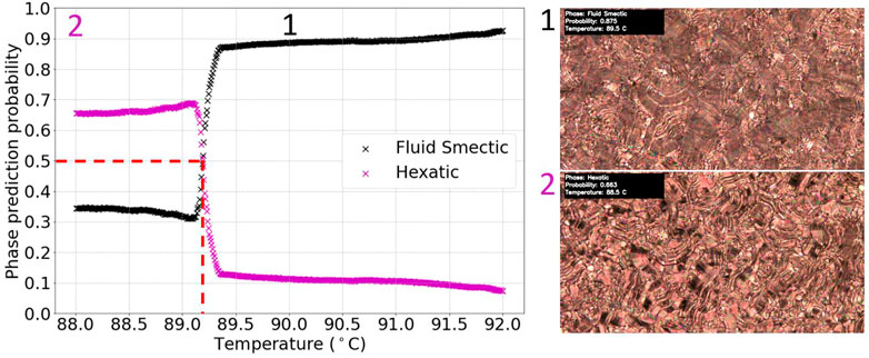
FIGURE 9. Graph of phase prediction probability against temperature for a labelled chiral fluid to hexatic (SmC*-SmI*) transition test video. The vertical dashed line shows the identified transition temperature. The figure shows the accurately labelled test video (in contrast to the incorrectly labelled ones further below in Figure 10).
From Figure 9, showing the accurately identified fluid smectic-hexatic transition test video, the transition was identified at (89.2 ± 0.4)°C, with the relative error taken as the approximate width of the overlap region between the phase prediction probabilities. This was consistent with visual inspection of the video and the literature value of the transition for D6, 90.5°C (Dierking et al., 1994), when accounting for factors which affect transition temperatures by a few degrees (different hot stages, cooling rate etc.). We note that although a large change in prediction probability is observed at the transition from fluid to hexatic smectic, an increasing order of the liquid crystal phase leads to a larger uncertainty in phase prediction. This is due to the fact that with increasing order when lowering the temperature, the actual changes in texture at transitions become more and more subtle, and phases are becoming less and less distinguishable by their textures. This is a further indication for the need to use more and larger training sets, as well as higher capacity models for prediction. The smaller the differences in the images which need to be categorized the more examples are needed for training and the more complex the employed models need to be.
More insight into the model’s performance can be gained by analyzing the inaccurately labelled test videos. With nine of the thirteen test videos, although inaccurately labelled, the model showed a sign of textural change indicated by a noticeable probability change at the transition. Figure 10 shows an example of one of these test videos. The fluid smectic-hexatic transition in this video occurred where the small probability change is seen in the graph, at approximately 91.2°C. A transition was then incorrectly identified at 97.0°C ± 2.0°C, because the helical structure of the fluid smectic phase changes considerably at the latter temperature, due to an unwinding which is interpreted by the algorithm as a phase change. It should be noted that this is specific to chiral phases, because in the achiral analogy of this transition no helical superstructures would be involved at all. The latter scenarios should be considerably easier to be classified.
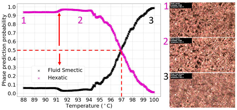
FIGURE 10. Graph of phase prediction probability against temperature for a labelled chiral fluid smectic- hexatic (SmC*-SmI*) transition test video. The vertical dashed line shows the incorrectly identified transition temperature, due to changes in the helical superstructure, while the arrow indicates the real transition.
The performance of the model on the video in Figure 10 can be explained using the included video frames. These show that the change of texture at the transition was more subtle than the change seen as the helical structure changes in the SmC* phase. A large proportion of the fluid smectic dataset contained textures with this helical characteristic. Therefore, the trained model recognizes the pattern changes as a phase transition, because it is the most obvious textural difference between the fluid smectic and hexatic phases. In an attempt to train a model which could correctly identify the subtle change that occurs at the transition, all textures with the helical pattern were removed from the dataset. However, using this dataset, models never achieved significantly above 50% validation accuracy. This was due to too few training sets for learning the subtle differences in the textures. To improve a model’s generalizability for this transition, more images should be collected, with a priority for obtaining textures that occur just after the transition, without the helix variation.
4.7 Transitions between the smectic I* and smectic F* phases
The final transition targeted in our investigation was that between the two chiral hexatic phases, SmI* and SmF*. Again, the dataset was split into two, one with five test videos left out (set 1), and one with four test videos left out (set 2). These are shown in Table 4.
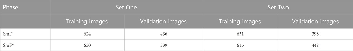
TABLE 4. Number of training and validation images for the SmI*-SmF* datasets.
The initial employment of inception models only achieved approximately 50% validation accuracy, which implies that the classification was basically random guesses. This was likely due to the small number of images available. Series CNNs were also trained to see if lower capacity algorithms could reach a better accuracy. Unfortunately, the models trained did not return a validation accuracy larger than 50% for dataset 1. However, with set 2, a model with four CNN layers, flipping augmentation and 0.5 dropout, achieved an 78.5% average validation accuracy, and was chosen to be applied to the test videos for set 2 of the dataset.
For set 1 of the datasets, all transitions in the five videos were missed while for the model chosen from set 2, three of the four test videos had their transitions missed. For the other test video, the results are shown in Figure 11. This transition was found to be at (81.7 ± 0.5)°C. The relative error on this measurement was taken to be the approximate width of the region around which the phase prediction probabilities crossed. Again, this was determined to be consistent with the literature value for D8, of 83.7°C (Dierking et al., 1994). It was also consistent with visual inspection of the video, as indicated by the frames included in Figure 11. Nevertheless, the phase prediction probabilities are again clearly different from 0 to 1, due to the uncertainties in the prediction.
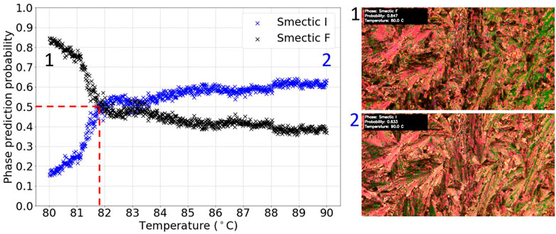
FIGURE 11. Graph of phase prediction probability against temperature for a labelled SmI*-SmF* transition test video. The vertical dashed line shows the identified transition temperature.
Overall, a generalizable model for identifying transitions between SmI* and SmF* phases was not achieved, most likely due to the rather limited dataset. Although further analysis with varying choices of training and validation sets as well as model architecture could be done, the collection of more data would be the most effective way of achieving such a generalized model, due to the subtlety of the transition and the variety of textures possible. Nevertheless, the accurately identified SmI*-SmF* transition provides proof-of-principle for the possibility of deep learning to identify this transition.
5 Conclusion
The results of this investigation show that deep learning models are capable to be trained for the identification of liquid crystal phase transitions from video recordings of experimental polarizing optical microscopy. It was clearly demonstrated that simple transitions of achiral as well as chiral systems, such as I-N, I-N*, N-SmA and N*-SmC* transitions, could accurately be identified in all unseen test videos via deep learning. Phase transition temperatures can accurately be identified, provided a suitable temperature calibration is done for the investigated movies. When targeting more subtle LC transitions, such as the 2nd order transition SmA*-SmC*, the fluid smectic-hexatic (SmC*-SmI*), and the inter hexatic SmI*-SmF* transition, proof-of-concept examples of accurately labelled transitions were demonstrated. Explanations for any inaccurately identified transitions, such as the variation of a helical superstructure in fluid smectic C* textures, were provided. These would be eliminated if only achiral materials were studied. Generalizable models capable of accurately identifying a wider range of these transitions was beyond the scope of this study due to the limited variety of texture examples available. Yet, without the limitations of datasets and computing power, there is no principal reason why one could not automate the identification of phase sequences of novel compounds by deep learning with suitable neural network algorithms of sufficient capacity.
Data availability statement
The data analyzed in this study is subject to the following licenses/restrictions: Video file of large size. Requests to access these datasets should be directed to ID, ingo.dierking@manchester.ac.uk.
Author contributions
ID conceived and directed the study, and contributed through discussions and writing of the manuscript. JD carried out the computer analysis of the texture videos, JH and JH contributed through discussions of the algorithms employed.
Conflict of interest
The authors declare that the research was conducted in the absence of any commercial or financial relationships that could be construed as a potential conflict of interest.
Publisher’s note
All claims expressed in this article are solely those of the authors and do not necessarily represent those of their affiliated organizations, or those of the publisher, the editors and the reviewers. Any product that may be evaluated in this article, or claim that may be made by its manufacturer, is not guaranteed or endorsed by the publisher.
References
Berrar, D. (2019). “Cross-validation,” in Encyclopedia of bioinformatics and computational biology. Editors S. Ranganathan, M. Gribskov, K. Nakai, and C. Schönbach (Oxford, England: Oxford Academic Press), 542–545. https://www.sciencedirect.com/science/article/pii/B978012809633820349X (Accessed 6 Nov. 2022).
Dierking, I., Dominguez, J., Harbon, J., and Heaton, J. In preparation to be submitted to Liq. Cryst.
Dierking, I., Giesselmann, F., Kusserow, J., and Zugenmaier, P. (1994). Properties of higher-ordered ferroelectric liquid crystal phases of a homologous series. Liq. Cryst. 17, 243–261. doi:10.1080/02678299408036564
Emeršič, Z., Štepec, D., Štruc, V., and Peer, P., “Training convolutional neural networks with limited training data for ear recognition in the wild,” in Proceedings of the 2017 12th IEEE International Conference on Automatic Face Gesture Recognition (FG 2017), 2017, pp. 987–994.
For Google Colaboratory, ” see (2022). https://colab.research.google.com/ (Accessed 6 Nov).
For Keras Api, ” see (2022). https://keras.io/ (Accessed 6 Nov).
For Open Cv, ” see (2022). https://opencv.org/ (Accessed 6 Nov).
Gray, G. W., Harrison, K. J., and Nash, J. A. (1973). New family of nematic liquid crystals for displays. Electron. Lett. 9, 130. doi:10.1049/el:19730096
Khadem, S. A., and Rey, A. D. (2021). Nucleation and growth of cholesteric collagen tactoids: A time-series statistical analysis based on integration of direct numerical simulation (dns) and long short-term memory recurrent neural network (LSTM-RNN). J. Colloid Interf. Sci. 582, 859–873. doi:10.1016/j.jcis.2020.08.052
Kingma, D. P., Ba, J., and Adam, (2017). A method for stochastic optimization. https://arxiv.org/abs/1412.6980 (last accessed 8 Nov. 2022.
LeCun, Y., Bengio, Y., and Hinton, G. (2015). Deep learning. Deep learning”, Nat. 521, 436–444. doi:10.1038/nature14539
Lecun, Y., Bottou, L., Bengio, Y., and Haffner, P. (1998). Gradient-based learning applied to document recognition. Proc. IEEE 86 (11), 2278–2324. doi:10.1109/5.726791
Lever, J., Krzywinski, M., and Altman, N. (2016). Model selection and overfitting. Nat. Methods 13, 703–704. doi:10.1038/nmeth.3968
Minor, E. N., Howard, S. D., Green, A. A. S., Glaser, M. A., Park, C. S., and Clark, N. A. (2020). End-to-end machine learning for experimental physics: Using simulated data to train a neural network for object detection in video microscopy. Soft Matter 16, 1751–1759. doi:10.1039/c9sm01979k
Russell, S., and Norvig, P. (2010). Artificial intelligence: A modern approach. 3rd ed. Upper Saddle River, NJ, USA: Pearson.
Schacht, J., Dierking, I., Giesselmann, F., Mohr, K., Zaschke, H., Kuczynski, W., et al. (1995). Mesomorphic properties of a homologous series of chiral liquid crystals containing the α-chloroester group. Liq. Cryst. 19, 151–157. doi:10.1080/02678299508031964
Sigaki, H. Y. D., Lenzi, E. K., Zola, R. S., Perc, M., and Ribeiro, H. V. (2020). Learning physical properties of liquid crystals with deep convolutional neural networks. Sci. Rep. 10, 7664. doi:10.1038/s41598-020-63662-9
Struth, B., Hyun, K., Kats, E., Meins, T., Walther, M., Wilhelm, M., et al. (2011). Observation of new states of liquid crystal 8cb under nonlinear shear conditions as observed via a novel and unique rheology/small-angle x-ray scattering combination. Langmuir 27, 2880–2887. doi:10.1021/la103786w
Szegedy, C, Liu, W, Jia, Y, and Sermanet, P, Reed, S, et al. (2014). Going deeper with convolutions”. CoRR, 4842. abs/1409 http://arxiv.org/abs/1409.4842 (last accessed 6 Nov. 2022.
Keywords: liquid crystal, machine learning, phase transition, deep learning, artificial neural networks
Citation: Dierking I, Dominguez J, Harbon J and Heaton J (2023) Deep learning techniques for the localization and classification of liquid crystal phase transitions. Front. Soft. Matter 3:1114551. doi: 10.3389/frsfm.2023.1114551
Received: 02 December 2022; Accepted: 20 January 2023;
Published: 03 February 2023.
Edited by:
Yanlei Yu, Fudan University, ChinaReviewed by:
Alejandro D Rey, McGill University, CanadaRalf Stannarius, Otto von Guericke University Magdeburg, Germany
Copyright © 2023 Dierking, Dominguez, Harbon and Heaton. This is an open-access article distributed under the terms of the Creative Commons Attribution License (CC BY). The use, distribution or reproduction in other forums is permitted, provided the original author(s) and the copyright owner(s) are credited and that the original publication in this journal is cited, in accordance with accepted academic practice. No use, distribution or reproduction is permitted which does not comply with these terms.
*Correspondence: Ingo Dierking, aW5nby5kaWVya2luZ0BtYW5jaGVzdGVyLmFjLnVr