Detection of forest disturbance across California using deep-learning on PlanetScope imagery

California forests have recently experienced record breaking wildfires and tree mortality from droughts, However, there is inadequate monitoring, and limited data to inform policies and management strategies across the state. Although forest surveys and satellite observations of forest cover changes exist at medium to coarse resolutions (30–500 m) annually, they remain less effective in mapping small disturbances of forest patches (<5 m) occurring multiple times a year. We introduce a novel method of tracking California forest cover using a supervised U-Net deep learning architecture and PlanetScope’s Visual dataset which provides 3-band RGB (Red, Green, and Blue) mosaicked imagery. We created labels of forest and non-forest to train the U-Net model to map tree cover based on a semi-unsupervised classification method. We then detected changes of tree cover and disturbance with the U-Net model, achieving an overall accuracy of 98.97% over training data set, and 95.5% over an independent validation dataset, obtaining a precision of 82%, and a recall of 74%. With the predicted tree cover mask, we created wall to wall monthly tree cover maps over California at 4.77 m resolution for 2020, 2021, and 2022. These maps were then aggregated in a post-processing step to develop annual maps of disturbance, while accounting for the time of disturbance and other confounding factors such as topography, phenological and snow cover variability. We compared our high-resolution disturbance maps with wildfire GIS survey data from CALFIRE, and satellite-based forest cover changes and achieved an F-1 score of 54% and 88% respectively. The results suggest that high-resolution maps capture variability of forest disturbance and fire that wildfire surveys and medium resolution satellite products cannot. From 2020 to 2021, California maintained 30,923.5 sq km of forest while 5,994.9 sq km were disturbed. The highest observed forest loss rate was located at the Sierra Nevada mountains at 21.4% of the forested area being disturbed between 2020 and 2021. Our findings highlight the strong potential of deep learning and high-resolution RGB optical imagery for mapping complex forest ecosystems and their changes across California, as well as the application of these techniques on a national to global scale.

1 Introduction

Climate change introduces increased risk of severe droughts in California and, consequently, extreme wildfires (Diffenbaugh et al., 2015). From 2011 to 2016, California experienced severe drought conditions and in 2020 had a record breaking wildfire season (McEvoy et al., 2020; Keeley and Syphard, 2021). In normal climate conditions, these forests play a major role in sequestering carbon and remain a robust carbon sink of atmospheric carbon of about 6–10 MT CO2e (Holland et al., 2019; Hudiburg et al., 2019; Walters et al., 2023). However, disturbance of live trees from drought mortality and wildfire significantly impact forest carbon sequestration capacity and California’s state-wide emission reduction policies. Forests also play an important role in the region’s economy, where management for timber extraction moved 135,351.9 m³ and $139,145,423.86 worth of cut timber in the 2020 fiscal year (Forest Products Cut and Sold from the National Forests and Grasslands, 2024). However, the capability to map trees statewide with a scale suitable for local applications is a crucial yet underexplored tool for effectively managing natural resources (Knight et al., 2022).

Forest disturbances in California have become increasingly critical in recent years as wildfires grow more frequent and intense (Wang et al., 2022). From 2000 to 2020, California lost approximately 226,000 ha contributing a 3.6% decrease in total forested area while maintaining 10.8 Mha of stable forest (Hansen, et al., 2013). Forest loss and disturbance in California is driven primarily by wildfires which are exacerbated by drought conditions, specifically increased temperatures and reduced precipitation (Wang et al., 2022). The risk of drought in California is also likely to increase as average global temperatures rise, making monitoring of tree cover and forest loss a crucial aspect for local conservation efforts and accuracy of global climate models (Littell et al., 2016). Fires in the last 5 years have moved beyond usual ranges of variation, destroying entire stands of trees and complicating fire risk management strategies (Cova et al., 2023). While wildfires pose a less controllable threat to forests, this challenge is compounded by historical logging practices, which have resulted in a 50% decline in large trees from the 1930s to the early 2000s (McIntyre, et al., 2015). Hence, mapping tree cover and evaluating changes resulting from disturbances are crucial pieces of information for conserving and managing these forests, ensuring their continued function as carbon sinks. There have been efforts in the past to map forest cover and changes at varying spatial and temporal resolutions (Hansen et al., 2002; Friedl et al., 2022). Most studies rely on Landsat (30 m) time series data to detect changes of forest cover (Hansen et al., 2013; Potapov et al., 2020). Higher resolution tree cover mapping from Sentinel-1 Synthetic aperture radar (SAR) data and Sentinel-2 optical imagery have improved the mapping unit to 10 m (Ottosen et al., 2020; Zhao, et al., 2022). However, the majority of these techniques are either applied globally, or have not been used to map statewide tree cover across California. Here, we use optical imagery from the PlanetScope constellation of CubeSats at 4.77 m spatial resolutions with daily revisits. The high fidelity in spatial and temporal resolutions significantly improve the availability of cloud free images across the state, allowing detection of forest disturbance at the time of occurrence and at the tree level. However, working with the PlanetScope imagery may have several disadvantages including: (i) lack of radiometric and atmospheric calibration of imagery, making image classification and time series analysis with conventional tools difficult, (ii) impacts of variations in illumination and viewing angles, causing difficulty in comparing images for detecting changes, and (iii) the large volume of data available in different shapes and sizes, making the data analytic computation costly. Additionally, the diverse forest landscapes of California, spanning from Chaparral to Redwoods, present unique challenges due to varying phenology, snow cover dynamics, and distribution across complex terrains. These limitations can be circumvented by using AI and cloud computing optimization techniques. Application of convolutional neural networks (CNNs) allow for the segmentation of tree cover at an unprecedented accuracy when coupled with high resolution satellite imagery from PlanetScope (Wagner et al., 2023a; Liu et al., 2023).

Specifically, the U-Net model (Ronneberger et al., 2015) has been widely applied to map a variety of forest processes such as forest types based on WorldView-3 and Sentinel-2 satellite data (Wagner et al., 2019; Wagner, 2021), as well as tree cover, deforestation and forest degradation in the tropics using Planet NICFI data (Wagner et al., 2023b; Dalagnol et al., 2023). These techniques require large-scale mosaics of very high-resolution image tiles for implementation of AI and development of regional or statewide maps (Kattenborn et al., 2020). The use of PlanetScope monthly basemap mosaics in the visual spectrum (R, G, and B bands) provided by Planet Labs at 4.77 m resolution could facilitate large-scale applications of imagery. By careful training of RGB imagery as input data, deep learning models have the capability of learning complex patterns and detect forest loss accurately over varied landscapes (Han and Sanchez-Azofeifa, 2022).

In this study, we aimed to achieve high-resolution classification of forest cover across California by leveraging a combination of 4.77-m resolution monthly mosaic images from PlanetScope, referred to as basemaps, and employing a deep learning U-Net model for tree cover segmentation. Our study yielded novel results in several key areas:

(i) Demonstrating the deep U-Net architecture’s capability to rapidly and accurately generate annual high-resolution forest cover maps at 4.77-m resolution.

(ii) Quantifying state-wide and regional annual changes in forest cover from 2020 to 2022.

(iii) Validating our results through comparisons with independently estimated tree cover from airborne LiDAR data, forest loss databases across California, and conducting comparisons with previous forest loss datasets.

2 Materials and methods

2.1 Study site

Our study site covers the entire state boundary of California, United States (Figure 1). This study region represents 423,971 km². The environment of California is a biodiversity hotspot (California Floristic Province) containing shrubby forests like the coastal sage scrub and chaparral, large coniferous forests, deserts, and urban regions (Myers et al., 2000). California’s mediterranean climate can be broken down to three distinct microclimates. First, the coastal range of California and the western Sierra Nevada mountain range are characterized by cool summers and cool winters with precipitation falling in the winter. Second, regions directly on the coast have a similar climate but often with fog in the summer which brings moisture to the area. Finally, the San Joaquin Valley and inland Southern California have hot summers and cool winters more typical of a desert climate (California Department of Fish and Game, 2003).

Figure 1

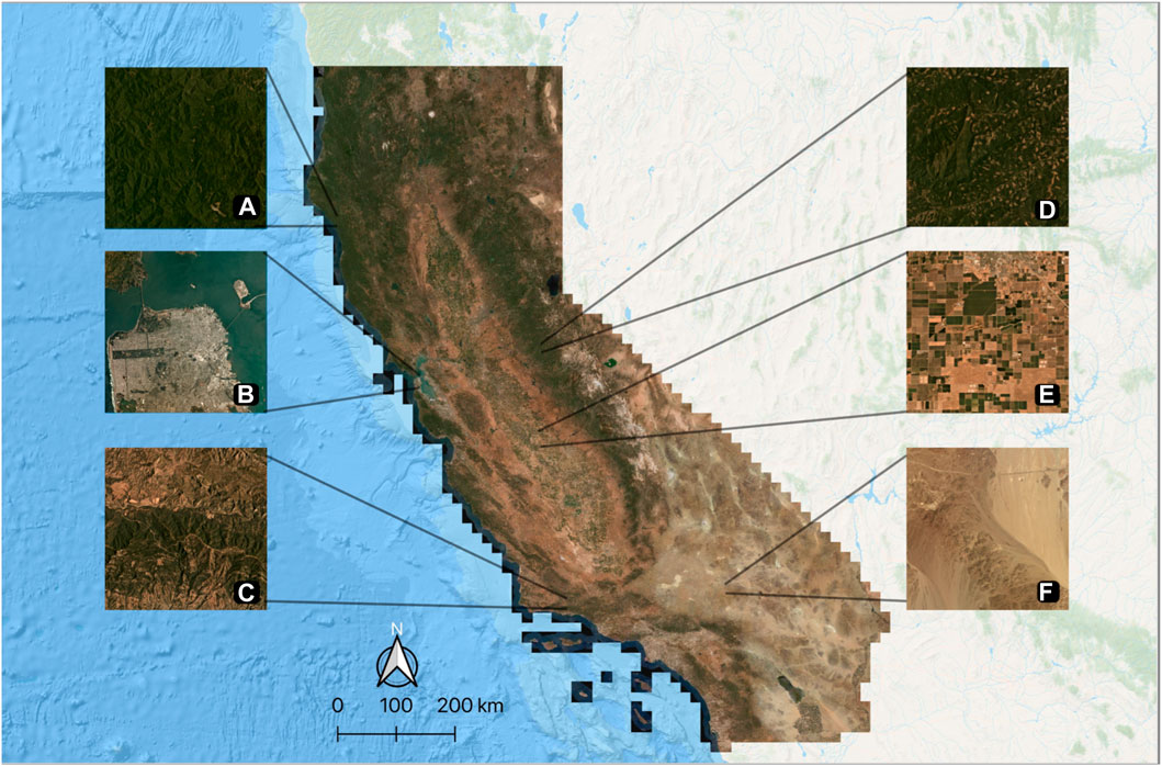
Figure 1. Study area at the state of California, United States. Different land types and regions are highlighted: (A) Dense evergreen forest, (B) Urban development (San Francisco Bay Area), (C) Chaparral, (D) Evergreen forest with lake and logging, (E) Agricultural land, (F) Desert. Background shows true color composite from PlanetScope RGB basemap.

2.2 PlanetScope satellite images

To estimate forest cover over the state of California, we obtained monthly mosaics of PlanetScope satellite images at 4.77 m spatial resolution from January 2020 to December 2022 with red (0.650–0.682 µm), green (0.547–0.585 µm), blue (0.464–0.517 µm) downloaded using the Planet API (Planet Team, 2017). These data are organized in 1,866 tiles of 20 km × 20 km (4,096 × 4,096 pixels) covering the entirety of California, United States (Figure 1). All images were in digital numbers (8 bits, 0 to 255 range). No preprocessing was performed in the imagery.

2.3 Airborne LiDAR data

To validate our forest cover map, we compared our results to airborne LiDAR canopy height models (CHM) data that were acquired from the United States Geological Survey (USGS) and National Ecological Observatory Network (NEON). This dataset is constituted of discrete-return LiDAR data from flight lines of 10 km long by 10 km wide distributed over California. The LiDAR dataset was acquired during 2018–2020 using the Optech Gemini and Riegl LMS-Q780 laser scanning systems at an average flight altitude of 1,000 m. Multiple LiDAR returns were recorded with a point density of 64 points per m². Initially, the point cloud LAS files were obtained over 11 NEON sites: YosemiteNP, UpperSouthAmerican\_Eldorado, SantaCruzCounty, SantaClaraCounty, NoCal, LassenNP, Fresno, CarrHirzDeltaFires, TEAK, SOAP, and SJER (Supplementary Figure S1). The LiDAR point clouds were processed into digital terrain models (DTM) and canopy height models (CHM) with 1 × 1 m cell size following procedures described in Wagner, et al. (2023a). The median of the data were aggregated at the resolution of the PlanetScope data (4.77 m). From the total 8113.8 km² of forest covered by 9188 canopy height tiles, we randomly selected 1,000 tiles to be used as our reference data which covered 895 km². These canopy height model tiles are used to validate our forest cover map as discussed in section 2.8.

2.4 Neural network architecture

The segmentation of forest cover was created using a classical U-net model (Figure 2). To train this model, we first selected 120 randomly sampled tiles across the study area, and created training labels of 256 × 256 pixels using the k-texture self segmentation model (Wagner et al., 2022). Next, these labeled training data were fed into the U-Net model which returns a pixel-wise probability of forest cover in a given input image. The model inputs for training were 3-bands (RGB) made up of 256 × 256 pixels and the output was a mask of one band and 256 × 256 pixels containing 1 (forest cover, pixel probability≥0.5 or 0 (non-forest, probability <0.5). The model was coded in R language with RStudio interface to Keras and TensorFlow 2.8 (Abadi, et al., 2016). The procedures are described in detail in the next subsections.

Figure 2

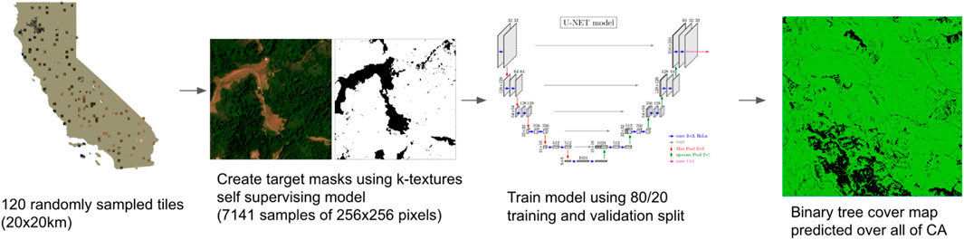
Figure 2. Diagram of the sampling and training process. Beginning with 120 randomly selected tiles, we create 7,141 image patch samples of 256 × 256 pixels using the K-textures self-supervised algorithm then fed into the U-Net architecture to create binary forest cover maps.

2.5 Label production and training

The model training followed an iterative active learning process of producing labels, training the U-Net model, evaluating results for inconsistencies, adding more training data and re-training the model, etc. First, initial training labels of forest cover were produced by randomly selecting Planetscope images over California for each monthly mosaic date from June 2020 to May 2022. We randomly select spatially and temporally in order to have images for all the seasons and distributed across different environments of California. Then, we performed self-segmentation with 7 classes using the k-textures model (Wagner et al., 2022) over the selected images. The k-textures is a deep learning-based algorithm which provides self-supervised segmentation of a 4-band image for k number of classes and is designed to ease the production of training labels for satellite image segmentation. After self-segmentation, we inspected the results to define which classes belonged to forest and non-forest classes. After verifying the k-texture results on the 120 images, the training dataset consisted of 3930 training samples of 256 × 256 pixels extracted from 23 images where the forest segmentation was deemed accurate according to visual interpretation. Small forest mask errors were manually corrected. The training dataset masks had two classes: forest (1) and non-forest (0), which contained agriculture, urban area, water surface, and bare ground.

Second, a U-Net model was trained to map tree cover using the training dataset. The model was then applied to predict the forest cover over the 1,866 image tiles in California for the date of June 2020. The results were visually inspected and identified areas with inconsistencies such as not correctly finding some forest types or returning false positives over non-forest areas. Two more iterations of active learning were performed. In our second iteration, we added 21 more images to increase the robustness of the algorithm, specifically over bodies of water and mixed forests and shrublands. In our final iteration, we added 69 images that included burnt regions and images with haze or light cloud cover. Images with thick clouds and heavy haze were removed while images with thin clouds and light haze were manually selected to train the model. Keeping only thin clouds and light haze allows the model to learn which forest images are recognizable to the human eye and which are not.

The final training dataset consisted of 7,141 image patches of 256 × 256 pixels and their associated labeled masks for the final U-net model. A total of 3,524 image patches contained forest and non-forest and 3,617 only non-forest. Of the total image patches, 80% (5,713) were used for training and 20% (1,428) for model validation and choosing the final set of weights to be applied for prediction of forest cover for the rest of California.

We employed a standard stochastic gradient descent optimization technique for network training. The loss function was formulated as the sum of the binary cross-entropy and Dice coefficient-related loss of the predicted masks. Finally, we used the Adam optimizer with a learning rate of 0.0001. Model performance was assessed using accuracy which measures frequency with which the prediction matches the observed value. The network was trained for 25,000 epochs with a batch size of 256 images and the model with the best weighted accuracy was kept for prediction (epoch 22,794 and training/validation accuracy of 98.97% and 95.02%, respectively, and training/validation loss of 0.0141 and 0.0874, respectively). The training of the model took approximately 12 h using a g5.4xlarge EC2 instance (GPU is Nvidia A10G Tensor Core with 24gb VRAM) on Amazon Web Services (AWS). During training, each image patch went through a data augmentation process that consisted of random vertical and horizontal flips (Chollet et al., 2022). No additional data augmentation was necessary due to the natural data augmentation provided by different atmospheric conditions and illumination due the different dates of the sampling images (Wagner et al., 2022).

2.6 Prediction

For the prediction of forest cover over California at each date, the borders of the full image tiles (4096 × 4096 pixels) were mirrored creating an additional 256 pixel border around it, thus having 4,608 × 4,608 pixels at the end. This was done to avoid edge artifacts during prediction. Mirroring the edges to avoid artifacts can produce marginally lower quality predictions at the edge but no noticeable difference was seen. Prediction of forest cover was made on the entire image and cropped to the original tile size of 4,096 × 4,096 pixels. Forest class pixels are defined as having a prediction value greater than or equal to 0.5 otherwise the pixel is classified as non-forest. For model training and inference we use Amazon Web Services EC2 instances which provide cloud-based GPU computation. The prediction of forest cover for one Planet tile took approximately 9 s using a g5.4xlarge EC2. We predicted over the 1,866 tiles of California and 36 monthly image mosaics from January 2020 to December 2022.

2.7 Annual forest cover and change maps

The production of annual forest cover and change maps considered a few steps and many challenges associated with the varied vegetation, terrain and climate of California. First, monthly basemap images show varying degrees of differential shading and changes in landscape due to seasonality. In the northern hemisphere, basemap images tend to have higher differential shading due to high azimuth angle of the sun resulting in shaded regions on northern aspect slopes that can be falsely predicted as forested areas. Second, high elevation regions (>1000 m) may have snow cover during the winter which our model invariably predicts as non-forest due to abnormally high reflectance values. Therefore, to create annual forest cover composites from monthly imagery for 2020, 2021 and 2022, we developed a temporal filter that takes the majority value of a given pixel over two time frames, all 12 months or 7 summer months (April to October), depending on elevation and slope aspect. In our filter, if a pixel had an elevation greater than 1,000 m or a northern aspect (>300 or <60°) then we determine the forest cover state by taking the sum of pixel values between the summer months and attributing a “Forested” value (in this case a value of 1) in pixels that had a sum greater than or equal to 4, and “Non-Forested” (0) for pixels with a sum less than 4. For a pixel outside of these elevation or aspect parameters, the threshold value for the sum of all 12 months was set to greater than or equal to 7 months. Elevation data from NASA’s Shuttle Radar Topography Mission (SRTM) was used to determine which pixels were above 1,000 m elevation and the aspect (Farr, et al., 2007).

Forest change maps were created by following the trajectory of pixels based on the three annual maps (2020, 2021, and 2022) and creating a map with the following classes: stable forest, stable non-forest, forest loss and forest gain from 2020 to 2022 (Figure 3).

Figure 3

Figure 3. Workflow diagram for the creation of annual tree cover and change maps. We begin by creating a stack of monthly forest cover predictions for each tile and adding elevation and aspect data to the stack. The stack is then sent to the annual composite filter where a majority filter is applied either to the mid-year months or the entire year depending on elevation and aspect of the pixel. The trajectory of pixels in annual composites (forest/non-forest) are then tracked from 2020 to 2022 resulting in four classes: stable non-forest, stable forest, forest loss, and forest gain.

2.8 Validation and comparison with existing datasets

Independent validation of the monthly predictions was performed by comparing forest cover map created by our mapping approach in 2019 to forest heights from 2019 LiDAR CHMs. Because the CHM dataset was created for 2019, we created tree cover maps for 2019 in the interest of temporal consistency between our validation data and tree cover predictions. The data were split into pixels predicted as forest and non-forest from our forest cover map and then the median height of the CHM within each pixel was calculated to understand the distribution of height in the forest and non-forest categories.

The location of forest management (logging) and fires in California were obtained from the CALFIRE database to validate the predicted forest losses from our model (Fire Perimeters CAL FIRE, 2024). According to the California State Geoportal website, “over-generalization, particularly with large old fires, may show unburned ‘islands’ within the final perimeter as burned. Users of the fire perimeter database must exercise caution in application of the data,” (Fire Perimeters CAL FIRE, 2024). The CALFIRE dataset is the most up to date data on fire and logging available in California but presents limitations such as areas which may be shown as undisturbed forest within the disturbed polygons perimeter, or disturbed forests outside of the perimeter of existing polygons. We evaluate our model against the logging and fire perimeters considering the F1-score metric.

To compare our results to a previous existent dataset, we obtained the Global Forest Change (GFC) global tree loss year product at 30 m resolution from 2020 to 2022. For our analysis we use the 2021 GFC year loss product in comparison to forest losses found by our model from 2020 to 2022. We choose these years of comparison because of time lag in loss recognition between both our model and the GFC model. Because forest fires in California most often occur in the second half of the year, from late July to October, our method of creating annual composites has a tendency to pick a burned region as disturbed in the second composited year. We chose the 2021 years loss data because it is the center of our period of interest. If a region is burned according to the year loss data we want to know if our model identified the region as deforested between 2020 and 2022. Our data resolution was downscaled to the GFC resolution of 30 m by assigning 1 (forest loss), if >70% of pixels were predicted as forest loss, or 0 (no forest loss), if≤70% of pixels were predicted as forest loss. We compared the similarity of our results to the GFC dataset by calculating their weighted intersection.

$WeightIntersection=\frac{\cap {\left(LossPixel{s}_{unet,i},LossPixel{s}_{GFC,i}\right)}^2}{LossPixel{s}_{GFC,i}{\sum }_{i=1}^n\left(\cap \left(LossPixel{s}_{unet,i},LossPixel{s}_{GFC,i}\right)\right)}$

where ${LossPixels}_{\mathit{Ours},\mathit{i}}$ and ${LossPixels}_{\mathit{GFC},\mathit{i}}$ represents the number of pixels in a tile i, that were predicted as forest loss in our time of interest, and n represents the total number of tiles in California (1866).

3 Results

3.1 Training validation

Our U-net model has a training accuracy of 98.97%, validation accuracy of 95.5%, a precision of 82%, a recall of 74%, and an F-1 score of 0.778. This validation is conducted by comparing our predicted values to our visually assigned labels from the semi-supervised training dataset. The training accuracy is conducted over the same dataset on which the U-net model is trained, representing 80% of all training data. The validation accuracy is conducted over the 20% of the training dataset that is not included in the training of the U-net to ensure independence.

3.2 Validation of individual predictions using airborne LiDAR data

We used an independent validation technique comparing our individual monthly predictions to a LiDAR canopy height model for the month of June 2019. Setting the height threshold at 5 m, according to the International Geosphere-Biosphere Program (IGBP) definition for forest cover, we saw an overall accuracy of 77.77%, an 82% precision of pixels predicted as forest cover and 74% precision of pixels predicted as non-forest cover. When the two forest cover categories were compared, we found the differences of the mean heights to be 29.871 m with a 95% confidence interval of 29.858 m and 29.884 m and a p-value <2.2*10 ^ -16 (Figure 4). The first, second, and third quartile values of forested pixels were 10 m, 31 m, and 55 m and the non-forested pixels were 0 m, 0 m, and 6 m (Figure 5). Figure 6 shows a visual example of the segmentation of forest cover and non-forest cover achieved by our model.

Figure 4

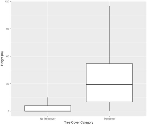
Figure 4. Box plot showing the average, quartile and range of height values over non-tree covered and tree covered pixels in individual predictions.

Figure 5

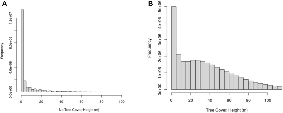
Figure 5. Image (A) shows the distribution of CHM height values over pixels predicted as no tree cover while image (B) shows the distribution of height values over pixels predicted as tree cover.

Figure 6

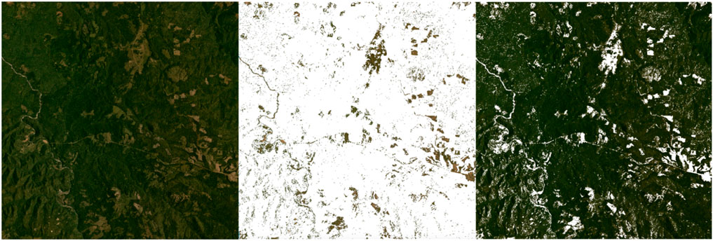
Figure 6. 20 × 20 km tile in Northern California from June 2020 side by side with the prediction from our U-net model. Left: RGB image. Middle: Forest masked in white. Right: Background masked in white.

3.3 Validation of annual forest cover using airborne LiDAR data

We applied the same validation method to our annual tree cover composite and found nearly the same results as our individual predictions. The difference of the mean heights of tree cover and non-treecover pixels for the annual composite validation was 29.819 m with a confidence interval of 29.815 and 29.820 and a p value < 0.001 (Figure 7). The annual composite had a 74% precision of pixels predicted as non-forest cover (Figure 8A) and 82% precision for pixels predicted as forest cover (Figure 8B). Using the same 5 m tree height definition for forest, our annual composite had an accuracy of 77.30%.

Figure 7

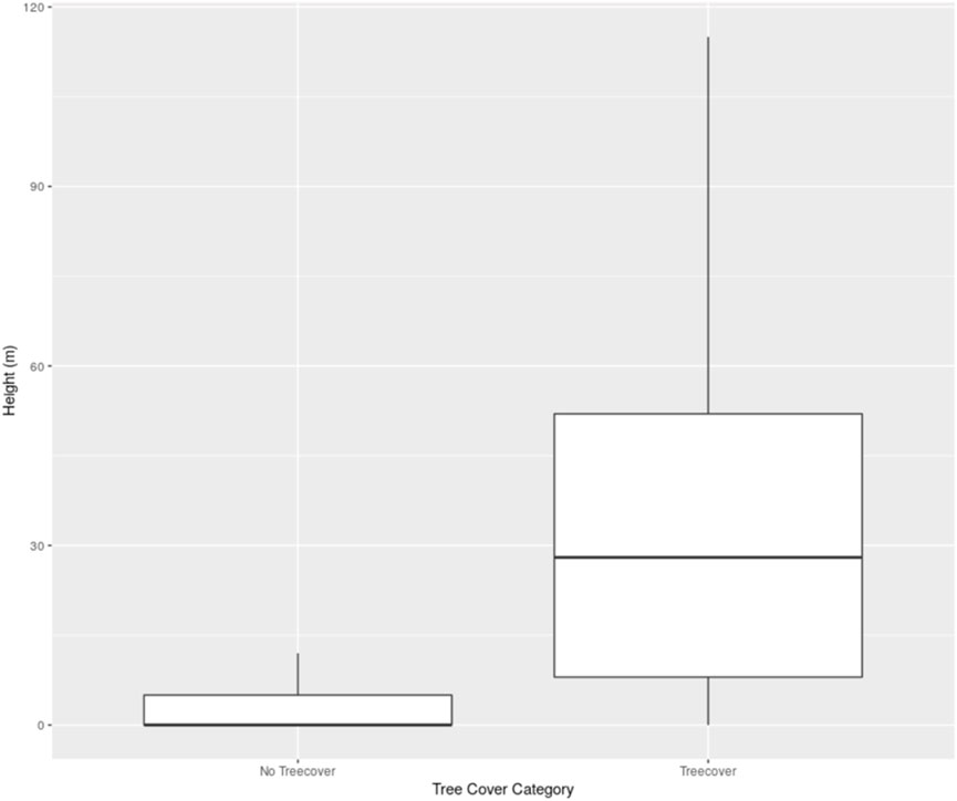
Figure 7. Box plot showing the average, quartile and range of height values over non-tree covered and tree covered pixels in the annual composite for 2019.

Figure 8

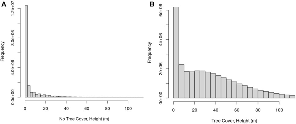
Figure 8. Image (A) shows the distribution of CHM height values over pixels attributed to no tree cover in the annual composite while image (B) shows the distribution of height values over pixels attributed to tree cover.

3.4 Validation of forest loss regions

Our F1 score, calculated as overlap between what our model classified as loss and known regions of forest loss (CALFIRE), is 54.5%. It is important to note that in many logging regions the area is not completely deforested and our model is capable of picking up very small patches or even single trees. Similarly, fire shapefiles show the furthest extent of fire in a region but this does not equate to every tree inside the shapefile being disturbed. For example, in the Creek Fire region, Figure 9, we see that the shapefile outlines the maximum extent of the fire but does not necessarily describe the intensity of the fire inside as our F1 score in this region is 71.8%. In comparison to the area mapped by the perimeter as burned for the Creek Fire of 3273.61 km² by CALFIRE, our map shows 888.15 km² of forest loss. By inspecting the overlaid fire perimeter on top of our map (Figure 9), our map shows that part of the areas (984.01 km² or 30.01% of total fire area) were in fact non-forest before the fire occurred. Similar examples can be found in logging concession areas (Figure 10) where we see some remaining trees within the boundary of the CALFIRE perimeter.

Figure 9

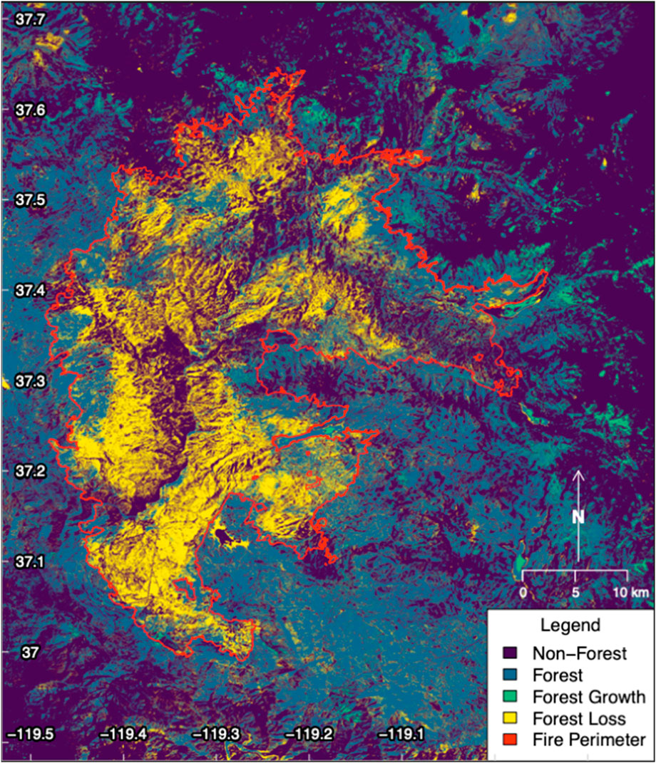
Figure 9. Creek Fire, near Shaver Lake, California, burned in September and October of 2020 and was one of California’s largest fires. Red regions show areas of forest loss between 2020 and 2021, green shows areas of maintained forest, black are areas of non-forest, and yellow are regions of forest gain.

Figure 10

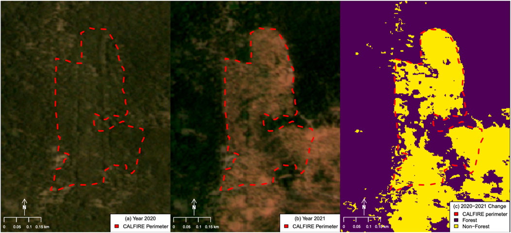
Figure 10. Image (A) shows regions of forest loss due to logging. Image (B) shows the shapefile of the logging allotment from the state of California. Image (C) shows our map of forest loss from 2020 to 2021 created from our predictions.

3.5 Forest cover and change in California

California’s forest cover in 2020, 2021, and 2022, was calculated at 17,042,653.7, 14,283,221.0, and 16,547,832.1 ha, respectively (Figure 11). This represents 40.1%, 33.7%, and 39.0% of the total area of California (Table 1). We see a net decline in the years of 2020–2021 of 2,756,432.7 ha and 2,264,611.1 ha of net growth in forest cover from 2021 to 2022. This loss from 2020 to 2021 is primarily driven by forest fires of both natural and anthropogenic causes such as arson, fallen power cables, or lightning strikes. 2020 accounted for 5 of the top 10 largest known fires in California. The percent loss of forest from 2020 to 2021 is 16.17%.

Figure 11

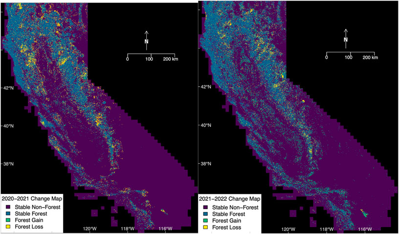
Figure 11. Side by side change maps from 2020 to 2021 (left) and 2021–2022 (right). Black: no tree cover, purple: tree cover, blue: tree cover gain, yellow: tree cover loss.

Table 1

Table 1. Total forest cover and percentage land cover estimates from 2020 to 2022.

The total forest loss area from 2021 to 2022 is 1,559,581.31 ha 2021 to 2022 also saw a significant increase in the amount of “growth” regions (non-forested areas that became forested) when compared to 2020 to 2021. Many of these areas were in previous fire regions which were disturbed, but perhaps not completely deforested. This type of forest loss can be picked up in the first time period as “forest loss” but then considered “forest gain” in the next year.

Most forested areas in California are located along the various mountain ranges in the state, namely, Sierra Nevada, Cascade, and Coastal Ranges. Within the Sierra Nevada range, 5,138,237.51, 4,231,106.54, and 3,975,634.39 ha had forest cover in 2020, 2021, and 2022, respectively (Table 2). From 2020 to 2021, the Sierra Nevada region saw a total disturbed area of 907,130.97 ha and total forested area of 4,231,106.54 ha. From 2021 to 2022, 674,461.08 ha were disturbed in the Sierra Nevadas while 3,975,634.39 ha remained forest between the 2 years. The ratio of forest loss to stable forested area, which we will refer to as the “forest loss ratio”, over 2020 to 2021 is 0.214 and for 2021 to 2022 is 0.170. The marked difference in the ratio of forest loss to stable forested area over the two time periods is driven by massive fires in California in 2020. The Creek fire alone, which occurred in September of 2020, contributed approximately 153,738.052 ha of forest loss in the Sierra Nevada range.

Table 2

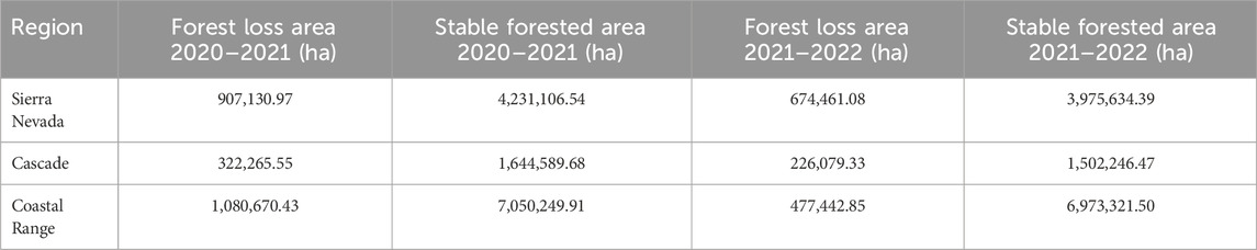
Table 2. Regional tree cover and forest loss over 3 forest regions of California: Sierra Nevada Mountain Range, Cascade Mountains, and the Coastal Range.

In the Cascade range of Northern California, we see a total area of 322,265.55 ha and 226,079.33 ha of forest loss and maintained 1,644,589.68 ha and 1,502,246.47 ha in 2020–2021 and 2021 to 2022, respectively. Like the Sierra Nevadas, there is significantly less forest loss in the 2021 to 2022 period than the 2020 to 2021 period. The forest loss ratio from 2020 to 2021 is 0.196, similar to the forest loss ratio seen in this period in the Sierra Nevadas. From 2021 to 2020 we observe a forest loss ratio of 0.150. From these ratios, we can conclude that the Sierras and Cascade mountains had similar levels of forest loss when compared to each other.

Finally, in the Coastal Range, which spans much of the western border of the state, we see a total disturbed area of 1,080,670.43 ha and 477,442.85 ha from 2020 to 2021 and 2021 to 2022, respectively. The area of remaining forest in these two time periods are 7,050,249.91 ha and 6,973,321.50 ha. The forest loss ratio in 2020–2021 is 0.153 and in 2021–2022 is 0.068.

3.6 Comparison to GFC product

We compare our data to the GFC product first by a direct comparison of forested area in California and secondly by calculating the weighted intersection between our forest change product and the GFC year loss product. In 2020, 2021, and 2022, GFC estimates that there were 9.2, 8.9, and 8.4 Mha of natural forest in California. Our model found on average about 55% more forested area in California from 2020 than GFC in 2020. Our product in 2020, 2021, and 2022, estimates 17,042,653.7, 14,283,221.0, and 16,547,832.1 ha of forest cover, respectively. Our forest loss results show strong overlap with the GFC year loss product. Figure 12 shows the change map for the Creek Fire region from our model (Figure 12a) from 2020 to 2021 and the forest loss over the same period from GFC. Using the 2021 GFC year loss data as a reference, our forest loss prediction has a weighted intersection of 88.0%.

Figure 12

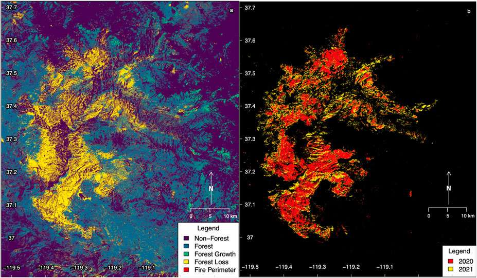
Figure 12. Comparison of disturbed area from 2020 to 2021 in Creek Fire region. Image (A) shows our predicted forest loss area, while image (B) shows the various years of forest loss in 2020 and 2021 from the GFC model.

4 Discussion

4.1 Deep learning approach to mapping forest cover in California

In this study, for the first time we map forest cover and forest change of California at high resolution (4.77 m) using PlanetScope imagery and a deep learning approach. From 2020 to 2022, California had a net loss of 494821.6 ha of forest cover. Our findings show that the forest cover of California varied from 44.7% in 2020, to 33.7% in 2021, and 39.0% in 2022. Using PlanetScope’s monthly visual datasets (RGB bands) at 4.77 m resolution, our U-Net model achieved a validation accuracy of 95.02% in the our validation dataset. The deep CNN model uses the RGB values of the pixel of interest as well as the structure of surrounding pixels to determine whether a pixel is forested or non-forested. This allows the model to accurately assess the state of each pixel over the 36 month period. One of the novelties of this study is the application of such a model over a complex environment of various land cover types, such as California, as well as capturing the spatial and spectral patterns across a wide temporal range using only RGB mosaics. Previous studies have applied similar methods using the Planet NICFI analytic data which includes the NIR band to map dense tropical forests in the Brazilian state of Mato Grosso (Wagner et al., 2023a). Additionally, Planet analytics data sets in conjunction with U-Net deep learning models and LiDAR data have been used to create tree height and biomass models over Europe (Liu et al., 2023). Limited preprocessing of the images and faster training data collection using the K-textures (Wagner, et al., 2022) model allow for fast and accurate estimates of forest cover over diverse ecosystems. This methodology coupled with large, cloud-based processing servers (such as Amazon web services or Google cloud services) could help to make forest cover estimates on a national, continental, or even global scale.

4.2 Annual change from 2020 to 2022

Approximately 2,756,432.7 ha of California’s forests were disturbed from 2020 to 2021 and a net forest loss of 494821.6 ha from 2020 to 2022. We expect this large swing from net forest loss in 2020–2021 and regrowth from 2021 to 2022 has two causes. The first is genuine forest loss from natural and anthropogenic causes such as forest fires, logging (USFS, 2020 Annual Cut and Sold Report), and forest management. According to CALFIRE, approximately 1.7 million hectares of forest were burned in 2020 across 8648 wildfires (CALFIRE). The extra 1.056 million hectares of forest loss likely comes in part from data outside of CALFIRE dataset such as smaller-scale logging, and agricultural regions. Edge regions of forests and trees in cities are more prone to error in our model because there is less forest context for the model to work with. However, within a given perimeter of logging or fire from CALFIRE our model provides a more accurate estimate of forest loss than the total contained area because of its ability to distinguish burned and unburned regions within the perimeter (Figure 10). The second reason for this large discrepancy is regreening of regions of forest burned in the prior year. Immediately after a wildfire, short and understory vegetation are completely burned as well as some of the leaves of the canopy trees, but tree mortality may not always occur (Hood, et al., 2018). This allows for a regreening effect in the following year in which the model picks up the texture and color of the forest as a “regrowth”. Finally, any errors that exist in either dataset can contribute to the discrepancy as well.

On a regional scale, we see that from 2020 to 2021 the Sierra Nevadas had the highest forest loss ratio, followed by the Cascades, then the Coastal Ranges. There are three possible causes for this. First, because of their proximity to the Pacific Ocean, forests in the coastal range can remain cooler during late summer when the fire season is at its peak and additional moisture from the ocean may help quell fire severity. Second, the southern Coastal range is dominated by Chaparral forests which are less appealing for loggers compared to the tall conifers found in the Sierra Nevada and Cascade ranges. Thirdly, also in the presence of Chaparral regions, the model has a harder time distinguishing between forested and non-forested areas which can contribute to inaccuracies in spotting disturbed areas between years. Using tree height to classify forest and non-forest may improve accuracy in difficult regions like Chaparral (Liu et al., 2023). However, the IGBP definition of forest height at 5 m may exclude regions of Chaparral that have vegetation but are lower than the 5 m threshold. This could lead to higher error for this biome compared to other in California. Years with especially large fires and total burn areas are also associated with higher frequency of lightning storms that ignite the forest (Miller et al., 2012). Large lightning induced fires in Northern California, like the August complex and SCU lightning complex, contributed to the record breaking fire season. Higher temperatures that increase evapotranspiration and increased risk of severe drought as climate change develops leaves California at high risk for widespread wildfires caused by large lightning storms.

4.3 Comparison to GFC data

Our model found on average 55% more forested area from 2020 to 2022 compared to GFC tree cover estimates in 2010. The discrepancy in forested area estimates is likely due to differences in spatial resolution. Our map at 4.77 m is capable of picking up more areas of scattered forest that may not be detected by the 30 m resolution of Landsat. Tree growth in California from 2010 to 2022 is a less likely contributor as California suffered drought conditions from 2011 to 2017 which lead to tree mortality, especially in larger individuals (Bennett et al., 2015).

We found a strong overlap between our model and the GFC year loss from 2021 with a weighted intersection of 88%. The remaining 12% difference is primarily due to regions inside forest fire perimeters that the GFC model picked up as disturbed but our model did not. There are two possible sources of error. First, because the GFC model has 30 m resolution, it may miss unburned “islands” of forest that occur within a designated burned perimeter. Our model is capable of properly distinguishing these regions as undisturbed because of its higher spatial resolution which results in a non-intersection over some pixels. Second, our model may erroneously label regions that were destroyed in fires as forest due to remaining shading artifacts. Differential shading causes certain regions of an image to appear especially dark, and can be mislabeled as forest when contrasted with surrounding burned areas that have higher reflectance. Given the high intersection value, our model is capable of finding most of the same regions of forest loss as the GFC year loss product as well as small scale forest losses outside of the scope of the GFC product.

4.4 Quality of PlanetScope basemaps data

The 3-band (RGB) data from PlanetScope Basemaps provided enough data to achieve high accuracy on mapping the forest cover of California. However, it provides less spectral information than other analytic datasets which include the NIR band, such as the Planet NICFI for the tropical regions, or other coarser resolution satellite data such as from Sentinel-2 or Landsat. However, the Planet basemaps are already offered in a mosaicked format which allows users to easily input the data into deep learning models with no pre-processing. This tradeoff can possibly create less accurate results compared to a model that uses 4-band data that includes the near-infrared (NIR) band commonly used in remote sensing of vegetation. The inspection of this difference in quality between 3 and 4-band data with a deep CNN is an interesting area of focus for future research. In addition to the lower spectral information, the 3-band Planet mosaics also contain some haze and clouds which impair our model’s ability to accurately infer forest cover over these regions. This issue was mostly resolved by training the model over regions with light haze and clouds where the forest was still visible to a human observer as well as our annual filtering process.

4.5 Topography and seasonality of data

A limitation for our model comes from the topography and seasonality of California. Topology of California can create issues of differential shading in the images which, in darker areas, the model often classifies as forested because of the darker characteristics of the pixels. Even a human cannot distinguish if the given area is a shadow or a forest in a shadow. This effect may occur more frequently only in regions with sparse or low canopy vegetation, such as the chaparral region of southern California (Syphard, et al., 2019). Seasonality in California also presents the challenge of snow cover in mountainous, high-altitude regions like the Sierra Nevada range. In our study, we already took precautions to minimize these effects in the post-processing step by using different rules considering elevation and slope data to account for these effects. However, we acknowledge these areas are still prone to errors. For the expansion of this methodology to the contiguous United States (CONUS), deciduousness of the trees in the eastern half of the CONUS will need to be accounted for by expanding the training data to contain such seasonal variations in tree morphology.

4.6 Impact

The combined use of the semi-supervised k-textures model to produce labeled training samples over California with the U-Net architecture allowed for a rapid and accurate prediction of monthly forest cover over California from 2020 to 2022. Because of its speed, ease of use, and the adaptability of the U-Net architecture, this methodology can be applied to assess forest cover and forest change from jurisdictional to continental scales. Our model was able to create novel high resolution wall to wall forest cover maps over California that capture both large scale forests and smaller clumps of trees outside of forests. This is a first step towards the implementation of inter-annual monitoring of forest cover in California, which can contribute to improving estimates of carbon losses and gains in the region, inform restoration groups and policymakers of regions potentially more vulnerable to wildfires, which is important given that managed forests are part of the region’s economy. The method and maps presented here can be continually improved in future versions. Future work will include the use of the Planet visual basemaps to predict forest height by using lidar training data. Training our model to use the NIR band found in the PlanetScope analytic data could help further improve accuracy due to its relationship with vegetation structure and potentially reduce errors caused by differential shading or seasonally phenology. Additionally, separating non-forest classes into water and agricultural classes could improve our model accuracy by giving direct examples of these classes. This could reduce the error of predicting agriculture and water regions as natural forest. Given California has a wide variety of complex vegetation from coast to desert and mountains we expect this model has the potential to be further tested and applied to the continental United States creating a comprehensive, high-resolution forest cover and forest change map.

5 Conclusion

Our study produced monthly wall to wall forest cover maps of California using a deep convolutional neural network and Planet’s visual basemap imagery from 2020 to 2022. Our individual predictions showed promising results with a validation accuracy of 95.02% and an independent validation of 77.77% at 4.77 m spatial resolution when forests are defined with a height greater than 5 m based on airborne LiDAR data. We then filtered the monthly maps to create annual forest cover maps which had an overall accuracy of 82%. The difference between annual forest cover maps created the change maps from 2020 to 2021 and 2021 to 2022 with a validation accuracy of 54.5% using CALFire logging shapefiles. From 2020 to 2021, California saw a net reduction of forest cover by 2,756,432.7 ha while from 2021 to 2022 we saw a recovery of forest cover by 2,264,611.1 ha. This study shows the viability of deep convolutional neural networks in predicting forest cover in highly diverse biomes, like California, using only 3-band RGB datasets. Due to the versatility and speed of the model, these methods can likely also be upscaled to the national or continental levels. The creation of such accurate, high resolution forest cover maps at a wide range of scales can help track and monitor forest changes across various biomes.

Data availability statement

The raw data supporting the conclusion of this article will be made available by the authors, without undue reservation.

Author contributions

GC: Writing–original draft, Writing–review and editing, Conceptualization, Data curation, Formal Analysis, Investigation, Methodology, Software, Validation, Visualization. FW: Writing–original draft, Writing–review and editing, Conceptualization, Data curation, Formal Analysis, Investigation, Methodology, Software, Validation, Visualization. RD: Conceptualization, Data curation, Investigation, Methodology, Validation, Writing–review and editing. SR: Data curation, Formal Analysis, Investigation, Methodology, Software, Validation, Writing–original draft, Writing–review and editing. AR: Data curation, Writing–original draft, Writing–review and editing. SS: Conceptualization, Data curation, Formal Analysis, Funding acquisition, Investigation, Methodology, Project administration, Resources, Supervision, Writing–review and editing.

Funding

The author(s) declare that no financial support was received for the research, authorship, and/or publication of this article. This research received no external funding.

Acknowledgments

The authors are grateful to the Grantham and High Tide Foundations for their generous gift to UCLA and grants to CTrees for bringing new science and technology to solve environmental problems. This work was partially conducted at the Jet Propulsion Laboratory, California Institute of Technology under a contract (80NM0018F0590) the National Aeronautics and Space Administration (NASA).

Conflict of interest

The authors declare that the research was conducted in the absence of any commercial or financial relationships that could be construed as a potential conflict of interest.

Publisher’s note

All claims expressed in this article are solely those of the authors and do not necessarily represent those of their affiliated organizations, or those of the publisher, the editors and the reviewers. Any product that may be evaluated in this article, or claim that may be made by its manufacturer, is not guaranteed or endorsed by the publisher.

Supplementary material

The Supplementary Material for this article can be found online at: https://www.frontiersin.org/articles/10.3389/frsen.2024.1409400/full#supplementary-material

References

Abadi, M., Barham, P., Chen, J., Chen, Z., Davis, A., Dean, J., et al. (2016) TensorFlow: a system for large-scale machine learning.

Google Scholar

Bennett, A. C., McDowell, N. G., Allen, C. D., and Anderson-Teixeira, K. J. (2015). Larger trees suffer most during drought in forests worldwide. Nat. Plants 1, 15139–15145. doi:10.1038/nplants.2015.139

PubMed Abstract | CrossRef Full Text | Google Scholar

California Department of Fish and Game (2003) Atlas of the biodiversity of California. California, USA: 2nd Edition.

Google Scholar

Chollet, F., Kalinowski, T., and Allaire, J. J. (2022) Deep learning with R. Shelter Island, NY: Manning.

Google Scholar

Cova, G., Kane, V. R., Prichard, S., North, M., and Cansler, C. A. (2023). The outsized role of California’s largest wildfires in changing forest burn patterns and coarsening ecosystem scale. For. Ecol. Manag. 528, 120620. doi:10.1016/j.foreco.2022.120620

CrossRef Full Text | Google Scholar

Dalagnol, R., Wagner, F. H., Galvão, L. S., Braga, D., Osborn, F., Sagang, L. B., et al. (2023). Mapping tropical forest degradation with deep learning and Planet NICFI data. Remote Sens. Environ. 298, 113798. doi:10.1016/j.rse.2023.113798

CrossRef Full Text | Google Scholar

Diffenbaugh, N. S., Swain, D. L., and Touma, D. (2015). Anthropogenic warming has increased drought risk in California. Proc. Natl. Acad. Sci. 112, 3931–3936. doi:10.1073/pnas.1422385112

PubMed Abstract | CrossRef Full Text | Google Scholar

Farr, T. G., Rosen, P. A., Caro, E., Crippen, R., Duren, R., Hensley, S., et al. (2007). The Shuttle radar topography mission. Rev. Geophys. 45. doi:10.1029/2005RG000183

CrossRef Full Text | Google Scholar

Fire Perimeters CAL FIRE (2024). Fire. Available at: https://www.fire.ca.gov/what-we-do/fire-resource-assessment-program/fire-perimeters (Accessed March 29, 2024).

Google Scholar

Forest Products Cut and Sold from the National Forests and Grasslands (2024). Usda. Available at: https://www.fs.usda.gov/forestmanagement/products/cut-sold/index.shtml (Accessed March 29, 2024).

Google Scholar

Friedl, M. A., Woodcock, C. E., Olofsson, P., Zhu, Z., Loveland, T., Stanimirova, R., et al. (2022). Medium spatial resolution mapping of global land cover and land cover change across multiple Decades from Landsat. Remote Sens. 3. doi:10.3389/frsen.2022.894571

CrossRef Full Text | Google Scholar

Han, T., and Sanchez-Azofeifa, G. A. (2022). A deep learning time series approach for Leaf and wood classification from Terrestrial LiDAR point clouds. Remote Sens. 14, 3157. doi:10.3390/rs14133157

CrossRef Full Text | Google Scholar

Hansen, M. C., DeFries, R. S., Townshend, J. R. G., Sohlberg, R., Dimiceli, C., and Carroll, M. (2002). Towards an operational MODIS continuous field of percent tree cover algorithm: examples using AVHRR and MODIS data. Remote Sens. Environ. Moderate Resolut. Imaging Spectroradiom. MODIS a new generation Land Surf. Monit. 83, 303–319. doi:10.1016/S0034-4257(02)00079-2

CrossRef Full Text | Google Scholar

Hansen, M. C., Potapov, P. V., Moore, R., Hancher, M., Turubanova, S. A., Tyukavina, A., et al. (2013). High-resolution global maps of 21st-century forest cover change. Science 342, 850–853. doi:10.1126/science.1244693

PubMed Abstract | CrossRef Full Text | Google Scholar

Holland, T. G., Stewart, W., and Potts, M. D. (2019). Source or Sink? A comparison of Landfire- and FIA-based estimates of change in aboveground live tree carbon in California’s forests. Environ. Res. Lett. 14, 074008. doi:10.1088/1748-9326/ab1aca

CrossRef Full Text | Google Scholar

Hood, S. M., Varner, J. M., Mantgem, P., and Cansler, C. A. (2018). Fire and tree death: understanding and improving modeling of fire-induced tree mortality. Environ. Res. Lett. 13, 113004. doi:10.1088/1748-9326/aae934

CrossRef Full Text | Google Scholar

Hudiburg, T. W., Law, B. E., Moomaw, W. R., Harmon, M. E., and Stenzel, J. E. (2019). Meeting GHG reduction targets requires accounting for all forest sector emissions. Environ. Res. Lett. 14, 095005. doi:10.1088/1748-9326/ab28bb

CrossRef Full Text | Google Scholar

Kattenborn, T., Eichel, J., Wiser, S., Burrows, L., Fassnacht, F. E., and Schmidtlein, S. (2020). Convolutional Neural Networks accurately predict cover fractions of plant species and communities in Unmanned Aerial Vehicle imagery. Remote Sens. Ecol. Conservation 6, 472–486. doi:10.1002/rse2.146

CrossRef Full Text | Google Scholar

Keeley, J. E., and Syphard, A. D. (2021). Large California wildfires: 2020 fires in historical context. Fire Ecol. 17, 22. doi:10.1186/s42408-021-00110-7

CrossRef Full Text | Google Scholar

Knight, C. A., Tompkins, R. E., Wang, J. A., York, R., Goulden, M. L., and Battles, J. J. (2022). Accurate tracking of forest activity key to multi-jurisdictional management goals: a case study in California. J. Environ. Manag. 302, 114083. doi:10.1016/j.jenvman.2021.114083

CrossRef Full Text | Google Scholar

Littell, J. S., Peterson, D. L., Riley, K. L., Liu, Y., and Luce, C. H. (2016). A review of the relationships between drought and forest fire in the United States. Glob. Change Biol. 22, 2353–2369. doi:10.1111/gcb.13275

PubMed Abstract | CrossRef Full Text | Google Scholar

Liu, S., Brandt, M., Nord-Larsen, T., Chave, J., Reiner, F., Lang, N., et al. (2023). The overlooked contribution of trees outside forests to tree cover and woody biomass across Europe. Sci. Adv. 9, eadh4097. doi:10.1126/sciadv.adh4097

PubMed Abstract | CrossRef Full Text | Google Scholar

McEvoy, D. J., Pierce, D. W., Kalansky, J. F., Cayan, D. R., and Abatzoglou, J. T. (2020). Projected changes in reference evapotranspiration in California and Nevada: implications for drought and Wildland fire Danger. Earth’s Future 8, e2020EF001736. doi:10.1029/2020EF001736

CrossRef Full Text | Google Scholar

McIntyre, P. J., Thorne, J. H., Dolanc, C. R., Flint, A. L., Flint, L. E., Kelly, M., et al. (2015). Twentieth-century shifts in forest structure in California: Denser forests, smaller trees, and increased dominance of oaks. Proc. Natl. Acad. Sci. 112, 1458–1463. doi:10.1073/pnas.1410186112

PubMed Abstract | CrossRef Full Text | Google Scholar

Miller, J. D., Skinner, C. N., Safford, H. D., Knapp, E. E., and Ramirez, C. M. (2012). Trends and causes of severity, size, and number of fires in northwestern California, USA. Ecol. Appl. 22, 184–203. doi:10.1890/10-2108.1

PubMed Abstract | CrossRef Full Text | Google Scholar

Myers, N., Mittermeier, R. A., Mittermeier, C. G., Fonseca, G., and Kent, J. (2000). Biodiversity hotspots for conservation priorities. Nature 403, 853–858. doi:10.1038/35002501

PubMed Abstract | CrossRef Full Text | Google Scholar

Ottosen, T. B., Petch, G., Hanson, M., and Skjøth, C. A. (2020). Tree cover mapping based on Sentinel-2 images demonstrate high thematic accuracy in Europe. Int. J. Appl. Earth Obs. Geoinf 84, 101947. doi:10.1016/j.jag.2019.101947

PubMed Abstract | CrossRef Full Text | Google Scholar

Planet Team (2017). “Planet application Program interface,” in Space for Life on Earth. Available at: https://api.planet.com (accessed on January 10, 2023).

Google Scholar

Potapov, P., Hansen, M. C., Kommareddy, I., Kommareddy, A., Turubanova, S., Pickens, A., et al. (2020). Landsat analysis Ready data for global land cover and land cover change mapping. Remote Sens. 12, 426. doi:10.3390/rs12030426

CrossRef Full Text | Google Scholar

Remote Sensing (2024). Free full-Text | Landsat analysis Ready data for global land cover and land cover change mapping. Available at: https://www.mdpi.com/2072-4292/12/3/426 (Accessed March 28, 24).

Google Scholar

Ronneberger, O., Fischer, P., and Brox, T. (2015) U-net: convolutional networks for Biomedical image segmentation. doi:10.48550/arXiv.1505.04597

CrossRef Full Text | Google Scholar

Syphard, A. D., Brennan, T. J., and Keeley, J. E. (2019). Extent and drivers of vegetation type conversion in Southern California chaparral. Ecosphere 10, e02796. doi:10.1002/ecs2.2796

CrossRef Full Text | Google Scholar

Wagner, F. H. (2021). The flowering of Atlantic forest Pleroma trees. Sci. Rep. 11, 20437. doi:10.1038/s41598-021-99304-x

PubMed Abstract | CrossRef Full Text | Google Scholar

Wagner, F. H., Dalagnol, R., Sánchez, A. H., Hirye, M. C. M., Favrichon, S., Lee, J. H., et al. (2022). K-textures, a self-supervised hard clustering deep learning algorithm for satellite image segmentation. Front. Environ. Sci. 10, 946729. doi:10.3389/fenvs.2022.946729

CrossRef Full Text | Google Scholar

Wagner, F. H., Dalagnol, R., Silva-Junior, C. H. L., Carter, G., Ritz, A. L., Hirye, M. C. M., et al. (2023a). Mapping tropical forest cover and deforestation with Planet NICFI satellite images and deep learning in Mato Grosso state (Brazil) from 2015 to 2021. Remote Sens. 15, 521. doi:10.3390/rs15020521

CrossRef Full Text | Google Scholar

Wagner, F. H., Roberts, S., Ritz, A. L., Carter, G., Dalagnol, R., Favrichon, S., et al. (2023b) Sub-meter tree height mapping of California using Aerial images and LiDAR-Informed U-net model. doi:10.48550/arXiv.2306.01936

CrossRef Full Text | Google Scholar

Wagner, F. H., Sanchez, A., Tarabalka, Y., Lotte, R. G., Ferreira, M. P., Aidar, M. P. M., et al. (2019). Using the U-net convolutional network to map forest types and disturbance in the Atlantic rainforest with very high resolution images. Remote Sens. Ecol. Conservation 5, 360–375. doi:10.1002/rse2.111

CrossRef Full Text | Google Scholar

Walters, B. F., Domke, G. M., Greenfield, E. J., Smith, J. E., and Ogle, S. M. (2023) Greenhouse gas emissions and removals from forest land, woodlands, and urban trees in the United States, 1990-2021: estimates and quantitative uncertainty for individual states, regional ownership groups, and National Forest System regions. doi:10.2737/RDS-2023-0020

CrossRef Full Text | Google Scholar

Wang, J. A., Randerson, J. T., Goulden, M. L., Knight, C. A., and Battles, J. J. (2022). Losses of tree cover in California driven by increasing fire disturbance and climate stress. AGU Adv. 3, e2021AV000654. doi:10.1029/2021AV000654

CrossRef Full Text | Google Scholar

Zhao, F., Sun, R., Zhong, L., Meng, R., Huang, C., Zeng, X., et al. (2022). Monthly mapping of forest harvesting using dense time series Sentinel-1 SAR imagery and deep learning. Remote Sens. Environ. 269, 112822. doi:10.1016/j.rse.2021.112822

CrossRef Full Text | Google Scholar