 Juliette Bernard1,2*
 Catherine Prigent1,3Carlos Jimenez1,3
 Frédéric Frappart4
 Cassandra Normandin4Pierre Zeiger5
 Yi Xi2
 Shushi Peng6
- 1LERMA, CNRS, Observatoire de Paris, Paris, France
- 2Laboratoire des Sciences du Climat et de l’Environnement (LSCE), Gif-sur-Yvette, France
- 3Estellus, Paris, France
- 4ISPA, UMR 1391 INRAE/Bordeaux Science Agro, Villenave-d’Ornon, France
- 5Institut des Géosciences de l’Environnement (IGE), Grenoble, France
- 6College of Urban and Environmental Sciences, Peking University, Beijing, China
Inland waters, especially wetlands, play a crucial role in biodiversity, water resources and climate, and contribute significantly to global methane emissions. This study investigates the seasonal and inter-annual variability of the 0.25° × 0.25° surface water extent (SWE) from the Global Inundation Extent from Multi-Satellites (GIEMS-2) extended to a 30-year time series (1992–2020). Comparison with MODIS-derived SWE, CYGNSS-derived SWE and the Global Lakes and Wetlands Database (GLWD) shows consistent spatial patterns globally and over 10 different basins, although there are discrepancies in extent, partly due to different resolutions of the initial satellite observations. Strong cross-correlation (
1 Introduction
Inland surface waters influence the ecological and climatic balance of our planet. Rivers and lakes play a role in the hydrological cycle as well as in human activities such as agriculture. Wetlands regulate freshwater, host rare and diverse fauna and flora, and store carbon in peatlands (Denny, 1994; Meli et al., 2014; Poulter et al., 2021). Moreover, these areas contribute significantly to global emissions of methane, a potent greenhouse gas (Torres-Alvarado et al., 2005; Saunois et al., 2020). Approximately one-third of the total methane emission is estimated to come from inland water systems, and these natural methane emissions represent the largest uncertainty in the global budget and a major contributor to its inter-annual variability (Wania et al., 2013; Saunois et al., 2020). For these reasons, the monitoring of surface waters at local and global scales over long time series is essential in the context of climate change, with these ecosystems particularly vulnerable to significant alterations (Papa and Frappart, 2021; Cretaux et al., 2023) and affected by floods and droughts of unprecedented magnitude (Kreibich et al., 2022).
The dynamics of surface waters can be simulated using hydrological models and observed from in situ measurements or from satellites. Models allow the study of periods or locations where few or no observations are available, and can provide projections into the future. However, these models have large uncertainties due to the challenges of understanding, representing, and parameterizing all the processes involved (Kraft et al., 2022). Relevant in situ and remote sensing observation data offer another approach to quantify key variables linked to the water cycle (Fernández-Prieto et al., 2012; Fassoni-Andrade et al., 2021). They are useful to evaluate or feed models using different integration approaches (Kraft et al., 2022).
Measurements of surface water extent rely exclusively on remote sensing data, as there are only a few in situ flood monitoring stations worldwide, and these are not capable of measuring flood extent. Different remote sensing techniques are commonly used to map Surface Water Extent (SWE) dynamics. They include the use of visible and near-infrared (NIR) images acquired at medium and high spatial resolution at a daily (Moderate Resolution Imaging Spectroradiometer, MODIS) to bi-monthly (Landsat missions) temporal sampling, providing observation over several decades (Pekel et al., 2016; Huang et al., 2018). Visible and NIR observations are severely impacted by clouds and vegetation, preventing the continuous estimation of SWE dynamically on a global scale. Microwave observations are particularly relevant for wetland studies because they can penetrate clouds and vegetation better. Passive microwave satellite observations from Special Sensor Microwave/Imager (SSM/I) and Special Sensor Microwave Imager Sounder (SSMIS) instruments provide twice-daily observation long time series (from the 90s) at low spatial resolution (from 69 km × 43 km at 19 GHz to 15 km × 13 km at 85 GHz). SWE detection using passive microwaves is limited by snow, ocean contamination, and confusion with desert signatures (Prigent et al., 2001). Surface water are also observed using active microwave sensors, with synthetic aperture radar (SAR) providing very high resolution data (down to 1 m) (Shen et al., 2019). However, SAR-based SWE are mostly regional or local, as it is difficult to retrieve water surfaces coherently on a global scale. In addition, the time resolution was poor before the launch of Sentinel-1 A and B in 2014 and 2016 enabling a 6-day revisit. Finally, L-band spaceborne GNSS reflectometry (GNSS-R) observations from the CYGNSS mission provides data at ∼ 1 km × 6 km resolution with a 7 h mean revisit time on a 25 km × 25 km pixel (Ruf et al., 2016). However, the actual coverage period is short (2016-present), and the spatial coverage ranges only from 40°S to 40°N.
To overcome the limitations of a single type of observations, the combination of multiple satellite measurements has been proposed to estimate surface water extent and their dynamics (Prigent et al., 2001; Jensen and Mcdonald, 2019). The Global Inundation Extent from Multi-Satellites (GIEMS) merges passive and active microwaves observations with Normalized Difference Vegetation Index (NDVI, from visible and near-infrared observations) to monitor global SWE at 0.25° × 0.25° spatial resolution and monthly time steps since 1992 (Prigent et al., 2001; Prigent et al., 2007; Papa et al., 2010; Pham-Duc et al., 2017). Prigent et al. (2020) improved the GIEMS methodology (GIEMS-2), and this dataset has been extended to 2020, providing the opportunity to study global inundation dynamics over a 30-year period.
This study focuses on the assessment of the seasonal and inter-annual variability of the GIEMS-2 product. With GIEMS-2 providing long-time series of global SWE, it can help prescribe surface water areas for the estimation of natural methane emissions and its temporal variability. For a better understanding and attribution of the inter-annual fluctuations of global methane budget (Bousquet et al., 2006; Peng et al., 2022), the evaluation of the naturally emitted methane from the surface water should be based on surface water extent with realistic inter-annual fluctuations and trends.
In this work, the GIEMS-2 long-term product is compared with independent SWE products over a wide range of environments, from tropical to boreal regions. The comparison products include two decades of MODIS estimates, 1 year of CYGNSS estimates, and a static product. The temporal variability of GIEMS-2 is also evaluated against river discharge records. The analysis compares spatial patterns and then focuses on the seasonal and inter-annual variability of the selected independent products. The limitations and strengths of GIEMS-2 are discussed in the context of the previous comparison, with further insights provided by discussions of GIEMS-2 in comparison with another microwave-based SWE product and the outputs of hydrological models.
2 Data
2.1 Independent datasets
This section present the independent datasets used for GIEMS-2 evaluation, which are summarized in Table 1.
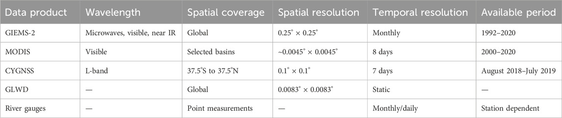
Table 1. Characteristics of the independent products used for comparison analysis.
2.1.1 Extended GIEMS-2 (1992–2020)
GIEMS-2 (1992–2015), as described in Prigent et al. (2020), is essentially based on passive microwave observations from the SSM/I and SSMIS satellites that include measurements from 18 to 90 GHz. First, a neural network is used to derive monthly passive emissivities at 19 and 37 GHz. Then, an unsupervised classification process is used to identify inundated pixels (snow pixels are flagged, i.e., not processed). For this, a combination of active microwave satellite observations (scatterometer) and NDVI helps to better characterize the vegetation and to subtract its contribution from the passive microwave signal. Finally, monthly global maps of surface water extent are calculated from microwave emissivities time series at a spatial resolution of 0.25° × 0.25°, using the active microwave data and NDVI to account for vegetation. The seamless consistent time series relies on carefully inter-calibrated SSM/I and SSMIS observations, provided by the EUMETSAT Climate Satellite Application Facilities (Fennig et al., 2020). The initial GIEMS-2 dataset (1992–2015) (Prigent et al., 2020) has been extended to 2020 for this study, taking into account the latest processing and inter-calibration changes. GIEMS-2 dataset includes all continental water surfaces, including wetlands, rivers, reservoirs, and lakes, with the exception of the largest lakes that have been masked.
2.1.2 MODIS-based surface water extent (2000–2020)
Inundation extent has also been derived from the radiances acquired by the MODIS instrument launched on the Terra satellite in 1999. MOD09A1 version 6, a level 3 product, is used. The data can be freely downloaded from https://search.earthdata.nasa.gov/search. The approach is based on the multi-thresholding of the Enhanced Vegetation Index (EVI) and Land Surface Water Index (LSWI) spectral indices derived from the MODIS radiances, and their difference (Frappart et al., 2018; Normandin et al., 2018; Normandin et al., 2024). It is a simplified version of the method earlier proposed by Sakamoto et al. (2007). The resulting maps have a spatial resolution of 500 m, a temporal resolution of 8 days, and are available over 2000–2022. Pixels are classified as inundated, mixed (containing both water and vegetation) or non-inundated for each map. Due to limitations related to visible observations, such as vegetation and cloud cover, the data are not accessible globally but have been calculated over specific basins. The available basins are the Mackenzie Delta, the lower Ob, the Mississippi, the Yangtze, the Mekong, the Nile, the Inner Niger Delta, the Lake Chad, La Plata, and the Eyre.
2.1.3 CYGNSS-based surface water extent (August 2018–July 2019)
The Cyclone Global Navigation Satellite System (CYGNSS) is a spaceborne GNSS-Reflectometry (GNSS-R) mission composed of 8 micro-satellites launched in 2016 (Ruf et al., 2016). Each satellite carries a receiver that collects the reflected GPS L1 signals (wavelength ∼19 cm) in a bi-static configuration. The 8 satellites collect up to 64 measurements per second (32 before July 2019) between ±40° latitude and so provide a very high repetitivity. The main products of CYGNSS are the L1 Delay Doppler Maps (DDM). Highly coherent signals are typically associated with surface water, so the coherent reflectivity from CYGNSS was used to detect the presence of inundation (Zeiger et al., 2022). These coherent reflectivities were converted to water fraction through a linear model trained on inundation maps from MODIS (Frappart et al., 2018; Normandin et al., 2018) for low vegetation cover and from the L-band SAR instrument on board JERS-1 (Hess et al., 2003; Hess et al., 2015) for dense vegetation cover. The linear model takes into account the attenuation by the vegetation using a third-order polynomial fit against the GlobBiomass Above Ground Biomass (AGB) maps from Santoro et al. (2021). The resulting SWE product has a 0.1° × 0.1° spatial resolution and a 7-day temporal resolution. It was computed for 1 year (August 2018–July 2019) and the spatial coverage ranges from 37.5°S to 37.5°N. The dataset is available at https://doi.org/10.6096/3003 and more details can be found in Zeiger et al. (2023).
2.1.4 GLWD
The Global Lakes and Wetlands Database level 3 (Lehner and Döll, 2004) provides globally a static distribution of the fraction of 12 wetlands and open water classes at 30-s resolution. It is not based directly on satellite observations, but derived from 17 other datasets (see Lehner and Döll (2004) for more details). GLWD is a widely used point of comparison for surface water studies.
2.1.5 River discharges
River discharge measurements were collected from the Global Streamflow and Metadata Archive (GSIM) (Do et al., 2018; Gudmundsson et al., 2018), the HYBAM Observation Service (https://hybam.obs-mip.fr/fr/donnees/), the Water Office Canada (http://wateroffice.ec.gc.ca/), and personal exchange with B. Pham-Duc for data over the Mekong. When several stations were available in a basin, the selection of the station aimed to ensure its location was as integrative as possible with respect to the entire basin. Detailed information about river discharges stations used can be found in Supplementary Table S1.
2.2 Auxiliary datasets
This section describes datasets used for discussion in this work that have an interdependence with GIEMS-2. SWAMPS uses identical microwave observations as GIEMS-2, while TOPMODEL, which is a model-derived product, is calibrated with GIEMS-2.
2.2.1 SWAMPS (1990–2020)
The Surface Water Microwave Product Series (SWAMPS) (Jensen and Mcdonald, 2019) product is derived using similar observations to GIEMS-2. In fact, it is based on a combination of passive and active microwaves with a priori knowledge of land cover. This product provides global SWE at 0.25° × 0.25° for 1992–2020.
2.2.2 TOPMODEL (1980–2020)
Xi et al. (2022) developed a set of monthly global wetland products using TOPMODEL. TOPMODEL simulates grid-level wetland fraction by input of soil moisture and topography index, so that the wetland fraction from TOPMODEL follows the variation in soil moisture. In the version used here, TOPMODEL is run with the ERA5 soil moisture as input, and has been calibrated with a GIEMS-2 mean annual seasonal climatology. The TOPMODEL simulation covers the period 1980–2020 and its spatial resolution is 0.25° × 0.25°. The inter-annual variability of the model is completely independent of GIEMS-2: the model is calibrated once with the GIEMS-2 mean annual seasonal climatology and is then run over the full time period without any additional tuning to the GIEMS-2 long-term series.
3 Methods
3.1 Spatio-temporal data resampling
In order to achieve a consistent comparison between GIEMS-2 and the other data sources, i.e., MODIS, CYGNSS, GLWD, and river discharges, a spatio-temporal resampling of these products is needed to ensure comparable temporal and spatial resolutions.
In the case of MODIS, the sum of inundated and mixed pixels is considered. The data are converted from 500 m to 0.25° by calculating the fraction of inundated and mixed 500 m × 500 m pixels within each larger 0.25° × 0.25° pixel. A monthly average is then calculated from the initial 8-day resolution.
For CYGNSS, monthly means are calculated from the 7-day resolution data. A first-order Conservative Remapping (Jones, 1999) is employed to regrid the data from 0.1° to 0.25°. This remapping numerical method preserves the integral of the original data.
In the case of GLWD, the fraction of each class is calculated over 0.25° × 0.25° pixels. A sum across all classes gives the total 0.25° fraction occupied by wetlands or inundated areas. It is recognized that this may result in an overestimate because some GLWD categories include non-flooded areas, such as those containing peatlands. The GLWD wetland complex categories are expressed in percentage ranges, then the median value is selected as an approximation for these classes (e.g., for the 50%–100% wetland category, pixels are considered to be 75% wetland). Note that GLWD is mostly used here as a comparison in terms of spatial patterns, and the authors verified that choosing the minimum, maximum or median value had little effect on the spatial distribution of GLWDv2.
For river discharges, monthly data are used when available. For the Tan Chau station (Mekong), monthly averages are derived from daily data. To enhance comparability, a normalization process sets the maximum value of either the seasonality or the entire time series for each gauge to 1.
3.2 Snow and ocean masks
The microwave observations used in GIEMS-2 and CYGNSS are affected by the presence of snow. As a result, the surface water fraction cannot be reliably quantified if snow is present in a pixel. Also, MODIS visible/IR observations do not penetrate the snow cover. Then, water bodies beneath the snow are not considered here, only snow-free water surfaces. To handle snow-covered pixels uniformly, a dynamic 0.25° snow mask is developed using ECMWF ERA5 data (Copernicus Climate Change Service, 2019), which identifies pixels with a snow fraction greater than 2%. For each month, snow-covered pixels have their inundation fraction systematically set to 0 in GIEMS-2, MODIS, and CYGNSS datasets.
Passive microwave observations are sensitive to the presence of water, including oceans. Then, a static 0.25° ocean mask is developed by excluding pixels with more than 10% ocean using HydroSHEDS HydroBASINS shapefiles (Lehner and Grill, 2013) and excluding also the Caspian Sea using HydroSHEDS HydroLakes (Messager et al., 2016). This ocean mask is applied to 0.25° GIEMS2, MODIS, CYGNSS, and GLWD products.
3.3 Definition of the evaluation metrics
For each grid point and each selected basin, a 12-month climatology of the SWE (or mean annual seasonal cycle) is calculated for each month over the entire available period. Then, the monthly maximum, minimum, and mean of each pixel is selected, leading to the generation of three static maps of Mean Annual maximum, minimum, and mean (MAmax, MAmin, and MAmean, respectively). GLWD is a static map encompassing all wetlands and inundated areas, including those periodically wet: GLWD is expected to be approximately equivalent to a MAmax when compared to other datasets, acknowledging that GLWD is likely to be closer to a long-term maximum and not a Mean Annual maximum. Note that CYGNSS-based SWE is available for only 1 year, and as a consequence the seasonal cycle of this dataset is only representative of 1 year (along with the related MAmax, MAmin and MAmean).
The agreement between the mean annual seasonal cycle of the different products is evaluated through the calculation of their Pearson cross-correlation coefficients (rsea), providing the maximum correlation between two 12-month time series and the corresponding lag (in month) to obtain the maximum correlation. The Root Mean Square Difference is also calculated between the mean seasonal cycle of GIEMS-2 (12 values) and the mean seasonal cycle of the other products (12 values). It is noted RMSDsea (note that no lag is considered in this calculation). For an easier comparison between basins, the RMSDsea is also normalized by the GIEMS-2 MAmean SWE over that basin.
The evaluation of the inter-annual variations is performed through the calculation of the cross-correlations between the long-term time series of monthly values (rts). The cross-correlation of the anomalies is also calculated (rano), removing the mean annual seasonal cycle from each long-term time series.
4 Comparisons of GIEMS with the selected products
The GIEMS-2 dataset is here compared with the other independent products. First, spatial considerations (total extent and spatial patterns) on global and basin scales are presented. Seasonality, long-term time series and their anomalies at the basin scale are then analyzed.
4.1 Global spatial distribution
Figure 1 represents the SWE MAmax of GIEMS-2, CYGNSS, and MODIS products and the sum of GLWD classes at 0.25°. Large basins such as the Amazon, the Mississippi, or the Ganges can be consistently identified on GIEMS-2, CYGNSS, and GLWD MAmax maps. Some large differences exist, and can be partially explained. First, large lakes have been removed from GIEMS-2 (e.g., Victoria Lake), which is not the case for MODIS. For CYGNSS, they were filtered out during the processing due to the dominant incoherent scattering found over large lakes (Zeiger et al., 2022) and further refilled with a 100% water fraction. Second, the CYGNSS product includes only 1 year of data, resulting in an annual maximum that depends on the conditions of that particular year. Finally, some GLWD classes include peatlands that are not flooded (see peatland rich regions such as North America and the Congo basin) and some areas that are only occasionally flooded.
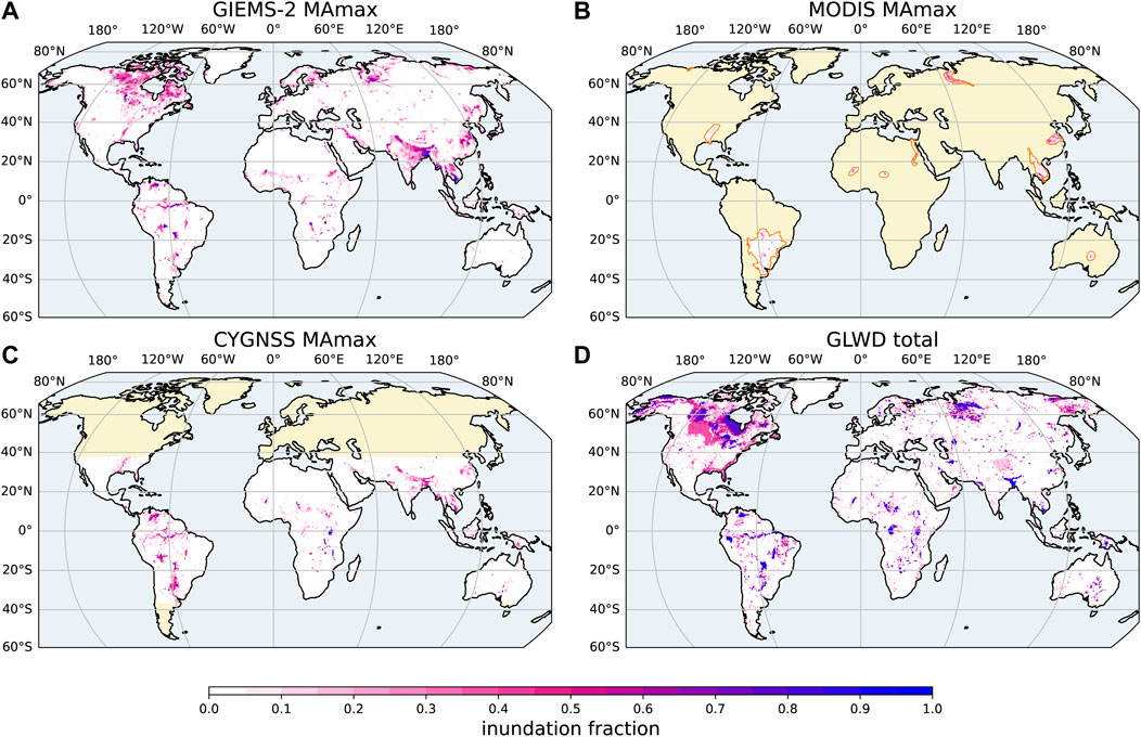
Figure 1. Mean Annual maximum (MAmax) of (A) GIEMS-2, (B) MODIS, (C) CYGNSS. The same basin and dynamic snow masks are applied to GIEMS-2, MODIS, and CYGNSS 0.25° monthly gridded datasets. (D) GLWD total (sum over all classes). Khaki background indicates regions that are not covered by the products.
GLWD presents a total surface area of 10.6 Mkm2: this is much higher than GIEMS-2 MAmax of 6.18 Mkm2, which is not surprising given the points raised just above. If we focus on 37.5°S-37.5°N latitudinal band, GIEMS-2 presents a MAmax values of 3.65 Mkm2 which is higher than the CYGNSS MAmax of 2.46 Mkm2. The same occurs for MAmean with GIEMS-2 MAmean at 1.58 Mkm2 and CYGNSS at 1.25 Mkm2, while MAmin present very close values: 0.57 Mkm2 for GIEMS-2 and 0.59 Mkm2 for CYGNSS.
4.2 Per-basin spatial distribution
Figure 2 presents the SWE MAmax of GIEMS-2, MODIS, CYGNSS, and GLWD total SWE over four basins, each representative of distinct latitudinal bands and environments: the lower Ob, the Mississippi, the Amazon, and La Plata. Additional basins (the Mackenzie delta, the Yangtze, the Ganges, the Mekong, the Orinoco, and the Congo) are shown in Supplementary Figure S1. Despite the same 0.25° regridding used for the maps, GIEMS-2 shows a coarser and more diffuse pattern compared to CYGNSS and MODIS, due to the original low spatial resolution of the passive microwave observations.
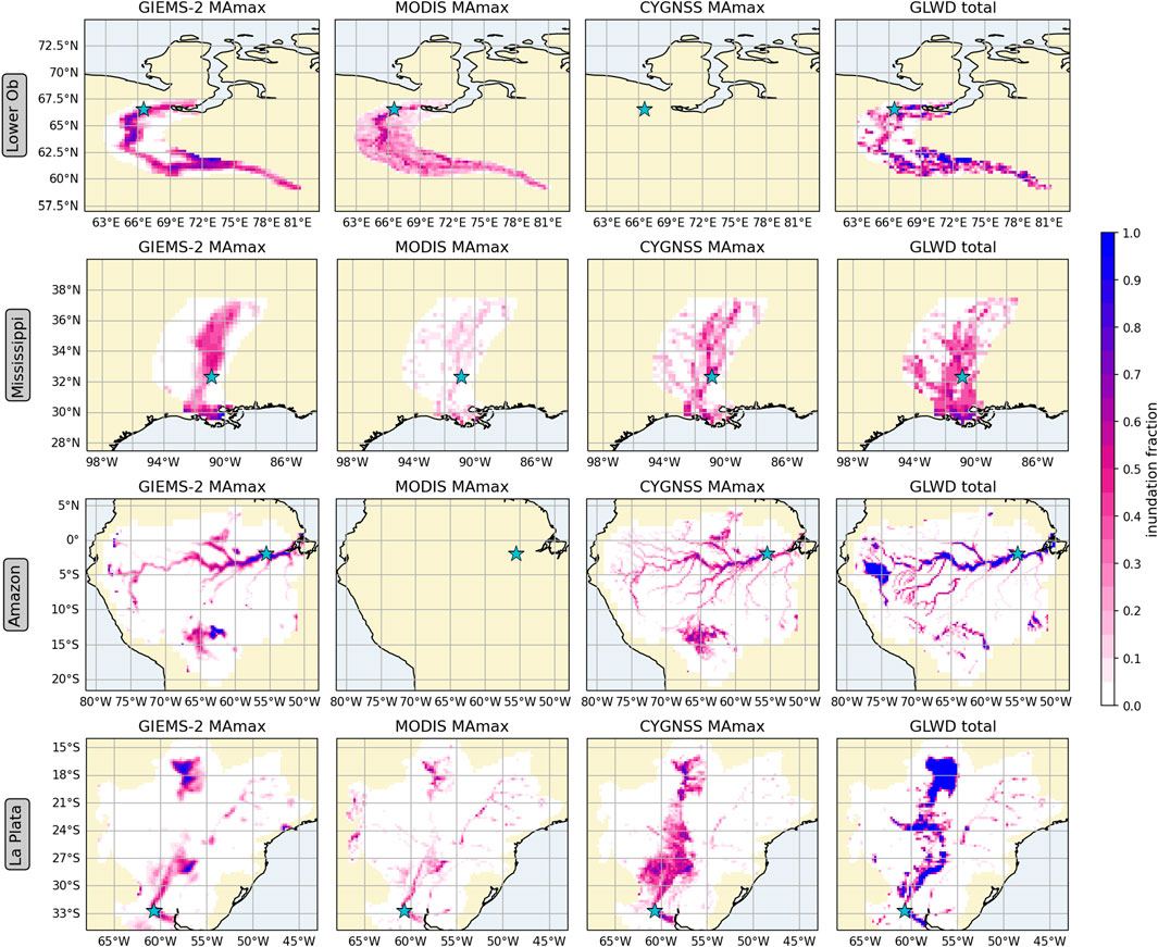
Figure 2. Mean Annual maximum (MAmax) of the different datasets per basin when available. The same basin and snow masks are applied to all 0.25° monthly gridded datasets. Khaki background indicates regions that are not covered by the products. Blue stars represent the selected river gauge location. With 1 year of CYGNSS product, the MAmax corresponds to that year maximum.
The combined visual analysis of Figure 2 and Supplementary Figure S1 reveals consistent spatial patterns between the different products over the basins studied. GIEMS-2 and CYGNSS show very similar patterns, probably influenced by the fact that both datasets are mostly derived from microwave observations, as highlighted by Zeiger et al. (2023). However, it should be noted that the frequency bands observed by GIEMS-2 (18–90 GHz) and CYGNSS (1–2 GHz) are different, and that GIEMS-2 is based on passive microwaves while CYGNSS is based on active microwaves, which are different technologies. The visual consistency is confirmed by the spatial correlation analysis shown in Figure 3. Over the 10 basins studied, the spatial correlations of GIEMS-2 MAmax with MODIS MAmax range from 0.55 to 0.77, while with CYGNSS MAmax, the correlations range from 0.67 to 0.87.
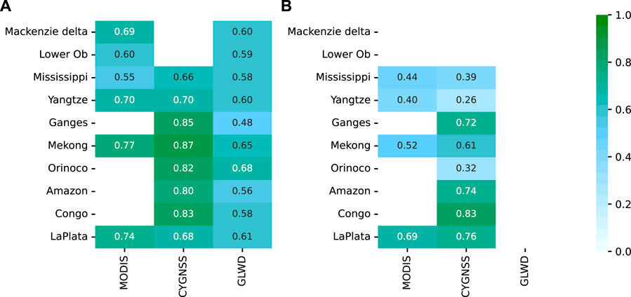
Figure 3. (A) MAmax and (B) MAmin spatial correlation of the different products with GIEMS-2 over selected basins. Cross-correlation is achieved at 0.25° over snow-free pixels.
For the lower Ob basin, MODIS shows more extensive detection of wet areas around the lower Ob riverbed compared to GIEMS-2, but this detection is not confirmed by GLWD. The resulting MAmax over the lower Ob basin is however similar for MODIS (67.7 103 km2) and GIEMS-2 (73.8 103 km2). For the Mississippi, MODIS shows lower MAmax (21.2 103 km2) across the basin compared to the other two datasets (49.0 and 46.3 103 km2 for resp. GIEMS-2 and CYGNSS). This is consistent with the presence of inundated forests along the Mississippi River, which may not be detected by visible and NIR observations. Over the Amazon basin, GIEMS-2 and CYGNSS present very close signatures with a spatial correlation of 0.80, but GIEMS-2 misses small streams as expected, due to its low spatial resolution. GLWD shows roughly the same spatial pattern (r = 0.56), but with finer structures, and elevated values attributed to a swamp in the western part of the basin (5°N, 75°W) that are not present in GIEMS-2 and CYGNSS. In the northern region of the La Plata basin (18°S, 57°W), GLWD presents larger inundation than the other products due to the presence of floodplains, but these areas are not systematically flooded every year, which can partly explain the different patterns and fraction values as compared to GIEMS-2, MODIS, and CYGNSS. In addition, CYGNSS MAmax is based on the maximum of the 2018–2019 monthly mean, as only 1 year of data is available. This factor may contribute to differences with the other products, especially in the La Plata basin, where the SWE in 2019 was particularly high, as shown later in Figure 6. Indeed, we see that the CYGNSS MAmax fractions in La Plata are higher than the MODIS and GIEMS-2 MAmax.
4.3 Seasonal analysis
Figure 4 shows the mean annual seasonal cycle of SWE estimated by GIEMS-2, MODIS, and CYGNSS over the lower Ob, the Mississippi, the Amazon, and La Plata basins. The mean seasonal cycle of the normalized river discharge is also presented (division by the seasonal discharge maximum). Other studied basins are in Supplementary Figure S2. The cross-correlation coefficients and the corresponding lags are depicted in Figure 5A. Figure 5B presents the MAmean of GIEMS-2, MODIS, and CYGNSS datasets, along with the RMSDsea (the color provides the RMSDsea/MAmeanGIEMS−2). As the CYGNSS SWE seasonal cycle represents only 1 year, cross-correlations between products were also calculated by limiting the data to the same year as CYGNSS for all datasets, and it gave similar results (not shown).
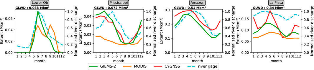
Figure 4. Mean annual seasonal cycle of the different datasets over selected basins, calculated over all available data between 1992 and 2020. The same basin and snow masks are applied to all 0.25° monthly gridded datasets.
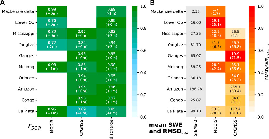
Figure 5. (A) Maximum cross-correlation between the mean annual seasonal cycles of GIEMS-2 SWE and the other data products (MODIS SWE, CYGNSS SWE, and river discharge) over selected catchments, with the corresponding time delays in brackets. Delays from 0 to ±2 months have been tested (applied to GIEMS-2). (B) MAmean and in brackets the RMSDsea, both in 103km2. GIEMS-2 is used as a reference for the RMSDsea calculation. The colors represent the ratio between RMSDsea and MAmeanGIEMS−2.
GIEMS-2 and MODIS exhibit similar seasonal variations (rsea > 0.75), often lagged by 1 month (the Mekong, La Plata). The seasonality on the Yangtze is very different between MODIS and GIEMS-2: GIEMS-2 has a large peak, while MODIS has a less pronounced seasonal cycle. GIEMS-2 and CYGNSS SWE present very similar seasonal temporal variations: the temporal correlation coefficients between the 2 seasonal cycles exceed 0.84 for all basins except La Plata (rsea = 0.69), with no temporal delay in 8 basins out of 10. While the seasonal behaviors between GIEMS-2 and river discharge align in all basins (rsea > 0.85), GIEMS-2 (and CYGNSS) tends to precede river discharge, manifesting as a 1-month lead over the Amazon, the Congo, the Mekong, and La Plata basins, and a 2-month lead for the Mississippi and Yangtze. This temporal offset is consistent with gauge locations close to the river mouth, highlighting the sensitivity of GIEMS-2 and CYGNSS to basin-wide flooding dynamics as observed previously (e.g., Papa et al., 2008; Frappart et al., 2012), which, in turn, influences estuarine behavior where the water concludes its course.
The seasonality in boreal regions is highly dependent on freeze-thaw processes, and indeed we see similar temporal variations over the Mackenzie delta for GIEMS-2 and MODIS. However, over the lower Ob basin, MODIS shows a double flood peak in June and September, while GIEMS-2 and river gauge measurements show only the first peak. The hydrology of the lower Ob basin is complex, and its seasonal variations are attributed to melting ice in spring and rain and evapotranspiration in summer and autumn (Biancamaria et al., 2009; Agafonov et al., 2016). Human influence through damming also alters the hydrological behavior (Yang et al., 2004; Shiklomanov et al., 2021). The literature shows a single seasonal peak (Yang et al., 2004), or a slight second peak (Biancamaria et al., 2009) for river discharge. However, there are only a few studies on water extent for this lower Ob region. Zakharova et al. (2014) obtained SWE by radar altimetry, showing a SWE with a single or double peak, depending on the part of the West Siberian Lowland studied. Mialon et al. (2005) found a double peak seasonality using microwave emissivities. The presence of a second peak in the SWE remains then unclear and would warrant further investigation. The SWOT mission, a Ka-band SAR launched in December 2022, will undoubtedly provide access to new relevant data on this region to improve our understanding of this single or double peak in SWE.
Figure 5B shows that GIEMS-2 exhibits higher mean annual SWE compared to MODIS in all basins, with MODIS peaks being from 30% to 50% lower than GIEMS-2. This is reflected by MODIS RMSDsea/MAmeanGIEMS−2 being above 50% in 5 out of the 6 common basins (see colors in Figure 5B). GIEMS-2 and CYGNSS agree on SWE values on the Mississippi, the Amazon, the Congo, and La Plata basins with RMSDsea/MAmeanGIEMS−2 ≤ 35% over these basins. Over the Orinoco, the amplitudes are also similar (see Supplementary Figure S2), but the RMSDsea/MAmeanGIEMS−2 is higher (0.69). CYGNSS is closer to MODIS SWE values over the Yangtze and the Mekong basins. Over-estimation of the GIEMS products have already been noted in Asia, over saturated soil with low vegetation (e.g., Papa et al., 2015). A correction has been attempted (Prigent et al., 2020), but further adjustments might still be needed.
GLWD consistently exhibits either comparable or higher values than the other SWE products seasonal maximum, except for basins such as the Ganges, the Yangtze, and the Mekong where GIEMS-2 peaks exceed GLWD values. In addition to the possible overestimation of the SWE by GIEMS-2 in these environments, the absence of rice paddies in GLWD also probably lead to underestimation of inundated areas in these regions where rice cultivation is important.
4.4 Analysis of the inter-annual variability
The SWE inter-annual variations are analyzed here. Figure 6 shows the time series and their anomalies for the SWE estimates and for the river discharges above the four selected basins (additional basins available in Supplementary Figure S3). The cross-correlation of the time series rts and the correlation of their anomalies rano between GIEMS-2 and other products can be found in Figures 7A, B, respectively.
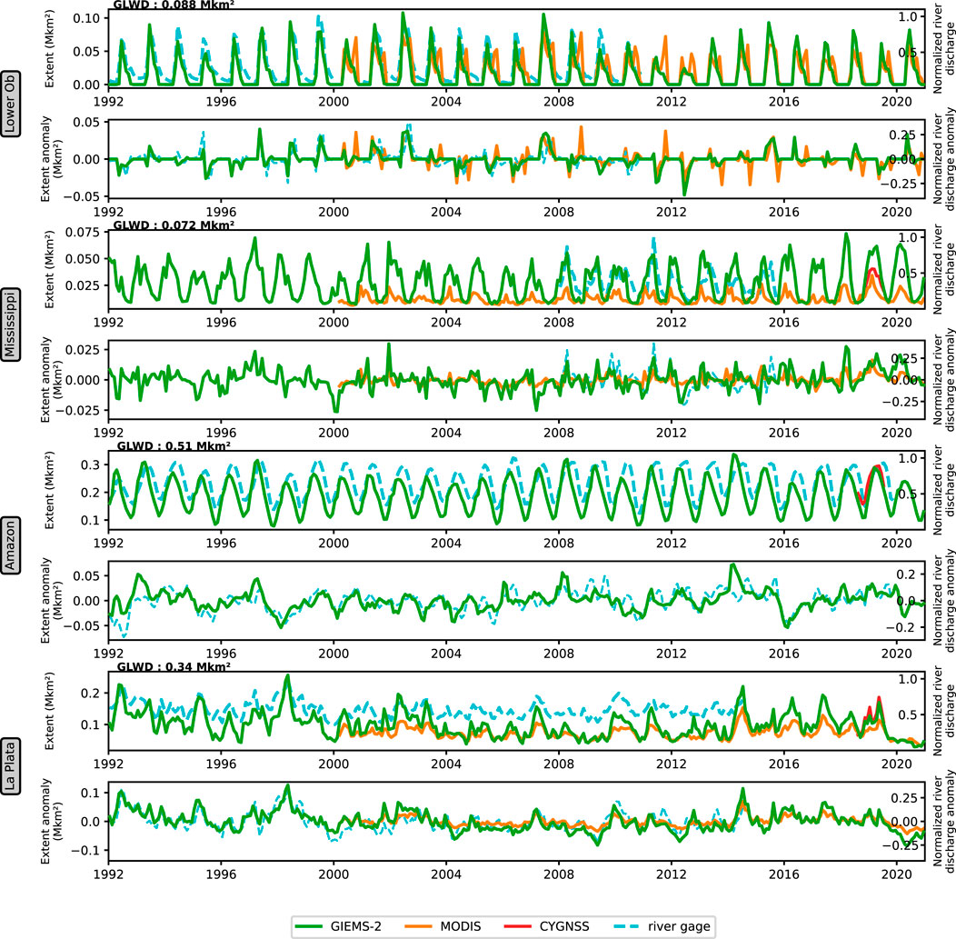
Figure 6. Monthly time series and monthly time series anomalies of the SWE products and river discharges over selected basins. The same basin and snow masks are applied to all 0.25° monthly gridded datasets. With only 1 year of CYGNSS SWE available, no anomalies can be calculated. River discharges are normalized, setting their time series maximum to 1.
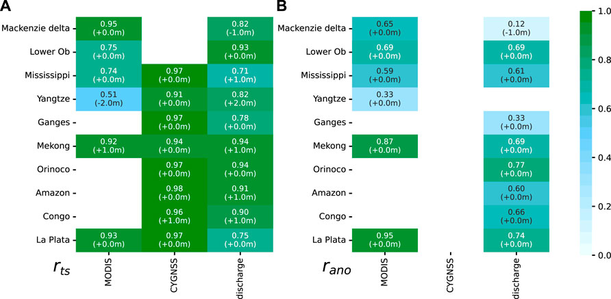
Figure 7. (A) Time series cross-correlations rts and (B) Times series anomalies cross-correlations rano. Cross-correlation with time delay up to ±2 months between GIEMS-2 SWE and the other data products for different basins. The cross-correlations are calculated over the common period of the datasets. As only 1 year of CYGNSS data is available, no anomalies can be calculated.
First, similar patterns can be identified between GIEMS-2 and MODIS in terms of inter-annual variability of SWE and their anomalies. Qualitatively, Figure 6 and Supplementary Figure S3 show good agreement between GIEMS-2 and MODIS over the Mackenzie delta, the lower Ob, the Mekong, La Plata, and the Mississippi, confirmed by cross-correlation coefficients of rts ≥0.74 and rano ≥ 0.59. Lower correlations are recorded over the Yangtze (rts = 0.51 and rano = 0.33). The agreement on the long-term anomalies for 5 out of 6 basins between GIEMS-2 and MODIS is very encouraging. These two datasets are independently derived from two different types of satellite observations, over 20 years. Reaching a good correlation over long-term time series with large seasonal cycles can be expected (with the seasonal cycle driving a large part of the correlation), but once the seasonal cycle is subtracted, only the inter-annual changes are left, and their order of magnitude is much smaller and difficult to capture. The correlations obtained here between GIEMS-2 and MODIS provides confidence in the inter-annual changes observed by both satellite products.
The river discharges at the mouth of the river allow long-term observations of the basin hydrology that should be related to the SWE integrated over the basins. Here again, the long-term time series of GIEMS-2 and discharges as well as their anomalies show good agreements (Figure 6 and Supplementary Figure S3). On the monthly time series, a delay of one or 2 months can be observed between GIEMS-2 and discharges, as already discussed in Section 4.3. The agreement is confirmed by the correlation values, with rts ≥ 0.71 for all basins and rano ≥ 0.60 for 7 of the 9 basins. Note that over the forested tropical basins, the long-term anomalies of GIEMS-2 and river discharge agree well (e.g., rano = 0.60 for the Amazon and rano = 0.66 for the Congo). This notable performance suggests that GIEMS-2 has the ability to detect swamps and floodplains, as well as their inter-annual changes, even under dense tropical forests. Results from the Mackenzie delta and the Ganges (resp., rano = 0.12 and rano = 0.33) could be partly related to the locations of the two river gauges in these basins, rather far from the river mouths and less representative of the full extent of the basins. In fact, the Mackenzie delta gauge is located upstream of the basin, and the Ganges gauge is located in the upper part of the Hasdeo river, which is part of the Ganges basin, but not a tributary of the Ganges. The inter-annual variations at these specific gauges are therefore probably unrepresentative of the entire basins.
GIEMS-2 data spans 30 years and relies on passive microwave observations from several satellites. Using carefully inter-calibrated satellite observations and a robust methodology makes it possible to generate a long time-series of SWE showing an inter-annual variability that agrees with MODIS estimates, as well as with river discharges, under a large range of environments.
5 Discussion
5.1 Limitations and potentials
Comparisons of SWE from multiple sources is challenging. This is corroborated by the wide dispersion found in the literature, with global SWE ranging from 4.5 to 12.9 Mkm2 depending on the products [see Table 1 in Xi et al. (2022)]. All information sources do not consider the same surface types, some including open water bodies such as lakes and rivers, while others remove part of the large open water bodies. Non-inundated peatlands can also be considered in datasets such as GLWD. Irrigated and/or rainfed rice fields are also sometimes included or removed, depending on the datasets. The satellite-derived SWE considered here are extracted from different satellite observations, with different spatial resolutions, as well as with different sensitivities to vegetation.
Variations in the inundation fraction values are observed between the different products. In particular, GIEMS-2 tends to detect more water than MODIS and CYGNSS in areas characterized by high inundation fractions, possibly leading to an overestimation in these areas. Its detection capability seems also to decrease compared to MODIS and CYGNSS in areas with lower flood fractions or fine spatial structures. This is related to the low spatial resolution of the passive microwave observations from which GIEMS-2 is extracted compared to the finer spatial resolution of the MODIS and CYGNSS observations. Prigent et al. (2007) estimated that GIEMS and GIEMS-2 probably underestimates small wetlands comprising less than 10% fractional coverage and overestimates large wetland fractions, due to the low spatial resolution of the initial satellite observations, although the results have been improved from GIEMS to GIEMS-2.
GIEMS-2 is derived from passive microwave observations that can show similar signatures over ocean, desert, and continental surface water (Pham-Duc et al., 2017). That leads to possible over-estimation of the SWE in the coastal regions (ocean contamination in the signal) and in arid regions (misinterpretation of the signal). This risk of confusion is taken into account in the GIEMS-2 processing. However, in an attempt to avoid misclassification, the GIEMS-2 product could be over-cleaned, resulting in lower SWE compared to MODIS in some arid regions (e.g., the north of the Inner Niger Delta in Supplementary Figure S4). Nevertheless, significant differences between the three remotely sensed SWE considered here have been observed over arid regions, e.g., over the Nile basin in Supplementary Figure S4, where the spatial correlation between the three products are low (r
Finally, the strengths of GIEMS-2 lie in its long time series, global nature and consistency in terms of temporal variability, as shown in the results section. This comparison helps to understand the strengths and limitations of the information sources, with notable differences found among the various SWE estimates. Efforts are already underway to take advantage of the complementarity of the different techniques. For example, the high spatial resolution of visible imagery (such as MODIS) will be used to provide accurate estimates of open water, while microwave observations, which are less affected by vegetation, will provide key information in forested areas such as the Amazon floodplains.
5.2 Analysis of differences between GIEMS-2 and SWAMPS
To further highlight specific aspects of a microwave-based SWE product, we briefly discuss here a comparison of GIEMS-2 and SWAMPS. As mentioned in Section 2, SWAMPS and GIEMS-2 are using the same satellite information, passive microwave observations from SSM/I and SSMIS. The differences between SWAMPS and GIEMS are only due to different processing/algorithms to estimate the surface water. SWAMPS shows globally higher SWE MAmax (8.4 Mkm2) than GIEMS-2 (6.2 Mkm2). We found that major differences in total extent occur in 1. coastal areas, 2. snow-covered pixels and 3. desert areas. To compare areas not contaminated by these environments, a test was performed by setting pixels
SWAMPS monthly seasonal cycles are shown over the lower Ob, the Mississippi, the Amazon, and La Plata basins in Figure 8 along with GIEMS-2, MODIS, and CYGNSS estimates (other basins in Supplementary Figure S2). Cross-correlations with GIEMS-2 in terms of mean seasonality, long-term time series, and anomalies are presented in Figure 8. Cross-correlations of anomalies are greater than 0.7 over 6 out of the 10 basins, but differ on the Mackenzie delta, the lower Ob, the Amazon, and the Congo basins. This reflects important differences between GIEMS-2 and SWAMPS products, although the same satellite observations are used. Also, we notice on Figure 8 that SWAMPS presents flat seasonal cycles over the Amazon (SWE seasonal amplitude ∼0.02 Mkm2) and the Congo (SWE seasonal amplitude ∼0.002 Mkm2), two basins with dense vegetation, while GIEMS-2 and CYGNSS show significant seasonal variations over the two basins (SWE seasonal amplitude
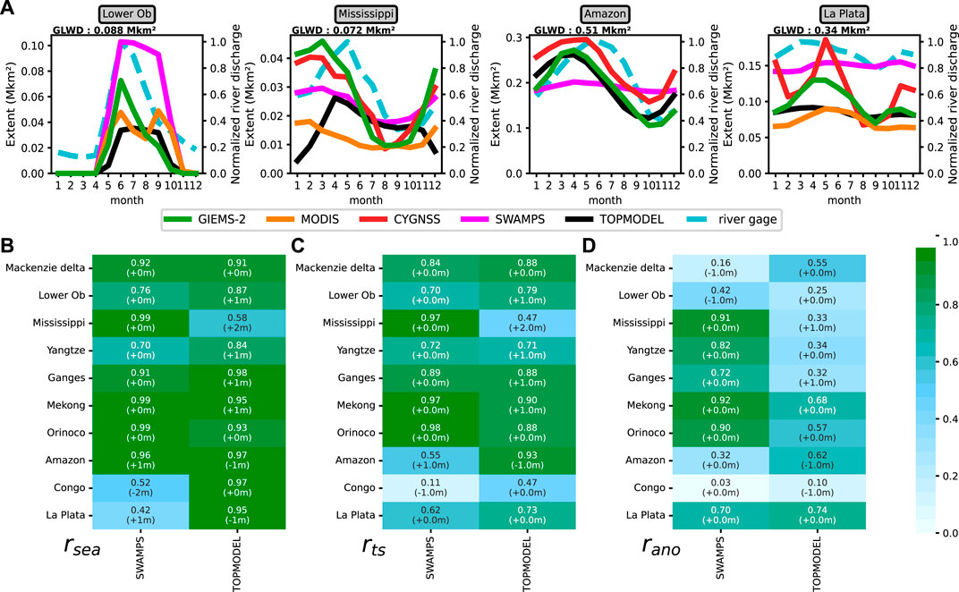
Figure 8. (A) Mean annual seasonal cycle of different datasets over selected basins, calculated over all available data between 1992 and 2020. Cross-correlations between GIEMS-2 and SWAMPS or TOPMODEL over the selected basins for (B) the mean annual seasonal cycle, (C) the long-term time series and (D) the long-term anomalies.
5.3 GIEMS-2 and hydrological models
Hydrological models represent changes in the different components of the water cycle and the fluxes between them. They help to quantify current water resources and are a unique resource for climate projections under different scenarios. In this section, we analyze the SWE outputs derived from the TOPMODEL to illustrate the potential of GIEMS-2 for hydrological modeling.
The spatial correlation coefficient between GIEMS-2 and TOPMODEL SWE MAmax is 0.85 on a global scale. However, their MAmin show different patterns (correlation 0.38), reflecting their independence in temporal variations. The seasonal variations of the TOPMODEL product over the selected basins are shown in Figure 8 and Supplementary Figure S2. The seasonal cross-correlation rsea between GIEMS-2 and TOPMODEL is greater than 0.75 in 9 out of 10 basins (Figure 8), but 7 out of 10 basins show a lag. Compared to the three remote sensing datasets, TOPMODEL has a distinct seasonal cycle over the Mississippi and the Yangtze basins. GIEMS-2 and TOPMODEL agree particularly well on the long-term anomalies over the Mekong, La Plata, and Amazon basins (rano = 0.69, 0.74 and 0.62, respectively), with anomalies over the remaining basins showing less agreement.
Generally, TOPMODEL assumes soil moisture distribution in a grid following the distribution of topography index, which can capture regular wetlands defined as saturated soil. However, floodplains, as the flooded area near the river when the river is full, cannot be simulated well by TOPMODEL because floodplains have different drivers of formation (Nanson and Croke, 1992; Dunne and Aalto, 2013). GIEMS-2 captures seasonal and inter-annual variations of floodplains, explaining different seasonal cycles between GIEMS-2 and TOPMODEL in some basins (e.g., Mississippi), where GIEMS-2 has better correlations with river gauges. These floodplain variations cannot be modeled by TOPMODEL alone. Combining TOPMODEL and a floodplain model has been suggested (Decharme et al., 2012; Lauerwald et al., 2017) to obtain more accurate wetland fractions in basins with significant floodplain fractions. The robust seasonal variations observed in GIEMS-2 and largely validated here will be useful in calibrating or evaluating the coupled model, like any other hydrological model.
6 Conclusion and outlook
GIEMS-2 provides an estimate of the monthly surface water extent from 1992 to 2020 with a spatial resolution of 0.25° × 0.25°. GIEMS-2 is derived primarily from passive microwave observations provided by the SSM/I and SSMIS sensors. It is evaluated here against other independent products.
On the basin scale, the SWE from GIEMS-2, MODIS, and CYGNSS products show consistent spatial patterns. However, differences can be observed in the extent, for both mean annual maximum and minimum. This is explained by the combination of several factors, including the differences in the spatial resolutions of the satellite observations. The mean annual seasonal cycle shows significant agreement (with cross-correlations above 0.8 for most selected basins) between GIEMS-2 and the other satellite-derived products, as well as with the river discharges. Over their common 20 years, the inter-annual variations of GIEMS-2 and MODIS present very similar features, with their anomalies having correlations above 0.6 over basins in diverse environments. Compared to river discharge, GIEMS-2 also shows realistic inter-annual variability, with correlations over 0.6 between long-term anomalies over most basins, including under tropical basins (Amazon and Congo) where passive microwaves are often suspected to be insensitive to surface water variations. Based on carefully inter-calibrated satellite observations and a robust methodology, GIEMS-2 shows no artefacts related to satellite changes over the 30 years, and provides a seamless SWE time record that can be used for climate analysis.
Calibration of a hydrological model (TOPMODEL) with GIEMS-2 shows encouraging results, and improvements are expected by coupling TOPMODEL with a flood model. Modeling approaches are the only means to provide climate predictions for surface waters, with efforts based on robust observational estimates showing promise.
Given that wetlands are responsible for approximately a third of global methane emissions, the global methane budget is significantly influenced by the seasonal and inter-annual dynamics of wetland extents. We showed here that GIEMS-2 provides a 30-year time series of global surface water extent, with very realistic inter-annual variations, and thus can provide key information to the methane emission modelers for the analysis of the inter-annual variation of atmospheric methane. Methane emissions are not uniform across all surface waters and depend on surface characteristics. The next step will consist in combining GIEMS-2 with land cover data and other water body distributions to build a coherent product representing different surface water categories. This effort is intended to facilitate the coherent simulation of methane emissions across various ecosystems.
Data availability statement
The raw data supporting the conclusion of this article will be made available by the authors, without undue reservation.
Author contributions
JB: Conceptualization, Formal Analysis, Investigation, Writing–original draft, Writing–review and editing. CP: Conceptualization, Investigation, Resources, Supervision, Writing–review and editing. CJ: Resources, Writing–review and editing. FF: Resources, Writing–review and editing. CN: Resources, Validation, Writing–review and editing. PZ: Resources, Writing–review and editing. YX: Resources, Writing–review and editing. SP: Investigation, Writing–review and editing.
Funding
The authors declare that financial support was received for the research, authorship, and/or publication of this article. JB is funded by a PhD grant from the Institut National des Sciences de l’Univers (INSU) of the Centre National de la Recherche Scientifique (CNRS). Partial funding has been provided by the ESA CCI RECAPP2 project (4000123002/18/I-NB).
Acknowledgments
The authors would like to thank Binh Pham Duc for generously providing discharge data for the Mekong River. Special thanks go to Marielle Saunois and Elodie Salmon for their dedicated supervision of JB’s PhD, and to Philippe Ciais for the financial support of this research initiative.
Conflict of interest
The authors declare that the research was conducted in the absence of any commercial or financial relationships that could be construed as a potential conflict of interest.
Author FF declared that he was an editorial board member of Frontiers, at the time of submission. This had no impact on the peer review process and the final decision.
Publisher’s note
All claims expressed in this article are solely those of the authors and do not necessarily represent those of their affiliated organizations, or those of the publisher, the editors and the reviewers. Any product that may be evaluated in this article, or claim that may be made by its manufacturer, is not guaranteed or endorsed by the publisher.
Supplementary material
The Supplementary Material for this article can be found online at: https://www.frontiersin.org/articles/10.3389/frsen.2024.1399234/full#supplementary-material
References
Agafonov, L. I., Meko, D. M., and Panyushkina, I. P. (2016). Reconstruction of Ob River, Russia, discharge from ring widths of floodplain trees. J. Hydrology 543, 198–207. doi:10.1016/j.jhydrol.2016.09.031
Biancamaria, S., Bates, P. D., Boone, A., and Mognard, N. M. (2009). Large-scale coupled hydrologic and hydraulic modelling of the Ob river in Siberia. J. Hydrology 379, 136–150. doi:10.1016/j.jhydrol.2009.09.054
Bousquet, P., Ciais, P., Miller, J. B., Dlugokencky, E. J., Hauglustaine, D. A., Prigent, C., et al. (2006). Contribution of anthropogenic and natural sources to atmospheric methane variability. Nature 443, 439–443. doi:10.1038/nature05132
Copernicus Climate Change Service (2019) Era5 monthly averaged data on single levels from 1979 to present. doi:10.24381/CDS.F17050D7
Cretaux, J.-F., Calmant, S., Papa, F., Frappart, F., Paris, A., and Berge-Nguyen, M. (2023). Inland surface waters quantity monitored from remote sensing. Surv. Geophys. 44, 1519–1552. doi:10.1007/s10712-023-09803-x
Decharme, B., Alkama, R., Papa, F., Faroux, S., Douville, H., and Prigent, C. (2012). Global off-line evaluation of the ISBA-TRIP flood model. Clim. Dyn. 38, 1389–1412. doi:10.1007/s00382-011-1054-9
Do, H. X., Gudmundsson, L., Leonard, M., and Westra, S. (2018) The global Streamflow indices and Metadata archive - Part 1: station catalog and catchment boundary. doi:10.1594/PANGAEA.887477
Dunne, T., and Aalto, R. (2013). “9.32 large river floodplains,” in Treatise on geomorphology (Elsevier), 645–678. doi:10.1016/B978-0-12-374739-6.00258-X
Fassoni-Andrade, A. C., Fleischmann, A. S., Papa, F., Paiva, R. C. D. D., Wongchuig, S., Melack, J. M., et al. (2021). Amazon hydrology from Space: scientific advances and future challenges. Rev. Geophys. 59, e2020RG000728. doi:10.1029/2020RG000728
Fennig, K., Schröder, M., Andersson, A., and Hollmann, R. (2020). A fundamental climate data record of SMMR, SSM/I, and SSMIS brightness temperatures. Earth Syst. Sci. Data 12, 647–681. doi:10.5194/essd-12-647-2020
Fernández-Prieto, D., Van Oevelen, P., Su, Z., and Wagner, W. (2012). Editorial “Advances in Earth observation for water cycle science”. Hydrology Earth Syst. Sci. 16, 543–549. doi:10.5194/hess-16-543-2012
Frappart, F., Biancamaria, S., Normandin, C., Blarel, F., Bourrel, L., Aumont, M., et al. (2018). Influence of recent climatic events on the surface water storage of the Tonle Sap Lake. Sci. Total Environ. 636, 1520–1533. doi:10.1016/j.scitotenv.2018.04.326
Frappart, F., Papa, F., Santos Da Silva, J., Ramillien, G., Prigent, C., Seyler, F., et al. (2012). Surface freshwater storage and dynamics in the Amazon basin during the 2005 exceptional drought. Environ. Res. Lett. 7, 044010. doi:10.1088/1748-9326/7/4/044010
Gudmundsson, L., Do, H. X., Leonard, M., and Westra, S. (2018). The global Streamflow indices and Metadata archive (GSIM) - Part 2: time series indices and homogeneity assessment. PANGAEA. doi:10.1594/PANGAEA.887470
Hess, L. L., Melack, J., Novo, E. M., Barbosa, C. C., and Gastil, M. (2003). Dual-season mapping of wetland inundation and vegetation for the central Amazon basin. Remote Sens. Environ. 87, 404–428. doi:10.1016/j.rse.2003.04.001
Hess, L. L., Melack, J. M., Affonso, A. G., Barbosa, C., Gastil-Buhl, M., and Novo, E. M. L. M. (2015). Wetlands of the Lowland Amazon basin: extent, vegetative cover, and dual-season inundated area as mapped with JERS-1 synthetic aperture radar. Wetlands 35, 745–756. doi:10.1007/s13157-015-0666-y
Huang, C., Chen, Y., Zhang, S., and Wu, J. (2018). Detecting, extracting, and monitoring surface water from Space using optical sensors: a review. Rev. Geophys. 56, 333–360. doi:10.1029/2018RG000598
Jensen, K., and Mcdonald, K. (2019). Surface water microwave product series version 3: a near-real time and 25-year historical global inundated area fraction time series from active and passive microwave remote sensing. IEEE Geoscience Remote Sens. Lett. 16, 1402–1406. doi:10.1109/LGRS.2019.2898779
Jones, P. W. (1999). First- and second-order conservative remapping schemes for grids in spherical coordinates. Mon. Weather Rev. 127, 2204–2210. doi:10.1175/1520-0493(1999)127<2204:fasocr>2.0.co;2
Kraft, B., Jung, M., Körner, M., Koirala, S., and Reichstein, M. (2022). Towards hybrid modeling of the global hydrological cycle. Hydrology Earth Syst. Sci. 26, 1579–1614. doi:10.5194/hess-26-1579-2022
Kreibich, H., Van Loon, A. F., Schröter, K., Ward, P. J., Mazzoleni, M., Sairam, N., et al. (2022). The challenge of unprecedented floods and droughts in risk management. Nature 608, 80–86. doi:10.1038/s41586-022-04917-5
Lauerwald, R., Regnier, P., Camino-Serrano, M., Guenet, B., Guimberteau, M., Ducharne, A., et al. (2017). ORCHILEAK (revision 3875): a new model branch to simulate carbon transfers along the terrestrial–aquatic continuum of the Amazon basin. Geosci. Model Dev. 10, 3821–3859. doi:10.5194/gmd-10-3821-2017
Lehner, B., and Döll, P. (2004). Development and validation of a global database of lakes, reservoirs and wetlands. J. Hydrology 296, 1–22. doi:10.1016/j.jhydrol.2004.03.028
Lehner, B., and Grill, G. (2013). Global river hydrography and network routing: baseline data and new approaches to study the world’s large river systems. Hydrol. Process. 27, 2171–2186. doi:10.1002/hyp.9740
Meli, P., Rey Benayas, J. M., Balvanera, P., and Martínez Ramos, M. (2014). Restoration enhances wetland biodiversity and ecosystem Service supply, but results are context-dependent: a meta-analysis. PLoS ONE 9, e93507. doi:10.1371/journal.pone.0093507
Messager, M. L., Lehner, B., Grill, G., Nedeva, I., and Schmitt, O. (2016). Estimating the volume and age of water stored in global lakes using a geo-statistical approach. Nat. Commun. 7, 13603. doi:10.1038/ncomms13603
Mialon, A., Royer, A., and Fily, M. (2005). Wetland seasonal dynamics and interannual variability over northern high latitudes, derived from microwave satellite data. J. Geophys. Res. Atmos. 110, 2004JD005697. doi:10.1029/2004JD005697
Nanson, G., and Croke, J. (1992). A genetic classification of floodplains. Geomorphology 4, 459–486. doi:10.1016/0169-555X(92)90039-Q
Normandin, C., Frappart, F., Bourrel, L., Diepkilé, A. T., Mougin, E., Zwarts, L., et al. (2024). Quantification of surface water extent and volume in the Inner Niger Delta (IND) over 2000–2022 using multispectral imagery and radar altimetry. Geocarto Int. 39, 2311203. doi:10.1080/10106049.2024.2311203
Normandin, C., Frappart, F., Lubac, B., Bélanger, S., Marieu, V., Blarel, F., et al. (2018). Quantification of surface water volume changes in the Mackenzie Delta using satellite multi-mission data. Hydrology Earth Syst. Sci. 22, 1543–1561. doi:10.5194/hess-22-1543-2018
Papa, F., and Frappart, F. (2021). Surface water storage in rivers and wetlands derived from satellite observations: a review of current advances and future opportunities for hydrological Sciences. Remote Sens. 13, 4162. doi:10.3390/rs13204162
Papa, F., Frappart, F., Malbeteau, Y., Shamsudduha, M., Vuruputur, V., Sekhar, M., et al. (2015). Satellite-derived surface and sub-surface water storage in the ganges–brahmaputra river basin. J. Hydrology Regional Stud. 4, 15–35. doi:10.1016/j.ejrh.2015.03.004
Papa, F., Güntner, A., Frappart, F., Prigent, C., and Rossow, W. B. (2008). Variations of surface water extent and water storage in large river basins: a comparison of different global data sources. Geophys. Res. Lett. 35, 2008GL033857. doi:10.1029/2008GL033857
Papa, F., Prigent, C., Aires, F., Jimenez, C., Rossow, W. B., and Matthews, E. (2010). Interannual variability of surface water extent at the global scale, 1993–2004. J. Geophys. Res. Atmos. 115, 2009JD012674. doi:10.1029/2009JD012674
Pekel, J.-F., Cottam, A., Gorelick, N., and Belward, A. S. (2016). High-resolution mapping of global surface water and its long-term changes. Nature 540, 418–422. doi:10.1038/nature20584
Peng, S., Lin, X., Thompson, R. L., Xi, Y., Liu, G., Hauglustaine, D., et al. (2022). Wetland emission and atmospheric sink changes explain methane growth in 2020. Nature 612, 477–482. doi:10.1038/s41586-022-05447-w
Pham-Duc, B., Prigent, C., Aires, F., and Papa, F. (2017). Comparisons of global terrestrial surface water datasets over 15 years. J. Hydrometeorol. 18, 993–1007. doi:10.1175/JHM-D-16-0206.1
Poulter, B., Fluet-Chouinard, E., Hugelius, G., Koven, C., Fatoyinbo, L., Page, S. E., et al. (2021). “A review of global wetland carbon stocks and management challenges,” in Geophysical monograph series. Editors K. W. Krauss, Z. Zhu, and C. L. Stagg First edn. (Wiley), 1–20. doi:10.1002/9781119639305.ch1
Prigent, C., Jimenez, C., and Bousquet, P. (2020). Satellite-derived global surface water extent and dynamics over the last 25 Years (GIEMS-2). J. Geophys. Res. Atmos. 125. doi:10.1029/2019JD030711
Prigent, C., Matthews, E., Aires, F., and Rossow, W. B. (2001). Remote sensing of global wetland dynamics with multiple satellite data sets. Geophys. Res. Lett. 28, 4631–4634. doi:10.1029/2001GL013263
Prigent, C., Papa, F., Aires, F., Rossow, W. B., and Matthews, E. (2007). Global inundation dynamics inferred from multiple satellite observations, 1993–2000. J. Geophys. Res. 112, D12107. doi:10.1029/2006JD007847
Ruf, C. S., Atlas, R., Chang, P. S., Clarizia, M. P., Garrison, J. L., Gleason, S., et al. (2016). New Ocean winds satellite mission to probe hurricanes and tropical convection. Bull. Am. Meteorological Soc. 97, 385–395. doi:10.1175/BAMS-D-14-00218.1
Sakamoto, T., Van Nguyen, N., Kotera, A., Ohno, H., Ishitsuka, N., and Yokozawa, M. (2007). Detecting temporal changes in the extent of annual flooding within the Cambodia and the Vietnamese Mekong Delta from MODIS time-series imagery. Remote Sens. Environ. 109, 295–313. doi:10.1016/j.rse.2007.01.011
Santoro, M., Cartus, O., Carvalhais, N., Rozendaal, D. M. A., Avitabile, V., Araza, A., et al. (2021). The global forest above-ground biomass pool for 2010 estimated from high-resolution satellite observations. Earth Syst. Sci. Data 13, 3927–3950. doi:10.5194/essd-13-3927-2021
Saunois, M., Stavert, A. R., Poulter, B., Bousquet, P., Canadell, J. G., Jackson, R. B., et al. (2020). The global methane budget 2000–2017. Earth Syst. Sci. Data 12, 1561–1623. doi:10.5194/essd-12-1561-2020
Shen, X., Wang, D., Mao, K., Anagnostou, E., and Hong, Y. (2019). Inundation extent mapping by synthetic aperture radar: a review. Remote Sens. 11, 879. doi:10.3390/rs11070879
Shiklomanov, A., Déry, S., Tretiakov, M., Yang, D., Magritsky, D., Georgiadi, A., et al. (2021). “River freshwater flux to the arctic ocean,” in Arctic hydrology, permafrost and ecosystems. Editors D. Yang, and D. L. Kane (Cham: Springer International Publishing), 703–738. doi:10.1007/978-3-030-50930-9_24
Torres-Alvarado, R., Ramírez-Vives, F., and Fernández, F. J. (2005). Methanogenesis and methane oxidation in wetlands. Implications in the global carbon cycle Metanogénesis y metano-oxidación en humedales. Implicaciones en el ciclo del carbono global. Hidrobiológica 15.
Wania, R., Melton, J. R., Hodson, E. L., Poulter, B., Ringeval, B., Spahni, R., et al. (2013). Present state of global wetland extent and wetland methane modelling: methodology of a model inter-comparison project (WETCHIMP). Geosci. Model Dev. 6, 617–641. doi:10.5194/gmd-6-617-2013
Xi, Y., Peng, S., Ducharne, A., Ciais, P., Gumbricht, T., Jimenez, C., et al. (2022). Gridded maps of wetlands dynamics over mid-low latitudes for 1980–2020 based on TOPMODEL. Sci. Data 9, 347. doi:10.1038/s41597-022-01460-w
Yang, D., Ye, B., and Shiklomanov, A. (2004). Discharge characteristics and changes over the Ob river watershed in siberia. J. Hydrometeorol. 5, 595–610. doi:10.1175/1525-7541(2004)005<0595:dcacot>2.0.co;2
Zakharova, E. A., Kouraev, A. V., Rémy, F., Zemtsov, V. A., and Kirpotin, S. N. (2014). Seasonal variability of the Western Siberia wetlands from satellite radar altimetry. J. Hydrology 512, 366–378. doi:10.1016/j.jhydrol.2014.03.002
Zeiger, P., Frappart, F., Darrozes, J., Prigent, C., and Jiménez, C. (2022). Analysis of CYGNSS coherent reflectivity over land for the characterization of pan-tropical inundation dynamics. Remote Sens. Environ. 282, 113278. doi:10.1016/j.rse.2022.113278
Keywords: remote sensing, surface water extent, wetlands, global hydrology, hydrology modeling, methane modeling
Citation: Bernard J, Prigent C, Jimenez C, Frappart F, Normandin C, Zeiger P, Xi Y and Peng S (2024) Assessing the time variability of GIEMS-2 satellite-derived surface water extent over 30 years. Front. Remote Sens. 5:1399234. doi: 10.3389/frsen.2024.1399234
Received: 11 March 2024; Accepted: 17 April 2024;
Published: 14 May 2024.
Edited by:
Xiaojun Li, INRAE Nouvelle-Aquitaine Bordeaux, FranceReviewed by:
Jian Zhang, Université de Bordeaux, FranceYi Zheng, Sun Yat-sen University, China
Mengjia Wang, Zhengzhou University, China
Copyright © 2024 Bernard, Prigent, Jimenez, Frappart, Normandin, Zeiger, Xi and Peng. This is an open-access article distributed under the terms of the Creative Commons Attribution License (CC BY). The use, distribution or reproduction in other forums is permitted, provided the original author(s) and the copyright owner(s) are credited and that the original publication in this journal is cited, in accordance with accepted academic practice. No use, distribution or reproduction is permitted which does not comply with these terms.
*Correspondence: Juliette Bernard, anVsaWV0dGUuYmVybmFyZEBvYnNwbS5mcg==