
95% of researchers rate our articles as excellent or good
Learn more about the work of our research integrity team to safeguard the quality of each article we publish.
Find out more
ORIGINAL RESEARCH article
Front. Remote Sens. , 16 July 2024
Sec. Data Fusion and Assimilation
Volume 5 - 2024 | https://doi.org/10.3389/frsen.2024.1395442
 Leong Wai Siu1*
 Xubin Zeng1
 Armin Sorooshian1,2
 Brian Cairns3
 Richard A. Ferrare4
 Johnathan W. Hair4
 Chris A. Hostetler4
 David Painemal4,5
 Joseph S. Schlosser4,6
With the ongoing expansion of global observation networks, it is expected that we shall routinely analyze records of geophysical variables such as temperature from multiple collocated instruments. Validating datasets in this situation is not a trivial task because every observing system has its own bias and noise. Triple collocation is a general statistical framework to estimate the error characteristics in three or more observational-based datasets. In a triple colocation analysis, several metrics are routinely reported but traditional multiple-panel plots are not the most effective way to display information. A new formula of error variance is derived for connecting the key terms in the triple collocation theory. A diagram based on this formula is devised to facilitate triple collocation analysis of any data from observations, as illustrated using three aerosol optical depth datasets from the recent Aerosol Cloud meTeorology Interactions oVer the western ATlantic Experiment (ACTIVATE). An observational-based skill score is also derived to evaluate the quality of three datasets by taking into account both error variance and correlation coefficient. Several applications are discussed and sample plotting routines are provided.
The development of atmospheric sciences and other branches of Earth system science is inextricably linked to our capability of improving and expanding current atmospheric observing systems (Crutzen and Ramanathan, 2000; Stith et al., 2018; Bluestein et al., 2022). For instance, a dense weather station network provides us with synoptic weather conditions while sounding profiles from radiosondes and dropsondes give us a wealth of information for the vertical structure of the atmosphere over land and ocean (Stith et al., 2018). In addition to in situ observations, remotely sensed instruments such as weather radars are able to detect severe weather systems in a timely manner. The advent of satellite meteorology has reshaped our data inventory by making global observations possible (Atlas, 1997). Research aircraft in field campaigns provides a unique platform to collect measurements from both in situ and remotely sensed instruments for specific research problems with pressing societal needs (Bluestein et al., 2022).
With more and more new observing systems available, it has become commonplace for more than one instrument observing the same geophysical variable at the same location. Data validation and calibration then become necessary because no observing systems are perfectly built. Stoffelen (1998) recognized this issue and proposed a general statistical framework called triple collocation. For any geophysical variables, triple collocation estimates the error characteristics of three independent datasets without requiring any dataset being the ground truth. Since then, the method has been applied to a wide range of variables such as soil moisture (e.g., Dorigo et al., 2010), sea surface temperature (e.g., O’Carroll et al., 2008), and leaf area index (e.g., Fang et al., 2012), to name a few. The theory of triple collocation has also been clarified, tested, and extended over the years (e.g., Zwieback et al., 2012; Draper et al., 2013; McColl et al., 2014; Su et al., 2014; Yilmaz and Crow, 2014; Gruber et al., 2016; Tsamalis, 2022).
Several performance metrics such as standard error (Stoffelen, 1998) and correlation coefficient (McColl et al., 2014) have been developed for triple collocation analysis. These metrics are usually reported in the form of a map that shows one aspect such as a metric for one dataset (e.g., Dorigo et al., 2010) or a figure that shows another aspect for three datasets (e.g., Tsamalis, 2022). Multiple-panel plots are common in the literature (e.g., McColl et al., 2014; Deng et al., 2023) and some examples are given in Supplementary Material. But this kind of plot is not the most effective way to summarize results. A table that shows multiple aspects may help but different researchers have varying designs and notations (e.g., Su et al., 2014). The purpose of this study is to present a single diagram for the triple collocation analysis that can succinctly compare multiple aspects of multiple datasets. The diagram is facilitated by deriving a new formula of error variance. Some applications of the new triple collocation diagram are illustrated using datasets collected from a recent field campaign, i.e., the Aerosol Cloud meTeorology Interactions oVer the western ATlantic Experiment (ACTIVATE).
We first briefly review the derivation of classical and extended triple collocation. An error model is needed to specify each dataset as a function of the unknown ground truth (Zwieback et al., 2012). So far in the literature, linear error models are the most popular type with one example being the affine model,
where
Based on the affine error model, the variance/covariance equations for the collocated datasets are then given as.
where
Three further assumptions are usually made to simplify the equations (Gruber et al., 2020). First, the mean random error is zero
The six equations from Eqs. 4, 5 now have seven unknowns (
In practice, the signal variance
To extend the classical triple collocation analysis, McColl et al. (2014) derived a new metric, the correlation coefficient, from the ordinary least squares framework.
where
To construct the triple collocation diagram, an alternative error variance equation is needed to connect all variance terms in Eq. 6 with the correlation coefficient (Eqs 10–12). To start with, we use the following basic statistical identities (Dekking et al., 2005; Thomson and Emery, 2014).
where
Combining two identities (Eqs 13, 14) gives
where
Applying the above identity (Eq. 15) to the error model Eq. 1 gives Eq. 16, and subsequently Eqs 17, 18.
where the left hand side (lhs) of Eq. 17 uses Eq. 1, the lhs of Eq. 18 uses Eq. 13. On the right hand side (rhs) of Eq. 18, the correlation coefficient
The alternative error variance Eq. 18 is inspired by the Taylor diagram (Taylor, 2001) which is based on the law of cosines. The alternative equation also resembles the law of cosines (Figure 1A): three sides for three standard deviation terms (error standard deviation
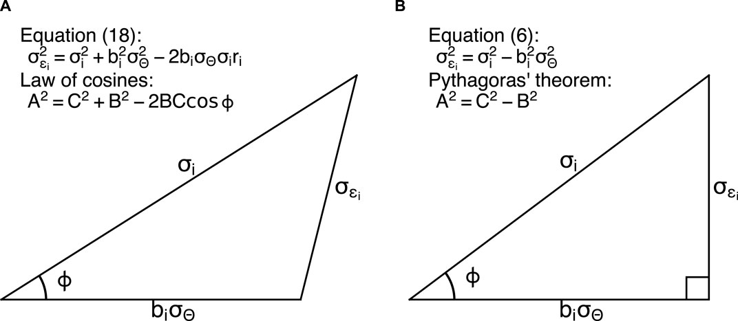
Figure 1. Geometrical meanings of (A) Eq. 18 and (B) Eq. 6. The error standard deviation
We emphasize that all datasets are assumed to be positively correlated with the ground truth in Eqs 10–12, i.e., taking the positive root. Therefore,
The original error variance Eq. 6 resembles the Pythagoras’ theorem (Figure 1B), a special case of the law of cosines. Therefore, the angle between
To summarize, the alternative error variance equation incorporates correlation coefficient, which is absent in the original equation. The new equation forms the basis of the proposed triple collocation diagram.
To demonstrate applications of the new triple collocation diagram, we focus on a measurement related to the abundance of aerosol particles. Aerosols are highly variable in space and time leading to high uncertainty in estimating total anthropogenic radiative forcing (Forster et al., 2021). Three aerosol optical depth (AOD) retrieval datasets are used in this study. AOD quantifies the column-integrated aerosol loading, but more specifically the sum of light scattering and absorption by aerosols (Seinfeld and Pandis, 2006).
Two of the retrievals come from the Aerosol Cloud meTeorology Interactions oVer the western ATlantic Experiment (ACTIVATE) which is one of the National Aeronautics and Space Administration (NASA) Earth Venture Suborbital-3 (EVS-3) missions (Sorooshian et al., 2019; Sorooshian et al., 2023). During ACTIVATE, two NASA Langley Research Center aircraft, the low-flying HU-25 Falcon and high-flying King Air, were strategically deployed to collect in-situ and remotely-sensed measurements over the western North Atlantic Ocean. From February 2020 to June 2022, 174 and 168 flights were successfully completed by the King Air and Falcon, respectively. Among these, 162 were joint flights. AOD was retrieved by two remote sensing instruments onboard the King Air, the Research Scanning Polarimeter (RSP) (Cairns et al., 1999; Cairns et al., 2003) and Second Generation High Spectral Resolution Lidar (HSRL-2) (Hair et al., 2008). The third retrieval comes from the Moderate Resolution Imaging Spectroradiometer (MODIS). Two MODIS sensors have been onboard the Terra and Aqua satellites since 1999 and 2002, respectively. The two satellites observe the Earth along a sun-synchronous orbit at an altitude of around 700 km with a period of 99 min, providing MODIS data at three nadir spatial resolutions (Remer et al., 2005; Levy et al., 2013).
We compare AOD at 532 nm from the three retrievals. For RSP, the aerosol properties are retrieved using the Microphysical Aerosol Properties from Polarimetry (MAPP) algorithm (Stamnes et al., 2018), which then become part of the level 2 aerosol product. For HSRL-2, AOD is derived using extinction coefficients from the difference in molecular return signals (Hair et al., 2008). The original 1-km level 2 RSP and HSRL-2 AOD data are horizontally averaged to a spatial resolution of 3 km, which results in 6,988 pairs. For MODIS, we use the MODIS Collection 6.1 level 2 3-km aerosol product for both satellites: MOD04_3K from Terra and MYD04_3K from Aqua. This product is entirely retrieved using the Dark Target (DT) algorithm (Remer et al., 2013). The native MODIS AOD at 550 nm is converted to 532 nm using the Ångström exponent calculated from the MODIS AOD at 470 nm and 550 nm. For each pair of RSP and HSRL-2 data, we collocate the nearest MODIS data point within
Based on the alternative error variance Eq. 18, a triple collocation diagram is designed to display multiple aspects of triple collocation analysis. A prototype is shown in Figure 2 with three AOD datasets: RSP, HSRL-2, and MODIS. For comparison, an additional figure (see Supplementary Figure S1) is prepared to display the same information using the traditional multi-panel method.

Figure 2. A sample diagram for displaying performance metrics of triple collocation analysis. Three colors represent three different 532-nm AOD datasets during ACTIVATE: RSP (blue), HSRL-2 (red), and MODIS (orange). Three open circles are drawn for each dataset. The radial distance between the origin and the circle on the polar grid is the total (system) standard deviation
For those who are familiar with Taylor diagram, it is straightforward to use the schematic from Figure 1 to recognize the three standard deviation terms and correlation coefficient in Figure 2. The circles on the polar grid represents the total standard deviation. The projections of the total standard deviation on the
During ACTIVATE, HSRL-2 has the smallest error standard deviation
Other metrics can also be easily estimated or computed from the diagram. The values of total standard deviation can be computed using
The triple collocation diagram is not limited to handling three datasets only. For example, seeing that RSP exhibits the largest errors among three datasets (Figure 2), a simple data quality flag is devised to filter out data points with inferior retrievals based on a performance cost function in the RSP retrieval algorithm (Stamnes et al., 2018). Around 50% of triplets are filtered out, and the difference before and after applying the quality flag is shown in Figure 3. Filtered datasets are indicated by squares without changing the color theme. Colored arrows have also been added to follow the changes in performance metrics. Appreciable improvement is seen with RSP data after filtering as the correlation coefficient rises to 0.84 and error standard deviation falls to 0.044 (or a 31% decrease). Note also that if the correlation coefficient increases with the direction of the arrow, the signal-to-noise ratio also increases. An additional figure (see Supplementary Figure S2) is prepared to display the same information using the traditional multi-panel method.

Figure 3. Same as Figure 2 but adding the three datasets after applying an RSP data filter. The three original and filtered datasets are indicated by circles and squares, respectively. Colored arrows indicate the changes from original to filtered datasets.
While various performance metrics have been developed for the triple collocation analysis, it is beneficial to summarize the different aspects of the performance in a single measure. Similar problems have led to the development of skill scores such as Brier skill score and ranked probability skill score in weather and climate prediction (Wilks, 2011) and efficiencies such as Nash–Sutcliffe efficiency and Kling–Gupta efficiency in hydrology. For triple collocation, we propose a skill score,
where
The same datasets in Figure 3 are shown in Figure 4, which is contoured with the proposed skill score (Eq. 19). Before filtering, HSRL-2 owns the highest skill score; after filtering, RSP gains
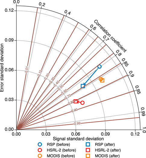
Figure 4. Same as Figure 3 but is contoured with a triple collocation skill score in brown.
The utility of displaying multiple performance metrics in the triple collocation diagram deserves some discussion. The ACTIVATE field campaign provides a rare opportunity to validate the aerosol measurements from two airborne remote sensing instruments on the same platform. The common approach is to compare with Sun photometer measurements from the Aerosol Robotic Network (AERONET) but this is not feasible in our case because no AERONET site is available in the remote ocean over the study region. To get around this issue, we added one more independent satellite dataset and proceeded with the triple collocation analysis.
In the process, we got to be aware of the diverse applications in the literature and the development of various performance metrics. For example,
Triple collocation is a statistical technique that considers three collocated datasets of any geophysical variable and estimates the error characteristics of each dataset without assuming any of the three datasets represent ground truth. Triple collocation analysis involves reporting several performance metrics which can at times become cumbersome using traditional ways of presentation such as multiple-panel plots and long tables.
An alternative equation is derived for the error variance which forms the basis of the proposed triple collocation diagram as a visual aid for condensing multiple aspects of the triple collocation analysis into a two-dimensional polar plot. An observational-based skill score is also obtained to compare performance of three datasets by considering both error variance and correlation coefficient. Three potential applications of the diagram, as illustrated in Figures 2–4, are showcased and discussed. The Taylor diagram has been used to compare the performance of multiple models with an observational-based reference dataset. The proposed diagram complements the Taylor diagram by comparing the performance of multiple observational-based datasets. For interested readers, a routine to draw the triple collocation diagram with several examples is available (see Data Availability Statement).
All the data used in this work are publicly available. The ACTIVATE data can be downloaded from https://asdc.larc.nasa.gov/project/ACTIVATE (NASA/LARC/SD/ASDC, 2021). The MODIS Terra and Aqua data can be downloaded from https://doi.org/10.5067/MODIS/MOD04_3K.061 (MODIS Science Team, 2017b) and https://doi.org/10.5067/MODIS/MYD04_3K.061 (MODIS Science Team, 2017a). The code repository for this work is at https://github.com/leongwaisiu. Further inquiries can be directed to the corresponding author.
LWS: Conceptualization, Data curation, Formal Analysis, Investigation, Methodology, Software, Validation, Visualization, Writing–original draft, Writing–review and editing. XZ: Conceptualization, Funding acquisition, Methodology, Project administration, Resources, Supervision, Writing–review and editing, Data curation, Formal Analysis, Investigation, Software, Validation, Visualization. AS: Conceptualization, Funding acquisition, Methodology, Project administration, Resources, Supervision, Writing–review and editing, Data curation, Formal Analysis, Investigation, Software, Validation, Visualization. BC: Data curation, Formal Analysis, Investigation, Software, Validation, Visualization, Writing–review and editing. CAH: Data curation, Formal Analysis, Investigation, Software, Validation, Visualization, Writing–review and editing. DP: Data curation, Formal Analysis, Investigation, Software, Validation, Visualization, Writing–review and editing. JSS: Data curation, Formal Analysis, Investigation, Software, Validation, Visualization, Writing–review and editing. RAF: Data curation, Formal Analysis, Funding acquisition, Investigation, Resources, Software, Validation, Visualization, Writing–review and editing. JWH: Data curation, Formal Analysis, Funding acquisition, Investigation, Resources, Software, Validation, Visualization, Writing–review and editing.
The author(s) declare that financial support was received for the research, authorship, and/or publication of this article. This work is supported by NASA grant 80NSSC19K0442 for ACTIVATE, a NASA Earth Venture Suborbital-3 (EVS-3) investigation, which is funded by NASA’s Earth Science Division and managed through the Earth System Science Pathfinder Program Office.
We thank the pilots and aircraft maintenance personnel of NASA Langley Research Services Directorate for their work in conducting the ACTIVATE flights. Comments from two reviewers led to an improvement in presentation. We thank Karl Taylor for his comments on an earlier version of the manuscript.
Author DP was employed by Analytical Mechanics Associates Inc.
The remaining authors declare that the research was conducted in the absence of any commercial or financial relationships that could be construed as a potential conflict of interest.
Authors BC, RAF, and DP declared that they were an editorial board member of Frontiers, at the time of submission. This had no impact on the peer review process and the final decision.
All claims expressed in this article are solely those of the authors and do not necessarily represent those of their affiliated organizations, or those of the publisher, the editors and the reviewers. Any product that may be evaluated in this article, or claim that may be made by its manufacturer, is not guaranteed or endorsed by the publisher.
The Supplementary Material for this article can be found online at: https://www.frontiersin.org/articles/10.3389/frsen.2024.1395442/full#supplementary-material
Atlas, R. (1997). Atmospheric observations and experiments to assess their usefulness in data assimilation (gtSpecial IssueltData assimilation in meteology and oceanography: theory and practice). J. Meteorological Soc. Jpn. Ser. II 75, 111–130. doi:10.2151/jmsj1965.75.1B_111
Bluestein, H. B., Carr, F. H., and Goodman, S. J. (2022). Atmospheric observations of weather and climate. Atmosphere-Ocean 60, 149–187. doi:10.1080/07055900.2022.2082369
Cairns, B., Russell, E. E., LaVeigne, J. D., and Tennant, P. M. W. (2003). “Research Scanning Polarimeter and airborne usage for remote sensing of aerosols,” in Proceedings of SPIE. Editors J. A. Shaw, and J. S. Tyo (Bellingham, WA: SPIE), 5158, 33–44. doi:10.1117/12.518320
Cairns, B., Russell, E. E., and Travis, L. D. (1999). “Research Scanning Polarimeter: calibration and ground-based measurements,” in Proceedings of SPIE. Editors D. H. Goldstein, and D. B. Chenault (Denver, CO: SPIE), 3754, 186–196. doi:10.1117/12.366329
Chylek, P., Henderson, B., and Mishchenko, M. (2003). Aerosol radiative forcing and the accuracy of satellite aerosol optical depth retrieval. J. Geophys. Res. Atmos. 108, 1–8. doi:10.1029/2003jd004044
Crutzen, P. J., and Ramanathan, V. (2000). The ascent of atmospheric sciences. Science 290, 299–304. doi:10.1126/science.290.5490.299
Dekking, F. M., Kraaikamp, C., Lopuhaä, H. P., and Meester, L. E. (2005). A modern introduction to probability and statistics: understanding why and how. London, UK: Springer-Verlag.
Deng, X., Zhu, L., Wang, H., Zhang, X., Tong, C., Li, S., et al. (2023). Triple collocation analysis and in situ validation of the CYGNSS soil moisture product. IEEE J. Sel. Top. Appl. Earth Observations Remote Sens. 16, 1883–1899. doi:10.1109/JSTARS.2023.3235111
Dorigo, W. A., Scipal, K., Parinussa, R. M., Liu, Y. Y., Wagner, W., de Jeu, R. A. M., et al. (2010). Error characterisation of global active and passive microwave soil moisture datasets. Hydrology Earth Syst. Sci. 14, 2605–2616. doi:10.5194/hess-14-2605-2010
Draper, C., Reichle, R., de Jeu, R., Naeimi, V., Parinussa, R., and Wagner, W. (2013). Estimating root mean square errors in remotely sensed soil moisture over continental scale domains. Remote Sens. Environ. 137, 288–298. doi:10.1016/j.rse.2013.06.013
Fang, H., Wei, S., Jiang, C., and Scipal, K. (2012). Theoretical uncertainty analysis of global MODIS, CYCLOPES, and GLOBCARBON LAI products using a triple collocation method. Remote Sens. Environ. 124, 610–621. doi:10.1016/j.rse.2012.06.013
Forster, P., Storelvmo, T., Armour, K., Collins, W., Dufresne, J.-L., Frame, D., et al. (2021). “The earth’s energy budget, climate feedbacks, and climate sensitivity,” in Climate change 2021: the physical science basis. Contribution of working group I to the sixth assessment report of the intergovernmental panel on climate change. Editors V. Masson-Delmotte, P. Zhai, A. Pirani, S. Connors, C. Péan, S. Bergeret al. (Cambridge, United Kingdom and New York, NY, USA: Cambridge University Press), 923–1054. doi:10.1017/9781009157896.009
Fu, G., Hasekamp, O., Rietjens, J., Smit, M., Di Noia, A., Cairns, B., et al. (2020). Aerosol retrievals from different polarimeters during the acepol campaign using a common retrieval algorithm. Atmos. Meas. Tech. 13, 553–573. doi:10.5194/amt-13-553-2020
Gruber, A., De Lannoy, G., Albergel, C., Al-Yaari, A., Brocca, L., Calvet, J.-C., et al. (2020). Validation practices for satellite soil moisture retrievals: what are (the) errors? Remote Sens. Environ. 244, 111806. doi:10.1016/j.rse.2020.111806
Gruber, A., Su, C.-H., Zwieback, S., Crow, W., Dorigo, W., and Wagner, W. (2016). Recent advances in (soil moisture) triple collocation analysis. Int. J. Appl. Earth Observation Geoinformation 45, 200–211. doi:10.1016/j.jag.2015.09.002
Hair, J. W., Hostetler, C. A., Cook, A. L., Harper, D. B., Ferrare, R. A., Mack, T. L., et al. (2008). Airborne high spectral resolution lidar for profiling aerosol optical properties. Appl. Opt. 47, 6734. doi:10.1364/ao.47.006734
Hansen, J., Rossow, W., Carlson, B., Lacis, A., Travis, L., Del Genio, A., et al. (1995). Low-cost long-term monitoring of global climate forcings and feedbacks. Clim. Change 31, 247–271. doi:10.1007/BF01095149
Koh, T., Wang, S., and Bhatt, B. C. (2012). A diagnostic suite to assess NWP performance. J. Geophys. Res. Atmos. 117, 1–20. doi:10.1029/2011jd017103
Levy, R. C., Mattoo, S., Munchak, L. A., Remer, L. A., Sayer, A. M., Patadia, F., et al. (2013). The Collection 6 MODIS aerosol products over land and ocean. Atmos. Meas. Tech. 6, 2989–3034. doi:10.5194/amt-6-2989-2013
McColl, K. A., Vogelzang, J., Konings, A. G., Entekhabi, D., Piles, M., and Stoffelen, A. (2014). Extended triple collocation: estimating errors and correlation coefficients with respect to an unknown target. Geophys. Res. Lett. 41, 6229–6236. doi:10.1002/2014gl061322
Mishchenko, M. I., Cairns, B., Hansen, J. E., Travis, L. D., Burg, R., Kaufman, Y. J., et al. (2004). Monitoring of aerosol forcing of climate from space: analysis of measurement requirements. J. Quantitative Spectrosc. Radiat. Transf. 88, 149–161. doi:10.1016/j.jqsrt.2004.03.030
NASA (2021). Aerosol Cloud meTeorology Interactions oVer the western ATlantic experiment (ACTIVATE). doi:10.5067/SUBORBITAL/ACTIVATE/DATA001
O’Carroll, A. G., Eyre, J. R., and Saunders, R. W. (2008). Three-way error analysis between AATSR, AMSR-E, and in situ sea surface temperature observations. J. Atmos. Ocean. Technol. 25, 1197–1207. doi:10.1175/2007jtecho542.1
Remer, L. A., Kaufman, Y. J., Tanré, D., Mattoo, S., Chu, D. A., Martins, J. V., et al. (2005). The MODIS aerosol algorithm, products, and validation. J. Atmos. Sci. 62, 947–973. doi:10.1175/jas3385.1
Remer, L. A., Mattoo, S., Levy, R. C., and Munchak, L. A. (2013). MODIS 3 km aerosol product: algorithm and global perspective. Atmos. Meas. Tech. 6, 1829–1844. doi:10.5194/amt-6-1829-2013
Rodgers, J. L., and Nicewander, W. A. (1988). Thirteen ways to look at the correlation coefficient. Am. Statistician 42, 59–66. doi:10.1080/00031305.1988.10475524
Seinfeld, J. H., and Pandis, S. N. (2006). Atmospheric chemistry and physics: from Air pollution to climate change. 2nd edn. Hoboken, New Jersey: John Wiley & Sons, Inc.
Shinozuka, Y., Johnson, R. R., Flynn, C. J., Russell, P. B., Schmid, B., Redemann, J., et al. (2013). Hyperspectral aerosol optical depths from TCAP flights. J. Geophys. Res. Atmos. 118 (12), 180–212. doi:10.1002/2013jd020596
Sorooshian, A., Alexandrov, M. D., Bell, A. D., Bennett, R., Betito, G., Burton, S. P., et al. (2023). Spatially coordinated airborne data and complementary products for aerosol, gas, cloud, and meteorological studies: the NASA ACTIVATE dataset. Earth Syst. Sci. Data 15, 3419–3472. doi:10.5194/essd-15-3419-2023
Sorooshian, A., Anderson, B., Bauer, S. E., Braun, R. A., Cairns, B., Crosbie, E., et al. (2019). Aerosol–cloud–meteorology interaction airborne field investigations: using lessons learned from the U.S. West Coast in the design of ACTIVATE off the U.S. East Coast. Bull. Am. Meteorological Soc. 100, 1511–1528. doi:10.1175/bams-d-18-0100.1
Stamnes, S., Hostetler, C., Ferrare, R., Burton, S., Liu, X., Hair, J., et al. (2018). Simultaneous polarimeter retrievals of microphysical aerosol and ocean color parameters from the “MAPP” algorithm with comparison to high-spectral-resolution lidar aerosol and ocean products. Appl. Opt. 57, 2394. doi:10.1364/ao.57.002394
Stith, J. L., Baumgardner, D., Haggerty, J., Hardesty, R. M., Lee, W.-C., Lenschow, D., et al. (2018). 100 years of progress in atmospheric observing systems. Meteorol. Monogr. 59 (2), 2.1–2.55. doi:10.1175/amsmonographs-d-18-0006.1
Stoffelen, A. (1998). Toward the true near-surface wind speed: error modeling and calibration using triple collocation. J. Geophys. Res. Oceans 103, 7755–7766. doi:10.1029/97jc03180
Su, C.-H., Ryu, D., Crow, W. T., and Western, A. W. (2014). Beyond triple collocation: applications to soil moisture monitoring. J. Geophys. Res. Atmos. 119, 6419–6439. doi:10.1002/2013jd021043
Taylor, K. E. (2001). Summarizing multiple aspects of model performance in a single diagram. J. Geophys. Res. Atmos. 106, 7183–7192. doi:10.1029/2000jd900719
Thomson, R. E., and Emery, W. J. (2014). Data analysis methods in physical oceanography. 3rd edn. Amsterdam, Netherlands: Elsevier.
Tsamalis, C. (2022). Clarifications on the equations and the sample number in triple collocation analysis using SST observations. Remote Sens. Environ. 272, 112936. doi:10.1016/j.rse.2022.112936
Wilks, D. S. (2011). Statistical methods in the atmospehric sciences. 3rd edn. San Diego, California: Academic Press.
Yilmaz, M. T., and Crow, W. T. (2014). Evaluation of assumptions in soil moisture triple collocation analysis. J. Hydrometeorol. 15, 1293–1302. doi:10.1175/jhm-d-13-0158.1
Keywords: triple collocation, ACTIVATE, RSP, HSRL-2, polarimeter, lidar, MODIS, aerosol
Citation: Siu LW, Zeng X, Sorooshian A, Cairns B, Ferrare RA, Hair JW, Hostetler CA, Painemal D and Schlosser JS (2024) Summarizing multiple aspects of triple collocation analysis in a single diagram. Front. Remote Sens. 5:1395442. doi: 10.3389/frsen.2024.1395442
Received: 03 March 2024; Accepted: 12 June 2024;
Published: 16 July 2024.
Edited by:
Danfeng Hong, Chinese Academy of Sciences (CAS), ChinaReviewed by:
Chun-Hsu Su, Bureau of Meteorology, AustraliaCopyright © 2024 Siu, Zeng, Sorooshian, Cairns, Ferrare, Hair, Hostetler, Painemal and Schlosser. This is an open-access article distributed under the terms of the Creative Commons Attribution License (CC BY). The use, distribution or reproduction in other forums is permitted, provided the original author(s) and the copyright owner(s) are credited and that the original publication in this journal is cited, in accordance with accepted academic practice. No use, distribution or reproduction is permitted which does not comply with these terms.
*Correspondence: Leong Wai Siu, bGVvbmd3YWlzaXVAYXJpem9uYS5lZHU=
Disclaimer: All claims expressed in this article are solely those of the authors and do not necessarily represent those of their affiliated organizations, or those of the publisher, the editors and the reviewers. Any product that may be evaluated in this article or claim that may be made by its manufacturer is not guaranteed or endorsed by the publisher.
Research integrity at Frontiers
Learn more about the work of our research integrity team to safeguard the quality of each article we publish.