Generating hyperspectral reference measurements for surface reflectance from the LANDHYPERNET and WATERHYPERNET networks

The LANDHYPERNET and WATERHYPERNET networks (which together make up the HYPERNETS network) consist of a set of autonomous hyperspectral spectroradiometers (HYPSTAR^®) acquiring fiducial reference measurements of surface reflectance at various sites covering a wide range of surface types (both land and water) for use in satellite Earth observation validation and remote sensing applications. This paper describes the processing algorithm for the HYPSTAR^® data products. The hypernets_processor is a Python software package to process the LANDHYPERNET and WATERHYPERNET in-situ hyperspectral raw data, collected from the measurement network under the standard measurement protocols, to the designated products, through data transmission and conversion, application of calibration, evaluation of reflectance and other variables, and, archiving for distribution to users. In order to achieve fiducial reference measurement quality, uncertainties are propagated through each step of the processing chain, taking into account temporal and spectral error-covariance. Such detailed uncertainty information is unique for any satellite validation network. We also describe the HYPSTAR^® products acquired until 2023–04–31, consisting of 12,190 LANDHYPERNET sequences and 55,514 WATERHYPERNET sequences (of which respectively 11,802 and 44,412 were successfully processed to surface reflectance).

1 Introduction

In recent years, there has been a growing fleet of high-quality optical Earth observation satellite sensors with various spectral bands and/or resolutions. As a result, there is a growing need for high-quality hyperspectral in-situ optical reflectance validation observations, for both land and water. Particularly, the European Space Agency (ESA) has highlighted the need for a network for validating surface reflectance in their Calibration/Validation strategy for optical land-imaging satellites (Niro et al., 2021). There is also an increasing focus on data quality, with the objective to make traceable and uncertainty-quantified measurements, referred to as Fiducial Reference Measurements (FRMs; Goryl et al., 2023).

By moving from mobile measurement setups to the use of autonomous platforms over a variety of surface types, there are many more matchups available for a given satellite. When this is combined with taking hyperspectral measurements and integrating over the satellite spectral response function, the data from a single site can be used to reconstruct the signal for many optical missions (S2, S3, PROBA-V, MODIS, VIIRS, L8, Pléiades, ENMAP, PRISMA, SABIAMAR, PACE, etc.). The existing AERONET-OC (Zibordi et al., 2009; Zibordi et al., 2021) and RadCalNet (Bouvet et al., 2019) networks provide reference in situ measurements, and have been shown to be suitable for performing validation of satellite products (e.g., Alonso et al., 2019; Ishizaka et al., 2022; Zibordi et al., 2022). However both these networks are based on multispectral instruments (with the exception of the Chinese RadCalNet sites), which require spectral interpolation and modelling associated uncertainties to cover all spectral bands of all sensors.

The Horizon 2020 HYPERNETS project set out to meet these needs by developing a network of autonomous field sites for the measurement of high-quality, hyperspectral surface reflectance. To achieve this, a new hyperspectral radiometer, HYPSTAR^® (Hyperspectral Pointable System for Terrestrial and Aquatic Radiometry; Kuusk et al., in this issue), with instrument pointing capabilities has been developed and is currently operational at several land (LANDHYPERNET; Bialek et al., in this issue) and water (WATERHYPERNET; Ruddick et al., in this issue) sites. The data from these new instruments are centrally processed, with consistent processing for water and land reflectances, by the hypernets_processor to radiance, irradiance and reflectance products with associated uncertainties. The HYPERNETS satellite validation network is expected to become the main source of surface reflectance validation data for all spectral bands of VNIR-SWIR optical missions with detailed uncertainty estimates and including error-correlation information. It is the first network with such a detailed metrological approach in terms of uncertainty analysis.

The hypernets_processor is the network processor to handle both water and land data from HYPSTAR^® acquisitions through transmission, conversion, application of calibration, interpolation, evaluation of reflectance and other products and archiving for web distribution. Quality control is performed at different stages throughout the processing. The data are managed in line with the Findable, Accessible, Interoperable and Re-useable (FAIR) principles of data management (Wilkinson et al., 2016). Measurement and calibration uncertainty is propagated through the full processing chain, including treatment of temporal and wavelength error-covariance following a metrological approach as defined in the Guide to the Expression of Uncertainty in Measurement (JCGM 100:2008, 2008). These data are now publicly available as part of the WATERHYPERNET and LANDHYPERNET network respectively.

This paper presents the reference description of the v2.0 of the hypernets_processor and its products. Previously, a summarised description of a beta version of the hypernets_processor was presented in Goyens et al. (2021). In Section 2, some information on the HYPERNETS project and HYPSTAR^® instrument are summarised. Section 3 details the processing algorithms used, including the different steps used as well as the different quality checks and the uncertainty propagation. In Section 4, the different data products produced by the hypernets_processor and their distribution are described. In Section 5, some examples and processing statistics are provided. Section 6 lists some of the improvements that are foreseen in the near future. Finally, Section 7 provides the conclusions.

2 HYPERNETS

2.1 HYPSTAR^® instrument

HYPSTAR^® (Hyperspectral Pointable System for Terrestrial and Aquatic Radiometry; www.hypstar.eu) is an autonomous hyperspectral radiometer system dedicated to surface reflectance validation of all optical Copernicus satellite data products. For a complete description of the HYPSTAR^® system, we refer to Kuusk et al. (in this issue). HYPSTAR^® takes radiance and irradiance measurements using the same spectrometer (though with different optical paths for radiance and irradiance). Two slightly different instruments are used for water and land: (1) The Standard Range (SR) model provides visible and near-infrared (VNIR, 380–1,020 nm) data and is used on water sites, (2) the eXtended Range (XR) models have an additional shortwave-infrared (SWIR) spectrometer module which extends the spectral range up to 1680 nm. The XR models are meant to be used on the land sites. Pictures of the SR and XR models of the HYPSTAR^® are shown in Figure 1, together with some example field sites. The instrument characteristics are summarised in Table 1.

Figure 1

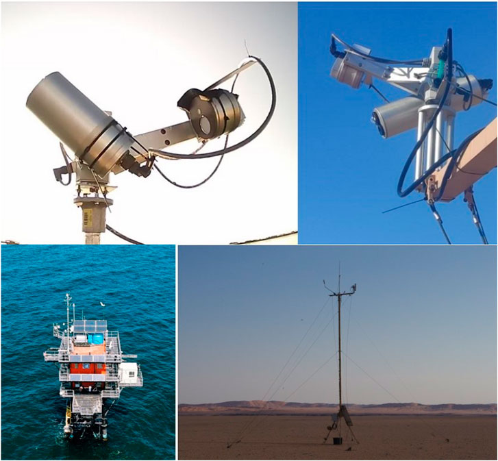
Figure 1. Picture of the Standard Range (SR) HYPSTAR^® system (including validation module) used for the WATERHYPERNET network (top left) and the eXtended Range (XR) HYPSTAR^® system (including validation module) used for the LANDHYPERNET network (top right). A picture of one of the water sites (Aqua Alta, bottom left) and one of the land sites (Gobabeb, bottom right) is also shown.

Table 1

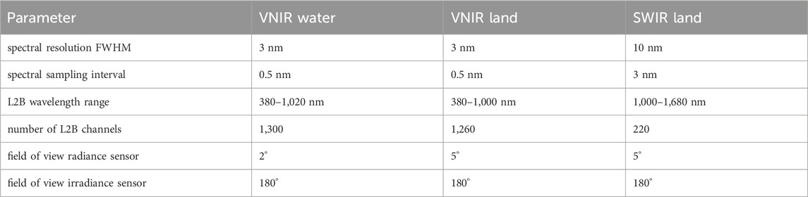
Table 1. Instrument characteristics for the water HYPSTAR^® (SR model) and land HYPSTAR^® (XR model, consisting of VNIR and SWIR module) sensors. All values in the table are approximate values. Precise values might be slightly different and vary from instrument to instrument.

The spectral sampling of the HYPSTAR^® is 0.5 nm in the VNIR and 3 nm in the SWIR, and the spectral resolution full-width half-maximum (FWHM) is 3 nm in the VNIR and 10 nm in the SWIR. The SWIR sensor is actively cooled (typically to 0 °C, but this can be configured) to ensure the stability of the measurements. The field of view of the radiance measurements is $\sim 2°$ for the SR model and $\sim 5°$ for the XR model. The irradiance measurements observe the full hemisphere, i.e. 180°. The HYPSTAR^® system is mounted on a low-cost pointing system which allows the acquisition of autonomous, multi-angular measurements. A GPS, light and rain sensors as well as cameras to image the target and the sensor heads are also included. Data acquired by the HYPSTAR^® is saved in separate binary ‘.spe’ files for each viewing geometry. These acquisitions are sent to the central server for processing, together with some ‘rgb’ images taken by the camera within the system, a file with meteorological information (i.e., relative humidity, temperature and pressure measured within the system and illuminance measured by an external light sensor), log files made during the acquisition and data transfer, and a metadata file.

The HYPSTAR instruments are calibrated by Tartu University¹ (See Kuusk et al. in this issue). Currently this includes radiometric calibration (gains) and non-linearity calibration (non-linearity coefficients). Measurements of the temperature responsivity and stray light are also planned/in progress, but these characterisations are not yet used in the processing of the data in the current processor version. The lab calibration also includes a wavelength calibration. The wavelengths for each instrument will thus be slightly different, and the radiance and irradiance measurements can also have slightly different wavelengths for each spectral pixel (see Section 3.2.4.1). The wavelength calibration assigns a wavelength to each spectral pixel in the raw data, but not all the raw data pixels will be used in the final product. This is either because these wavelengths (e.g., in the UV) cannot be calibrated due to the spectral limits of the radiometric calibration references used, or because these wavelengths are simply too noisy to be used. In the final publicly distributed data (L2B products) the wavelength range is limited to the ranges specified in Table 1 in order to only supply the user with the best quality data.

2.2 HYPERNETS measurement protocol and terminology

Radiometer measurements are taken in a defined set of geometries called a sequence. For the WATERHYPERNET network, the output of a single sequence is the resulting water-leaving reflectance (possibly measured at different relative azimuth angles between Sun and sensor) and associated uncertainty and quality flags. For the LANDHYPERNET network, it is a set of surface reflectance measurements for different viewing geometries with associated uncertainties and quality flags. The set of acquisitions at each viewing geometry in a sequence is called a series, and it is composed of a set of repeat measurements called scans (which will be averaged). Hence, one scan results in a single unique spectrum with a specific integration time. The number of repeat scans in a single series depends on the desired parameter and its natural variability, potentially constrained by the total duration and power consumption. For the land XR instruments, the SWIR sensors typically have larger integration times than the VNIR sensors (in order to optimally use the dynamic range of the sensor). Typically, a fixed number (the default is 10) of SWIR scans will be set, and the VNIR sensor will keep taking scans until the SWIR sensor has completed its scans (leading to a larger number of scans for VNIR than for SWIR).

The geometries for the HYPERNETS network are defined in Figure 2. Each of the angles are defined in the reference frame centred on the measurement location on the surface. The viewing angles are thus defined as the sensor ‘viewing from’ a particular direction. In the side view, the viewing zenith angles are computed from Nadir to Zenith, i.e., a viewing zenith angle, θ_v, of 180° is looking upward (e.g., for downwelling irradiance measurements). The solar zenith angle is measured from Zenith. In the top view, the viewing azimuth angle, φ_v, is the angle measured clockwise from the absolute North to the direction of the sensor (i.e., the line from the target to the sensor). This definition of the viewing azimuth angle matches that of most optical satellite geometries (such as those of Sentinel-2, Sentinel-3, Landsat 8). Two additional azimuth angles are defined, i.e., the ‘pointing-to’ azimuth angle, φ_p, measured clockwise from the absolute North to the pointing direction (i.e., the line from the sensor to the target, or, φ_v+180°), and, the relative azimuth angle, Δφ, measured clockwise from the Sun to the pointing direction (i.e., φ_p-φ_s). In this definition, Δφ = 0 means the instrument is looking towards the Sun, and Δφ = 180 means the instrument is looking away from the Sun. Our definitions of φ_p and Δφ match the definitions in Ruddick et al. (2019) for their viewing azimuth and Δφ, respectively (see their Figure 1).

Figure 2

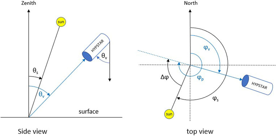
Figure 2. Left: Side-view diagram defining viewing zenith angles θ_v and solar zenith angles θ_s. Right: Top-view diagram defining the viewing azimuth angles φ_v, ‘pointing-to’ azimuth angle φ_p and solar azimuth angles φ_s, measured clockwise from North. The relative azimuth angle Δφ is defined as the difference between φ_p and φ_s. All angles are defined in the reference frame centred on the measurement location on the surface.

Figure 3 illustrates the measurement protocol for a WATERHYPERNET sequence. The current standard water protocol follows commonly used measurement protocols (Ruddick et al., 2019, and references therein). Upwelling above-water radiance, L_u, series are taken at θ_v = 40° and sun-sensor relative azimuths, Δφ, at ± 90° and/or ± 135° (to avoid Sun glint and high skylight reflectance within the sensor field of view). Each series of L_u is preceded and followed by a series of above-water downwelling (sky) radiance, L_d, in the specular reflection direction for the correction of the reflected skylight (i.e., θ_v for L_u = 180° - θ_v for L_d). Downwelling irradiance, E_d, series are taken at the beginning and the end of each sequence. A standard water sequence (including only one single azimuth angle) lasts approximately 5 min and is executed every 15–30 min during daylight.

Figure 3

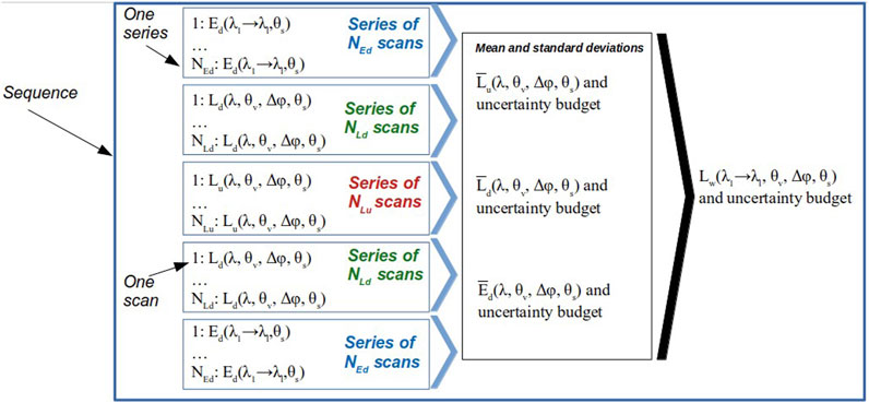
Figure 3. Diagram illustrating the measurement protocol for the WATERHYPERNET network with a sequence being a series of scans of upwelling radiance L_u preceded and followed by a series of scans of downwelling irradiance, E_d, and a series of scans of downwelling radiance L_d. In the figure N_x, λ, θ_v, θ_s, and, Δϕ stand for number of scans, wavelength, viewing zenith angle, solar zenith angle and relative azimuth angle, respectively.

The LANDHYPERNET sequences also start and end with downwelling irradiance series, but have multiple upwelling radiance series covering a range of different viewing geometries (including a minimum of five view zenith and six view azimuth angles). The design of the land measurement protocol aims to optimise the viewing geometry during satellite’s overpass times and by its repeats through the day to obtain information about Bidirectional Reflectance Distribution Function (BRDF) properties of the site. A plot illustrating the different viewing geometries for a land sequence is illustrated in Figure 4. Land sequences do not measure the downwelling (sky) radiance. A standard land sequence typically lasts approximately 15 min (depending on illumination) and is executed every 30 min during daylight.

Figure 4

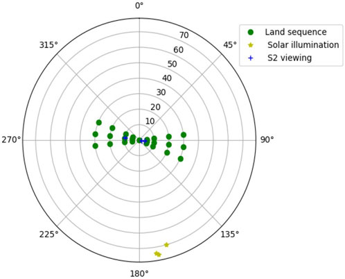
Figure 4. Polar plot showing the typical land protocol viewing geometries for the LANDHYPERNET network. As an example, the Sentinel-2 viewing geometries and solar geometries (during Sentinel-2 overpass) for the NPL Wytham Woods site in January 2022 are shown for comparison.

WATERHYPERNET and LANDHYPERNET sequences following the above protocols are called ‘standard’ sequences.

2.3 Hypernets_processor design

The hypernets_processor module is an open source Python package, with the code actively developed on GitHub². It has a modular design that enables simple development. The various processing steps (described in the next section) have been implemented within a flexible framework, so that rapid advances in instrumentation and systems can be easily accommodated. The software is run through a command-line interface (CLI) and ingests data and processes with 24/7/365 operation including automated monitoring of diagnostics both for the network operator and for the site operators. Installation instructions are available in the hypernets_processor documentation³.

The hypernets_processor has a number of different categories of usage or modes of operation, to provide context to the rest of the design, they are initially described here. The first distinction is between the LANDHYPERNET processor and the WATERHYPERNET processor.

• LANDHYPERNET processor - processing for data taken by the LANDHYPERNET Network.

• WATERHYPERNET processor - processing for data taken by the WATERHYPERNET Network.

Where possible, the processing of the LANDHYPERNET and WATERHYPERNET is done as consistently as possible, with deviations between them only in the L1C and L2A processing (Figure 5). Also, there is a distinction between whether the measured data are from a standard measurement sequence or custom measurement sequence.

• Standard Sequence - dataset containing the standard set of measurements defined by the LANDHYPERNET or WATERHYPERNET network (as described in Section 2.2).

• Custom Sequence - dataset containing any other set of measurements.

Figure 5

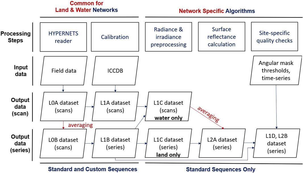
Figure 5. Design diagram for the hypernets_processor. Inputs from raw field acquisitions and the instrument characterisation and calibration database (ICCDB) are processed in various steps to the L0A-L2B HYPERNETS products. The processing steps row indicates what step of the processor has been used to create the output files in that column. The averaging processing step is applied at different stages throughout the processing, as indicated with the red arrows.

Standard sequences are automatically processed to L2A, whereas custom sequences are only processed to L1B (flags and anomalies will be raised, triggering an anomaly that will stop the processing, see Section 3.3). Finally, there is the distinction between the two potential use cases, network processing or field use.

• Network Processing - automated processing to prepare standard sequences retrieved from network sites for distribution to users.

• Field Use - ad hoc processing of particular field acquisitions, for example, for testing instrument operation in the field.

In the remainder of this paper, we will mainly focus on the network processing of standard sequences. For further information on the use case of field use, we refer the reader to the corresponding page in the hypernets_processor documentation⁴.

2.4 Hypernets_processor options

There are many options that can be fine-tuned in the running of the hypernets_processor, from controlling which measurement functions are used, where to store the output data and what plots and output files are produced, to details like number of Monte Carlo iterations used in the uncertainty propagation, thresholds of the quality checks or what ancillary data to use in the calculation of the air-water interface reflection factor (referred to as ‘rhof_option’). These options can be controlled through three config files. The processor.config file contains all the options that are in common between all sites (different processor.config files are used for the WATERHYPERNET and LANDHYPERNET network, though with most values in common). The job.config file controls all site-specific options. Finally, there is also a scheduler.config file which controls how often the hypernets_processor checks for new data and how many sequences can be processed in parallel.

Set up routines are available to set up the processor (and the processor.config file using default values), to set up a new job (i.e., the processing of a new site, including what directory to check for new data) and to start the scheduler. The hypernets_processor documentation provides more information on how to set up and run the automated processing⁵.

2.5 Hypernets_processor versions

The version of the hypernets_processor described in this paper is v2.0. This is the first version that is intended for operational use. Previous versions include a beta version (as described in Goyens et al., 2021), and a v1.0 which was used to produce the first public dataset on Zenodo (see Section 4.4). A new version of the dataset on Zenodo will be released upon publication of this paper, using the v2.0 of the hypernets_processor.

The version number is made up of two numbers. The first indicates the major version number. Changes to this number indicate significant changes and improvements to the code, and major changes to the datafiles. The second number, called the minor version, is incremented when there are minor feature changes or notable fixes which do not significantly change how the data products should be used.

Compared to the v1.0, there are a few changes in the v2.0 hypernets_processor worth noting, so that any HYPERNETS results using the v1.0 data products can be understood.

• The first important difference is in the definition of the viewing azimuth angles, which have changed by 180° in order to be consistent with satellite viewing azimuth angles in v2.0 (see Section 2.2). The pointing azimuth angles in v2.0 are equal to the viewing azimuth angles in v1.0. Pointing azimuth angles are mainly of interest for the WATERHYPERNET network as it is commonly used (Ruddick et al., 2019, and references therein) to compute the relative azimuth angles.

• Uncertainty propagation is now consistently applied to all WATERHYPERNET products, in the same way as for the LANDHYPERNET network.

• Output files and their names have slightly changed, e.g., there are now L0A and L0B files as opposed to only L0 files, and, the relative azimuth angle, used for the approximation of the air-water interface reflection factor within the WATERHYPERNET network, is also added to the L1C and L2A product names.

• Reflectance files with site specific quality checks applied are called L2B files in v2.0 (see Section 3.3.7), as opposed to L2A files in v1.0. These are the main files to be distributed.

• There were many minor changes (e.g., to the metadata and the quality checks) that are not worth noting individually but do make a difference to the produced HYPERNETS products.

3 Processing algorithm

3.1 Processing overview

The network processing is done centrally on the LANDHYPERNET and WATERHYPERNET servers, through a command line interface, which continuously checks for new data, and processes it as soon as it comes in. The hypernets_processor takes the data from acquisition (raw data) to application of calibration and quality controls, computation of correction factors (e.g., air-water interface reflectance correction for water processing), temporal interpolation to coincident timestamps, processing to surface reflectance and averaging per series. A diagram showing the design for the network processing is provided in Figure 5.

The inputs are the raw field acquisitions and the instrument characterisation and calibration database (ICCDB). The main outputs are the various L0A-L2B NetCDF datasets listed in Table 2. The hypernets_processor also produces various plots and SQL databases of successfully processed products and anomalies (Section 4.3). The different processing steps and the plots produced are described in the next section. As part of the processing, quality checks are performed which either add quality flags to the produced data processing, or in some cases raise anomalies and halt the processing. These quality checks are described in Section 3.3. Uncertainties are also propagated through each of the processing steps, as described in Section 3.4. Details on the produced products are provided in Section 4.

Table 2

Table 2. hypernets_processor processing levels.

3.2 Processing steps

3.2.1 HYPERNETS reader

The hypernets_reader module processes the raw dataset (in spe-binary file format) to the L0A data product (readable NetCDF file). It reads the metadata file of the sequence (ASCII file), as well as the spe-binary data file for each series (the different scans are concatenated per series). According to the metadata file and the filename of the spe-binary file, the processing reorders the scans to L0A radiance, irradiance and darks and outputs for each of those a NetCDF with the different scans. The module also copies and renames the RGB images taken from the target and/or the sky during the sequence with the time of acquisition, the series number and the viewing and (relative) azimuth angle.

3.2.2 Calibration

After the raw L0A data has been read in, it needs to be quality checked and calibrated in order to get the radiance and irradiance L1A data products. The first step consists of assigning wavelengths to each of the spectral pixels based on laboratory characterisation measurements (and omitting pixels outside the calibration range). Next, the L0A dark scans are combined with the L0A (ir)radiance files, assigning each dark to the right (ir)radiance series. Next, the quality checks described in Section 3.3.2 are applied. In order to get calibrated (ir)radiances, the calibration coefficients and non-linearity coefficients (as determined by the calibration laboratory at Tartu University⁶) are then applied to the raw data. Figure 6 shows the raw L0A data and the calibrated L1A data for an land sequence example.

Figure 6

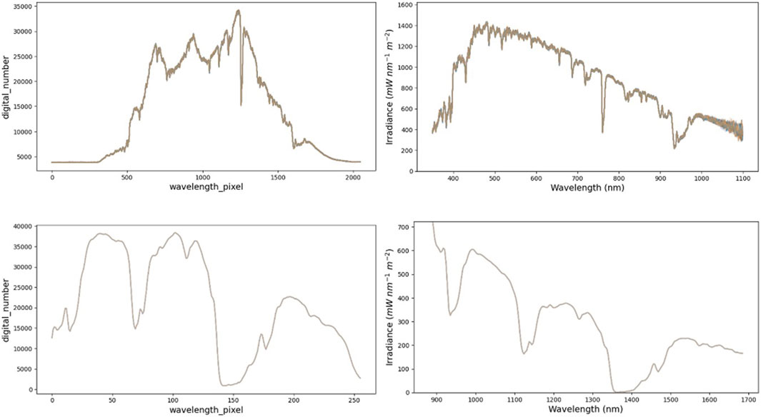
Figure 6. Example of the calibration process for the Gobabeb hyperspectral Namibia site (GHNA) sequence on 2022–10–06 at 9 a.m. UTC. The left panels show the digital numbers (L0A) for the irradiance series at the start of the sequence (all scans plotted) of the VNIR (top) and SWIR (bottom) sensors. The right panels show the calibrated irradiance scans (L1A) of the VNIR (top) and SWIR (bottom) sensors.

When multiple calibration files are available (i.e., at different calibration dates) the one nearest to the acquisition time is used, though only looking backward. When reprocessing data, calibration dates after the acquisition date are thus ignored. Interpolation between pre-deployment and post-deployment calibrations will be explored in the future (see Section 6).

The exact measurement function to be used can be specified manually by providing the measurement function as a standalone Python script. If no custom measurement function is provided, a default measurement function is used. This measurement function is defined by: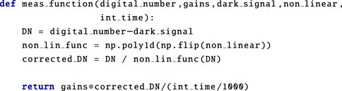

where each of the arguments is a numpy array, digital_number gives the measured signal (in digital numbers), dark_signal gives the dark signal in digital numbers, gains gives the calibration coefficients, non_linear has the polynomial non-linearity coefficients, and int_time is the integration time of the measurement (in ms). An update to this default measurement function is foreseen in a future release, which will include temperature and spectral straylight corrections. The gains and non-linearity coefficients are taken from the most recent calibration data for the given instrument.

The same measurement function is applied for radiance and irradiance measurements, but the gains (as well as the measurements themselves) will be different. Note that the non-linearity coefficients are the same for both radiance and irradiance head (assuming that the non-linearity results from the sensor and internal electronics). For the LANDHYPERNET network, the VNIR and SWIR sensors also both use the same measurement function, and each have their own set of calibration and non-linearity coefficients.

Uncertainties on each of the input quantities (i.e., digital_number, gains, dark_signal, non_linear and int_time) can optionally be propagated to the L1A products using punpy uncertainty propagation package. More details are provided in Section 3.4.

3.2.3 Averaging

In order to get the best averaged results and associated uncertainties per series, the most robust approach is to first average the L0A data (i.e., radiance, irradiance and dark scans in digital numbers). Only the scans that passed the L1A quality checks (see Section 3.3.2) are used in the mean. The averaged raw data make up the L0B datasets. Next, the averaged results in the L0B datasets are calibrated using the same approach as in the previous section.

For the WATERHYPERNET network these calibrated results are directly saved as the L1B datasets, which are an important output of the hypernets_processor as these are made publicly available. for the LANDHYPERNET network, after applying the calibration, the VNIR and SWIR data are combined (for the WATERHYPERNET network no SWIR data are acquired, and this step is skipped). This is done by simply appending all VNIR measurements with wavelengths smaller than 1,000 nm with all SWIR measurements with wavelengths larger than 1,000 nm. The VNIR-SWIR combined, averaged data are then saved as the L1B datasets. An example L1A plot for irradiance is shown in the right panel of Figure 6.

3.2.4 Radiance and irradiance preprocessing

3.2.4.1 LANDHYPERNET network interpolation

The L1C processing for the LANDHYPERNET network consists of two interpolation steps that are applied to the irradiance measurements in order to bring them to the same wavelength scale and timestamps as the radiance measurements.

• Spectral interpolation: The irradiances are spectrally interpolated to the wavelengths of the radiance measurements (which are not identical to the irradiance measurements). Currently, we use a simple linear interpolation.

• Temporal interpolation: Next, we use a similar method to perform a temporal interpolation. In this case, we interpolate the irradiance measurements at the start and end of the sequence, to each of the timestamps of the radiance measurements. A correction is applied to take into account the change in solar zenith angle during the sequence.

The output of the L1C processing is a product with irradiances that now have the same wavelengths and timestamps as the radiance measurements. The radiances in the L1C dataset are unchanged from the L1B dataset. An example of the L1C interpolated irradiances is shown in Figure 7.

Figure 7

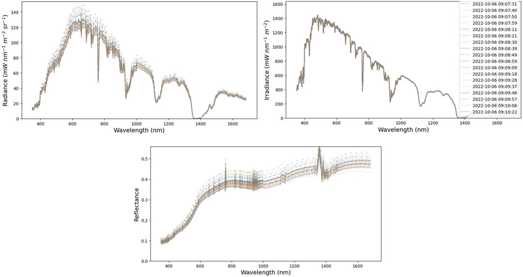
Figure 7. Example of the interpolation and surface reflectance calculation for the GHNA sequence on 2022–10–06 at 9 a.m. UTC. The top left panel shows 45 radiance series (L1B/L1C), which each have a different geometry, and which were acquired one after another. The top right panel shows the irradiance series (L1C), spectrally and temporally interpolated to match the radiance series. The various interpolated lines are very close to each-other. The bottom panel shows the surface reflectances (L2A) calculated using the radiances and irradiances in the L1C dataset.

There are multiple options available for the interpolation. For the temporal interpolation, the default option includes a correction for the change in solar zenith angle throughout the sequence. Prior to the interpolation, the irradiances are divided by the cosine of the solar zenith angle at the time of the irradiance acquisition. After the interpolation, the irradiances are multiplied by the cosine of the solar zenith angle at the timestamps of the radiances. Alternatively, there is also an option to not apply the solar zenith angle correction (i.e., only linear interpolation).

By default, the linear interpolation method is used for both the spectral and temporal interpolations. However, optionally, the hypernets_processor can also be set up to do interpolation following a model. This is done using the interpolation tool within the NPL CoMet toolkit to interpolate between the irradiance wavelengths using a high-resolution reference⁷. The high resolution reference for the spectral irradiance interpolation comes from a clear-sky model, which gives a good first-order approximation of the short scale variability. This model is then scaled to go through the measured irradiance data, while taking into account the spectral response function of the different HYPSTAR^® measurements.

The interpolation option using a high resolution model has been implemented, but is not currently operationally used. Further investigations are required to assess whether these alternative interpolation methods lead to sufficient improvement in the performance to justify their significantly slower runtime.

3.2.4.2 WATERHYPERNET network

The L1C processing for the WATERHYPERNET network consists of multiple steps including (1) water-specific quality checks, (2) temporal and spectral interpolation steps mirroring the land processing, and, (3) computation of the water-leaving radiance and reflectance for each upwelling radiance scan. For the latter, the hypernets_processor uses a water specific processing component, referred to as RHYMER (Reliable processing of HYperspectral MEasurement of Radiance, version on 2020–10–16, written by Quinten Vanhellemont and adapted for the water hypernets_processor by Clémence Goyens).

In its current version, RHYMER provides all the required functions to process above water measurements to water-leaving radiance and water-leaving reflectance (referred hereafter as water reflectance), including the estimation of the air-water interface reflection coefficient using Mobley (1999), Mobley (2015). RHYMER is written such that it can easily be adapted to use alternative look-up-tables, processing functions and/or quality flags. Note that the L1C processing takes as input the L1A files (i.e., not the L1B files as done for the LANDHYPERNET network processing) as it checks for water specific quality flags per upwelling radiance scan. In addition, if the processor encounters measurements made at different relative azimuth angles (and provided that the standard measurement protocol is followed), the processor will estimate the reflectance at each relative azimuth angle Δφ. Therefore, the final dimensions of the L1C data level are wavelength and the number of quality-checked scans of the upwelling radiance measurements. A separate L1C data file is created for each relative azimuth angle.

The L1C radiance and irradiance processing steps are the following.

• Cycle parse: The processor parses through the sequence and verifies, for a single azimuth angle and after applying the required quality checks (see Section 3.3), if the sequence has the required number of downward irradiance (θ_v = 180°) and radiance (θ_v = 140°) scans and corresponding upward radiance scans (θ_v = 40°). If these requirements are not met, the sequence is not further processed and an anomaly is raised (see Section 3.3).

• Spectral interpolation: Likewise for the LANDHYPERNET network processing, the irradiance measurements are spectrally interpolated in order to bring them to the same wavelength scale as the radiance measurements.

• Temporal interpolation: Next, the downwelling radiance and irradiance measurements are averaged per series and each series is temporally interpolated to the same timestamps as the upwelling radiance measurements (including a correction to account for viewing zenith angle, likewise the temporal interpolation of the land processing mentioned above).

• Auxiliary data retrieval: All the required parameters for the computation of the water-leaving radiance and reflectance, i.e., wind speed, ws, and the air-water interface reflection factor, ρ_f (θ_v, θ_s, Δφ, ws), are retrieved. The default wind speed is taken from NCEP/GDAS (National Centers for Environmental Prediction, National Weather Service, NOAA, U.S. Department of Commerce, 2015) and is spatially and temporally interpolated according to the site location and the measurement date and time. Other data sources or a constant value for wind speed can also be used. Based on the retrieved wind speed, ρ_f (θ_v, θ_s, Δφ, ws) can be extracted from different look-up tables, e.g., Mobley (1999) or Mobley (2015). Figure 8 (left panel) shows an example of the estimated reflectance for a single sequence, but for different Δφ (i.e., 225° and 270°) and wind speeds (retrieved from NCEP/GDAS (default) and using a constant value of 2 m⁻¹). The options used for the retrieval of the wind speed and the air water interface reflectance factor can be set in the configuration file (e.g., rhof_option: Mobley1999 and wind_ancillary: GDAS) and are recorded in the metadata of each processed datafile for traceability.

• Retrieval of water-leaving radiance and reflectance: For each L_u scan and from the averaged and temporally interpolated L_d, the water-leaving radiance, L_w, is computed as in Eq. 1 below.

$L_w\left({\theta }_v,\mathrm{\Delta }\phi ,\lambda ,{\theta }_s\right)=L_u\left({\theta }_v,\mathrm{\Delta }\phi ,\lambda ,{\theta }_s\right)-\left[{\rho }_f\left({\theta }_v,\mathrm{\Delta }\phi ,\lambda ,{\theta }_s,ws\right)L_d\left(180-{\theta }_v,\mathrm{\Delta }\phi ,\lambda ,{\theta }_s\right)\right](1)$

The water-leaving radiance is then converted into water reflectance (omitting illumination and viewing dimensions for brevity) in Eq. 2 below using the downwelling (hemispherical) irradiance E_d:

${\rho }_{w,nosc}\left(\lambda \right)=\pi \frac{L_w\left(\lambda \right)}{E_d\left(\lambda \right)}(2)$

with nosc referring to non similarity corrected reflectance. Indeed, although most acquisition protocols attempt to avoid Sun glint, over wind roughened surfaces the target radiance may still contain some Sun glint. Therefore, a spectrally flat correction, ϵ, based on the “near infrared (NIR) similarity spectrum” correction from Ruddick et al. (2006), is applied. The constant ϵ is estimated in Eq. 3 using two wavelengths in the NIR (default for λ₁ and λ₂ are 780 and 870 nm, respectively).

$ϵ\left({\lambda }_1,{\lambda }_2\right)=\frac{\alpha {\rho }_{w,nosc}\left({\lambda }_2\right)-{\rho }_{w,nosc}\left({\lambda }_1\right)}{\alpha -1}(3)$

α is the similarity spectrum ratio for the bands used (the default is, α(780,870) = 1.912). The water reflectance ρ_w is given in Eq. 4 below.

${\rho }_w\left(\lambda \right)={\rho }_{w,nosc}\left(\lambda \right)-ϵ\left({\lambda }_1,{\lambda }_2\right)(4)$

Figure 8 (right panel) shows an example of the estimated reflectance for a single sequence with and without the NIR similarity correction. The data shown in this figure are for the WRUK site, an inland water basin with relatively clear waters. Hence, the NIR similarity correction can be applied (in contrast to turbid water sites such as MAFR or M1BE, see Table 5).

Figure 8

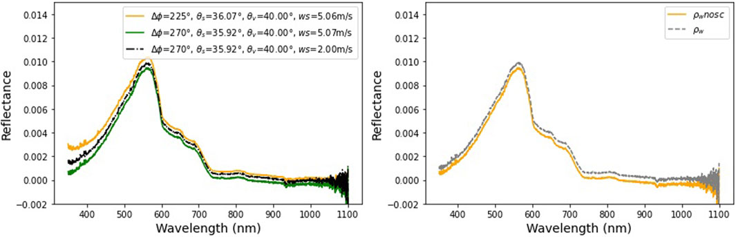
Figure 8. Example of the water-leaving reflectances for the Wraysbury Reservoir, UK site (WRUK) sequence on 2023–07–07 at 1:45 p.m. UTC. The left panel shows reflectance without NIR similarity correction (ρ_w,nosc) for different relative azimuth angles (Δφ equals 225° and 270°, respectively) and wind sources (i.e., retrieved from NCEP/GDAS and default 2 m⁻¹). The right panel shows the reflectance with (ρ_w) and without the NIR similarity correction (ρ_w,nosc).

3.2.5 Surface reflectance calculation

3.2.5.1 LANDHYPERNET network

For the LANDHYPERNET network, the surface reflectances can now be calculated from the L1C radiances, L_u, and irradiances, E_d in Eq. 5 below.

$\rho =\pi \frac{L_u}{E_d}(5)$

We note that this surface reflectance is technically the hemispherical-conical reflectance factor and not the bidirectional reflectance factor, as the contribution from sky reflectance is included in the measurements and the field-of-view of the LANDHYPERNET is 5°.

An example with all the different series is shown in the right panel of Figure 7. In addition, Figure 9 shows additional useful plots produced by the hypernets_processor. This includes plots showing the reflectance variation for a fixed value of viewing azimuth angle (98°) and viewing zenith angle (30°), as well as a polar plot showing the reflectances at 900 nm for each of the included geometries. This shows the smooth variation of the surface reflectance with different angles. In the future, we will investigate whether BRDF models can be fitted to these data (Section 6). These data might in the future be provided as a L2C or L2D dataset.

Figure 9

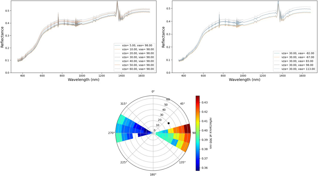
Figure 9. Example of the surface reflectances for the GHNA sequence on 2022–10–06 at 9 a.m. UTC. The top left panel shows the variation with viewing zenith angle for the scans with a viewing azimuth angle of 98°. The top right panel shows the variation with viewing azimuth angle for the scans with a viewing zenith angle of 30°. The bottom panel shows a polar plot with the 900 nm reflectances for each of the different included viewing geometries (zenith angle for radial axis, azimuth angle for angular axis). The solar geometry is shown by the black dot.

3.2.5.2 WATERHYPERNET network

For each L1C data file (one per relative azimuth angle), the surface reflectances and water radiances (computed at each L_u timestamp) are averaged. This results in L2A files containing one spectrum for each variable (i.e., water-leaving radiance, and, water reflectance with and without the NIR similarity correction) and the associated uncertainties. Figure 10 shows an example of the reflectance spectra measured at the WRUK site on 2023–07–07 from the L1C processing level and the averaged L2A reflectance spectrum. Measurements were made at two different relative azimuth angles, i.e., 225° (or −135°) and 270° (or −90°). Hence, as shown in Figure 10, more variability in the L1C reflectance spectra results in higher uncertainties for the L2A reflectance spectrum (see Section 3.4 for more details about uncertainties).

Figure 10

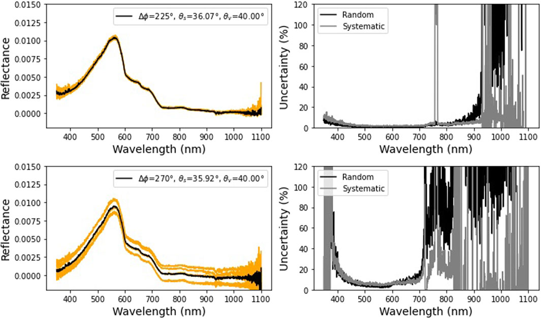
Figure 10. Example of the water-leaving reflectances (without NIR similarity correction (ρ_w,nosc)) for the WRUK sequence on 2023–07–07 at 1:45 p.m. UTC. The left panel shows reflectance of the L1C processing level (orange) together with the averaged L2A spectrum (black) for the two different relative azimuth angles (Δφ) equal 225° and 270° (top and bottom, respectively). The right panel shows the relative random and systematic uncertainties for each averaged L2A spectrum for the relative azimuth angles (Δφ) equal 225° and 270° (top and bottom, respectively).

3.2.6 Site-specific quality checks

Once the L2A datasets have been produced, a final set of site-specific quality checks and masks are applied. The site-specific quality checks and masks are determined after inspection of the first months of data in consultation of the site owners - see Section 3.3.7. The resulting masks are applied to the L2A dataset and stored as L2B. The same masks are also applied to the L1B datasets and stored as L1D. Only the L1D and L2B data will be distributed to satellite validation users.

3.3 Quality checks, quality flags and anomalies

Throughout the different processing steps described in the previous section, a number of quality checks are applied. These quality checks are described below. When a given quality check fails, there are two possible outcomes.

• When the quality check is critical for having useful data, failure of the quality check results in halting of the processing, and an anomaly is raised and stored in the anomaly database (see Section 4.3). In Tables 3, 4, it is indicated which quality checks halt the processing and what anomaly is raised.

• On the other hand, there are some quality check where failure does not necessarily mean the entire sequence cannot be used. In some cases only part of the data might be affected (e.g., a single series in the sequence), or in other cases the quality check is only a warning the data should be used with caution. In each of these cases, a quality flag is added to the data, and the processing is continued. In some cases, it is still useful to also raise an anomaly and store it in the anomaly database for future reference. The different quality checks, the triggered flags and raised anomalies are listed in Tables 3, 4.

Table 3

Table 3. Hypernets_processor flags applied up to L1B.

Table 4

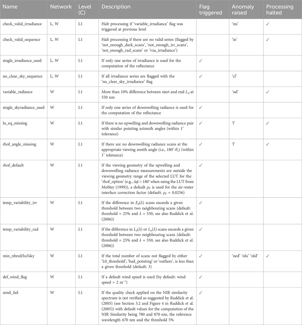
Table 4. Hypernets_processor flags applied during L1C processing.

3.3.1 L0A: Read raw data

While reading in the data, there are quality checks that verify whether the metadata.txt file is appropriate and all required raw data files exist. If these checks fail, an anomaly is raised (see Section 4.3) and the processing halts. There is also a quality check which checks whether the file with meteorological information exists. If it does not, an anomaly is added to the SQL database, but the processing is continued. In addition, for traceability, if the latitude and/or longitude are unknown (i.e., not included in the metadata.txt file), latitude and longitude are taken from the processor configuration file and the ‘lon_default’ and/or ‘lat_default’ flags are triggered. Next, the pointing accuracy of the pan/tilt is also verified. If the requested pan or tilt angle differs by more than 3° with the effective pan or tilt angle, the ‘bad_pointing’ flag is raised for the given scan.

3.3.2 L1A: Check raw data prior to calibrating

Before calibrating each of the individual scans in the L0 data, a number of quality checks is applied. If the spectrally integrated signal of a scan is more than 3 times the standard deviation, or more than 25% (whichever is largest) removed from the mean, it is masked and will not be used when averaging the series. This process is repeated until convergence and applied to the measured (ir)radiances and to the darks. The L0 data are also checked for saturation (digital number DN ≥ 64,000) and for discontinuities (missing values or ΔDN > 10⁴). A flag is also added to the L1 data if any of the dark scans have been masked by the above processes. Scans not satisfying the quality checks are flagged, but no data are removed at this stage.

3.3.3 L0B: Average valid scans

When averaging, only scans that passed the L1A quality checks are used. There are a few quality checks that check the number of scans being averaged is sufficient. By default, the threshold number of scans is three. If there are fewer than three scans for one of the dark, radiance or irradiance series, no reliable uncertainty can be calculated, and the series is flagged. If less than half of the radiance or irradiance scans of a series pass the L1A checks, the series is flagged, as this likely indicates something has gone wrong.

3.3.4 L1B: Check calibrated data are fit for purpose

After calibrating the L0B file, we check all the required measurements to form a standard sequence are included and have not been flagged by the previous ‘not_enough_dark_scans’, ‘not_enough_rad_scans’ or ‘not_enough_irr_scans’ flags. If any series are missing or flagged, the ‘series_missing’ is added to all the series in the sequence. If there are no valid radiance or irradiance measurements, the processing is halted.

Next, quality checks on the irradiance measurements are applied. First, their viewing angles are checked (which must be 180°, with a tolerance of 2°, as irradiance measurements have to be pointing up). Next, the irradiance is compared to a simulated clear-sky model. This clear sky model is made using the libRadtran radiative transfer software package (Emde et al., 2016), assuming its mid-latitude summer standard atmosphere and its standard desert surface (for land sites) and its standard ocean surface (for water sites). Note that the surface does not make a big difference as it is only second-order effects that affect the downwelling irradiance used in the clear sky model. The surface is assumed to be at sea-level and the TSIS solar irradiance model is used (Coddington et al., 2021). Given the downwelling irradiance measures the full hemisphere, the only relevant angle is the solar zenith angle. A clear sky model is calculated using solar zenith angles of 0°, 10°, 20°, 40°, 60°, 70° and 80°. These irradiance data are provided at 0.1 nm resolution to the hypernets_processor.

When performing the clear sky quality check, the irradiance data are band integrated to the HYPSTAR^® bands (which vary slightly from instrument to instrument), as defined by the calibration data, using the matheo⁸ tool. The measured HYPERNETS irradiances are then scaled (assuming cosine response) to match the nearest solar zenith angle among the provided clear sky models. In Figure 11, we show an example of the clear sky checks applied to the irradiance. We note that the clear sky models are not always very close, as a mid-latitude summer atmosphere at sea-level was used as opposed to a more realistic site-specific model. Therefore this quality check only fails if there are significant differences of more than 50% with the clear sky model (for more than 10% of the wavelength bands). Overcast conditions consistently trigger this quality flag.

Figure 11

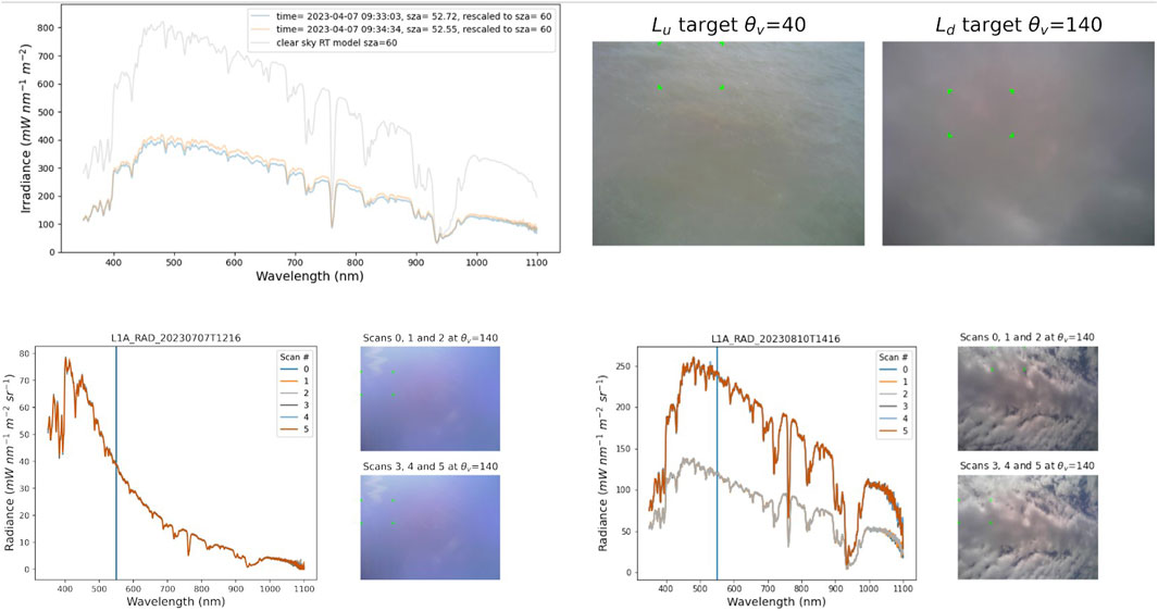
Figure 11. Example of the quality checks on the illumination applied in the L1B and L1C data processing for the downwelling irradiance and radiance, respectively. The top row shows the irradiance measurements not passing the ‘no_clear_sky_irradiance’ check taken at Zeebrugge MOW-1 Belgium (M1BE) site on the 2023–04–07 at 09:32 together with the simulated clear sky (for the same illumination geometries). Images of the sky (θ_v = 140°) and the water (θ_v = 40°) for this sequence are also shown. Bottom row shows (1) an example of downwelling radiance scans passing the quality criteria for constant downwelling radiance taken at WRUK on 2023–07–07 and the images taken with the camera during the measurements (bottom left panels), and, (2) an example of downwelling radiance scans not passing this quality check (variable_radiance flag is raised), and, the images taken with the camera during the measurements taken on 2023–08–10 at WRUK (bottom right panels).

Then, there is a quality check verifying that the irradiance has not changed more than 10% (after correcting for differences in solar zenith angle) between the measurements at the start and end of the sequence. At this stage the resulting irradiance series are flagged and the L1B file is produced. However if this ‘variable_irradiance’ check is triggered the processing will be halted at the L1C stage.

There are also some quality checks on the uncertainties. These check that there are no negative uncertainties and that less than 50% of the random uncertainties (i.e., less than half of the spectral channels) on radiance and irradiance have values below 100% (this indicates corrupted or dark data, e.g., measurements at night fail this check).

For the LANDHYPERNET network, there is an additional check that there is no strong discontinuity (larger than 25%) between the VNIR and SWIR parts of the spectrum for both radiances and irradiances.

3.3.5 L1C: Check if all required data for L1C processing is valid

Before interpolating the irradiances, there are a number of checks verifying the data are valid. If the ‘variable_irradiance’ flag was raised in previous levels, we cannot perform reliable interpolation and the processing is halted. Next, the processing is halted if there are no valid series for either radiance or irradiance (checking ‘not_enough_dark_scans’, ‘not_enough_irr_scans’, ‘not_enough_rad_scans’ or ‘vza_irradiance’ flags). When all irradiance series have the ‘no_clear_sky_irradiance’ flag, the processing is continued, as overcast products might still be useful to some users (available by request). A flag is added to all series to indicate this is a sequence without clear sky irradiance. No L1D/L2B data will be produced (and thus this data will not be provided publicly). When only one irradiance series is available (due to ‘vza_irradiance’ or missing measurements), the processing is continued, and the same irradiance is used for every radiance series (instead of temporally interpolating), with a correction for the changing solar zenith angle throughout the sequence. A flag is added to the entire sequence to indicate only one irradiance has been used.

For the WATERHYPERNET network, there are a number of additional quality checks. First, similarly to the ‘variable_irradiance’ flag, it checks if the downwelling sky radiance, L_d, at 550 nm remains constant over the entire sequence (i.e., coefficient of variation for L_d (550) < 10%). Indeed, if L_d varies significantly between the start and the end of the sequence, the downwelling sky radiance can not be temporally interpolated to the timestamps of the L_u scans and the processing is therefore halted. Note however that the threshold of 10% difference may be subject to further research in order to select the best threshold. Next, an anomaly (i.e., ‘l’) is raised and the processor is halted if the upwelling and downwelling radiance pair does not have a similar pointing azimuth angle (within 1° accuracy), or, if the viewing geometry does not satisfy θ_v for L_d equals 180-θ_v for L_u (within 1° accuracy).

The processor also checks for the temporal variability within each series. Scans for E_d, L_u and L_d at 550 nm, should not vary by more than a certain threshold with their neighbouring scans (default threshold is 25%). Note, those flags are not expected to be raised as scans with high temporal variability should have been removed by previous flags, i.e., ‘outliers’ or ‘L0_discontinuty’ flags. However, these flags are kept to ensure consistency with other common water network processing (Ruddick et al., 2006; Vansteenwegen et al., 2019).

The number of scans per series is important to assess the uncertainties. Hence, if the number of scans, not flagged by ‘bad pointing’, ‘outliers’, ‘L0_thresholds’, or ‘L0_discontinuity’, for E_d, L_u and L_d is below a given threshold, an anomaly is raised, and the processing is halted. The current default value is three which is a compromise between sequence duration and measurement replicates.

If the viewing geometry of the upwelling and downwelling radiance measurements are outside the viewing geometry range of the selected LUT for the ‘rhof_option’, the flag ‘rhof_default’ is raised. Similarly, a ‘def_wind_flag’ is used to trace spectra processed with a default wind speed value.

Finally, the flag ‘simil_fail’ is raised if the quality check applied on the NIR similarity spectrum is not verified as suggested by Ruddick et al. (2005). Note, this flag should only be considered for water types satisfying the NIR Similarity spectrum theory (i.e., clear to moderately turbid waters).

3.3.6 L2A: Calculate reflectance

Currently, no further quality checks are applied. For the WATERHYPERNET network, water radiance and reflectance are averaged only for the L_u scans which are not flagged for temporal variability, i.e., ‘temp_variability_irr’ and ‘temp_variability_rad’, or ‘rhof_default’.

3.3.7 Site-specific quality checks

The site-specific quality checks range from angular masks, i.e., viewing geometries that are expected to be affected by shadows or part of the installation (such as a mast) in the field-of-view, to quality checks that are very specific to the surface for a given site (e.g., ensuring vegetation is measured for the Wytham Woods UK (WWUK) site, or checking abnormal high reflectance values over clear or low turbid waters). Such site-specific checks often use thresholds (determined from analysis of the first months/year of data) checking the reflectance (or ratios of reflectances, e.g., epsilon for water sites, or NDVI for vegetated sites) at specific wavelengths. Additionally, the site owners can provide specific date-time ranges to mask, e.g., because something went slightly wrong during the deployment of the instrument (e.g., alignment).

Another important quality check is that the surface reflectances are compared to a time-series of similar measurements (matching viewing geometry and time of day) at the same site, to identify outliers so that they can be investigated. If these outliers are found to come from invalid data, further quality checks can be added to remove such cases.

The resulting site-specific masks are applied on a sequence-by-sequence basis to both L2A data (resulting in L2B dataset) and to the L1B dataset (resulting in L1D dataset). The same mask is applied to both L2A and L1B so that they remain consistent with each-other.

3.4 Uncertainties

3.4.1 Uncertainty propagation

The hypernets_processor uses a Monte Carlo (MC) approach (see Supplement one to the “Guide to the expression of uncertainty in measurement” (JCGM 101:2008, 2008), to propagate uncertainties and error-correlations between product levels. This MC approach is implemented using the punpy module from the open-source CoMet toolkit. punpy is a Python software package to propagate random, structured and systematic uncertainties through a given measurement function. For further info on punpy, we refer to De Vis & Hunt (in this issue), the CoMet website⁹ and the punpy documentation¹⁰.

In short, we first implement each of the processing steps as a numerical measurement function (e.g., measurement function in Section 3.2.2), i.e., a Python function which takes the input quantities (for which we are propagating the uncertainties) as arguments and returns the measurand (for which we are calculating the uncertainties as output). punpy then generates MC samples of the input quantities (taking into account the error correlation) proportional to the joint Probability Distribution Function (PDF) of the provided input quantities. Each of these samples is then run through the numerical measurement function to produce a sample of measurands. Finally, these output samples are analysed to obtain the uncertainties and error-correlation in the measurand. The uncertainties are propagated in this way through the measurement functions of each processing step discussed in Section 3.2.

3.4.2 Storing uncertainty information as digital effects tables

As previously mentioned, detailed error-correlation information is calculated as part of the uncertainty propagation. Storing this information in a space-efficient way is not trivial. To do this we use the obsarray module¹¹ of the CoMet toolkit. obsarray uses a concept called ‘digital effects tables’ to store the error-correlation information. This concept takes the parameterised error-correlation forms defined in the Quality Assurance Framework for Earth Observation (QA4EO) project¹² and stores them in a standardised metadata format. By using these parameterised error-correlation forms, it is not necessary to explicitely store the error-correlation along all dimensions. Instead only the error-correlation with wavelength is explicitly stored, and error-correlation with scans/series is captured as the ‘random’ or ‘systematic’ error-correlation forms.

Another benefit to using obsarray, is that it allows for straightforward encoding of the uncertainty and error-correlation variables. The error-correlation (with respect to wavelength) does not need to be known at a very high precision. It can be saved as an 8-bit integer (leading to about a 0.01 precision in the error-correlation coefficient). Similarly, the uncertainties can be encoded using a 16-bit integer to a precision of 0.01%. Together, these encodings significantly reduce the amount of space required to store the uncertainty information.

Finally, having the HYPERNETS products saved as ‘digital effects tables’ means they can easily be used in further uncertainty propagation where all the error-correlation information is automatically taken into account. See De Vis & Hunt (in this issue) and the CoMet toolkit examples¹³ for further information (note there is one example specific to HYPERNETS).

3.4.3 Uncertainty contributions

Three uncertainty contributions are tracked throughout the processing.

• Random uncertainty: Uncertainty component arising from the noise in the measurements, which does not have any error-correlation between different wavelengths or different repeated measurements (scans/series/sequences). The random uncertainties on the L0 data are taken to be the standard deviation between the scans that passed the quality checks. These uncertainties are then propagated all the way up to L2A.

• Systematic independent uncertainty: Uncertainty component combining a range of different uncertainty contributions in the calibration. Only the components for which the errors are not correlated between radiance and irradiance are included. These include contributions from the uncertainties on the distance, alignment, non-linearity, wavelength, lamp (power, alignment, interpolation) and panel (calibration, alignment, interpolation, back reflectance) used during the calibration. Since the same lab calibration is used within the hypernets_processor for repeated measurements (scans/series/sequences), the errors in the systematic independent uncertainty are assumed to be fully systematic (error-correlation of one) with respect to different scans/series/sequences. With respect to wavelength, we combine the different error-correlations of the different contributions and calculate a custom error-correlation matrix between the different wavelengths. These uncertainties are included in the L1A-L2A data products.

• Systematic uncertainty correlated between radiance and irradiance: Uncertainty component combining a range of different uncertainty contributions in the calibration. Only the components for which the errors are correlated between radiance and irradiance are included. This error-correlation means this component will become negligible when taking the ratio of radiance and irradiance (i.e., in the L2A reflectance products), which is why we separate it from the systematic independent uncertainty. The systematic uncertainty correlated between radiance and irradiance includes contributions from the uncertainties on the lamp (calibration, age) because the same lamp was used for the radiance and irradiance HYPSTAR calibrations in Tõravere. Since the same lab calibration is used within the hypernets_processor for repeated measurements (scans/series/sequences), the errors in the systematic independent uncertainty are assumed to be fully systematic (error-correlation made up of ones) with respect to different scans/series/sequences. With respect to wavelength, we combine the different error-correlations of the different contributions and calculate a custom error-correlation matrix between the different wavelengths. These uncertainties are present in the L1A-L1C products.

The temperature and spectral straylight uncertainties will be improved in future versions (Section 6). Additionally, there is an uncertainty to be added on the HYPSTAR responsivity change since calibration (drift/ageing of spectrometer and optics). More post-deployment calibrations are necessary before we can quantify this contribution. Other uncertainty contributions not yet included in the uncertainty budget will also be considered in the future, such as uncertainties on the sensitivity to polarisation, uncertainties in the cosine response of the irradiance optics, the effects of the platform/mast on the observed upwelling radiances (e.g., Talone and Zibordi, 2018), or on the air-water interface reflectance corrections. Uncertainties on the Spectral Response Functions (SRF) of the radiance and irradiance sensors (particularly the difference between the two is important when calculating reflectance) should also be considered (see also Ruddick et al., 2023). To account for these missing uncertainty contributions, a placeholder uncertainty of 2% is added to the systematic independent uncertainty, assuming systematic spectral correlation. In the strong atmospheric absorption features (i.e., 757.5–767.5 nm and 1,350–1,390 nm), an additional placeholder uncertainty of 50% (assuming random spectral error correlation) is added to account for the difference in SRF becoming dominant. Examples of the different uncertainty contributions are shown in Section 5.3.

4 HYPERNETS products

4.1 Product format, variables and metadata

The main output files produced by the hypernets_processor are in NetCDF CF-convention version 1.8 format. There are also plots, typically produced in png format, and SQL databases (see Section 4.3).

The different NetCDF files contain a range of different variables and metadata. The main measurands, as well as their dimensions for the different levels of data files are described in Table 2. For these measurand variables, there are also uncertainty variables for each of the components described in Section 3.4, as well as error-correlation variables for the systematic uncertainty components.

In addition to these there are coordinate variables, wavelength and series/scans, as well as a number of common variables (i.e., present in each of the data products) that provide additional details about the measurement. Acquisition time, viewing zenith and azimuth angle, solar zenith and azimuth angle are examples of common variables with series or scans as dimension. Bandwidth is also a common variable which has the wavelength dimension. Then there are a few additional variables such as the quality flag variable and variables specifying the number of valid and total VNIR scans and specifying the number of valid and total SWIR scans (for the LANDHYPERNET network).

There are also a number of variables that are only present in some of the data products. For example, there is some additional information in the L0A files, such as integration times, values of the accelerometers, the requested and returned pan/tilt angles. This information is propagated to the L1A and L0B files, but not beyond.

The quality flag field consists of 32 bits. Every bit is related to the absence or presence of a flag as described in Section 3.3. The quality flag value given in each data level is the compound value of the specific bits of each raised flag. The specific flags associated with each bit are given in the quality flag field metadata. Some flags are left as placeholders for future updates. Tables 3, 4 present the flags used in the current version.

The are is also a range of metadata contained within the files. For each variable, there is metadata such as the standard name, long name, units and uncertainty components (where relevant). The uncertainty variables will have additional metadata describing their error correlation (see Section 3.4). Finally, there is also a range of global metadata, describing information about how, and when the data was processed, what data files it used, information about the site (e.g., latitude and longitude) etc.

4.2 File naming

The naming convention is intended to allow the unique identification of all product files and to summarise the contents. It is composed of a defined sequence of data fields, separated by an underscore. For the HYPERNETS measurement data, the file name is composed as follows:

SYSTEM NETWORK SITEID LEVEL TYPE ACQUISITIONDATETIME PROCESSINGDATETIME_version.nc.

where.

• System: “HYPERNETS”

• Network: Name of product network, i.e., W and L for WATERHYPERNET and LANDHYPERNET network, respectively.

• Siteid: Abbreviated site names defined in Table 5.

• Level: Data processing Level as defined in Table 2. For the RGB images the level is “IMG”.

• Type: Name of product type. Values may be abbreviated product type names defined in Table 2.

• Acquisitiondatetime: Denotes the acquisition datetime (start of sequence) as UTC, formatted as “YYYYMMDDTHHMM”.

• Processingdatetime: Denotes the processing datetime as UTC, formatted as “YYYYMMDDTHHMM”.

• Zenith: For the RGB images only–viewing nadir angle ranging from 0° (looking down) to 180° (looking up).

• Azimuth: For the RGB images only and the L1C and L2A/B WATERHYPERNET network files–relative azimuth angle between Sun and sensor ranging from 0° to 360°.

• Version: Denotes data version number, formatted as “vX.X” as described in Section 2.5.

For instance, for a L1B product processed by the hypernets_processor version two of WATERHYPERNET network acquired at Blankaart South at 11:30 UTC on 2023–10–04 and processed at 11:30 UTC on 2023–10–05, the filename should be:

HYPERNETS_W_BSBE_L1B_RAD_20231004T1130_20231005T1130_v2.0.nc,

and the related L2A files for standard measurement protocols taken at 90° and 135° Δϕ should be:

HYPERNETS_W_BSBE_L1B_RAD_20231004T1130_20231005T1130_v2.0.nc, and,

HYPERNETS_W_BSBE_L2A_REF_20231004T1130_20231005T1130_135_v2.0.nc.

Table 5 defines the abbreviated name convention applicable to the individual HYPERNETS sites. Site name convention is a 4 letter abbreviation [LLCC] with LL standing for the location and CC for the country.

Table 5

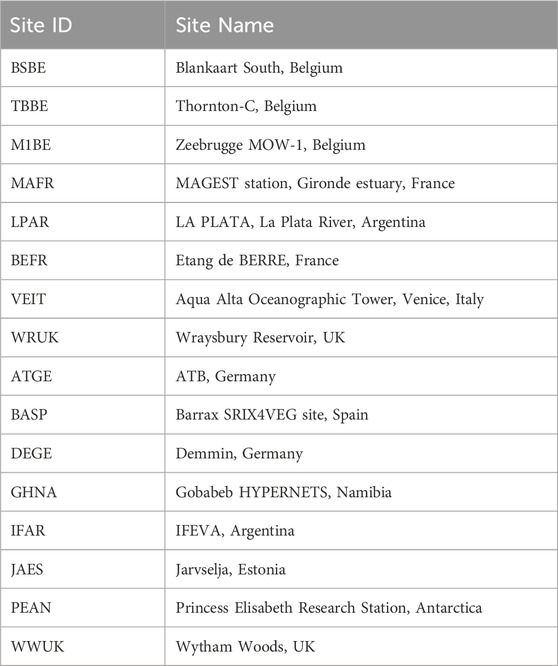
Table 5. Examples of site name conventions for water and land sites.

4.3 SQL databases

The hypernets_processor produces SQL Database entries to keep track of successfully processed sequences and anomalies in the processing. These entries are combined into the following three databases, each stored in the SQLite format:¹⁴

• Archive Database: SQLite database listing all successfully processed data products, together with auxiliary information to enable queries (e.g., product_name, datetime, sequence_name, site_id, latitude, longitude, solar and viewing angles, etc.).

• Anomaly Database: There are a number of anomalies to track where there are issues in the processing of the data (e.g., incomplete sequence data, instrument failure etc.). The different anomalies are defined above in Tables 3, 4 as well as in the hypernets_processor documentation. Each of the anomalies is identified with a letter and every occurrence is stored in the Anomaly SQLite database, together with auxiliary information to enable queries (e.g., sequence_name, site_id, datetime, viewing and solar angles, etc.). Some of these anomalies will raise an error (e.g., metadata file missing), and cause the processing of the data to be stopped. Other anomalies (e.g., clear sky check failed) indicate an issue, but do not halt the processing of the data (e.g., measurements with overcast conditions might still be useful to some users). In such cases, a quality flag is always added to the data so that users can easily identify the affected sequences without having to look in the anomaly database (see Section 3.3).

• Metadata Database: SQLite database of all network metadata, e.g., site info, instrument info etc. Contains all the metadata that is also present in the product files (stored in database to enable querying this information).

These databases can be used to produce processing statistics, or to find a set of sequences/anomalies that matched a certain set of criteria using SQL queries.

4.4 Data management and distribution

To follow the Findable-Accessible-Interoperable and Reusable principles (FAIR), particular attention is given to the data format and metadata, and, data accessibility. Files are in the NetCDF CF-convention version 1.8 format. Common metadata (e.g., metadata section added with each data product) follow the INSPIRE directives¹⁵ in accordance with the EN ISO 19115 for the metadata elements and the Dublin Core Metadata Initiative¹⁶. Instrument, component and system metadata are bound by a unique metadata key (i.e., system_id) allowing to trace the history of the system (e.g., replacement, maintenance, system updates or instrument setup improvements).

The distribution of Near Real-Time (NRT, 24 h between data acquisition and data availability) LANDHYPERNET and WATERHYPERNET data will happen through the data portals for the LANDHYPERNET (www.landhypernet.org.uk) and WATERHYPERNET (www.waterhypernet.org). However, during the current prototype phase, where improvement of the quality checks is still ongoing, and further site-specific quality checks are still being added by the site-owners, these data portals are restricted to consortium members. In addition, for the WATERHYPERNET network the distribution may be delayed to ensure that the NCEP/GDAS forecast data for wind speed are made available for the latest sequence (should be less than 24 h). Data transfer from the system to the server may also delay the NRT processing (e.g., due to poor 4G connections on the field). In the near future, these data portals will be opened to the public and will become the reference source of data for HYPERNETS.

In the meantime, a subset of the HYPERNETS data until 2023–04–31 is publicly available and can be found on Zenodo (Brando et al., 2023; Brando and Vilas, 2023; De Vis et al., 2023; Dogliotti et al., 2023; Doxaran and Corizzi, 2023a; Doxaran and Corizzi, 2023b; Piegari et al., 2023; Goyens and Gammaru, 2023; Morris et al., 2023; Saberioon et al., 2023a; Saberioon et al., 2023b; Sinclair et al., 2023). The initial datasets provided here in June 2023 were produced using the v1.0 of the hypernets_processor (see Section 2.5). A new version of the datasets on Zenodo will be released upon publication of this paper, using the v2.0 of the hypernets_processor.

5 Results

5.1 LANDHYPERNET network example

In this section, we discuss the results of the processing of a few example land sequences. Two examples are included, one for the WWUK site on 2022–06–26 at 11:40 UTC and one for the GHNA site on 2022–08–04 at 10:00 UTC. Figure 12 shows a few of the plots created by the hypernets_processor for these two sequences.

Figure 12

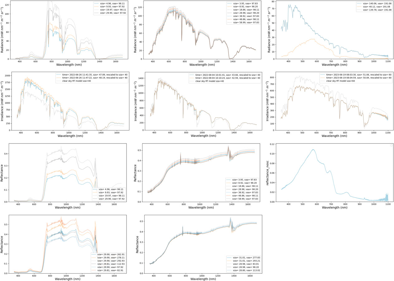
Figure 12. hypernets_processor plots for the WWUK site on the 2022–06–26 at 11:40 (left column), GHNA site on the 2022–08–04 at 10:00 (centre column) and the water site M1BE on 2022–06–19 at 08:02 (right column). The top row shows the L1B radiances at different viewing zenith angles, second row L1B irradiances together with clear sky model used in quality check. The third row shows the L2A reflectances at different viewing zenith angles for land and the non similarity corrected reflectance for water. The bottom row shows the L2A reflectances at different azimuth angles for land. Note the different wavelength range along the x-axis for the land (WWUK and GHNA) and water (M1BE) sites.

The radiance plots show a lot more variability between different viewing zenith angles for the WWUK site than for the GHNA site, which is to be expected as GHNA is expected to be especially homogeneous and near-Lambertian, whereas the WWUK is a vegetated site, which has spatial heterogeneity and significant bidirectional reflectance distribution function (BRDF) effects. When the irradiances are inspected and compared to the clear sky models, we see that for each of these cases, the clear-sky model matches the observed radiances quite well. We note that this will not always be the case, as the clear sky model does not take into account the different surface reflectance, pressure or aerosol properties for each site.

The bottom two rows of Figure 12 show how the surface reflectances vary with viewing zenith and azimuth angles. Typical reflectances for vegetation (WWUK) and deserts (GHNA) are found. Again, much more variation is seen between the reflectances for the different geometries for WWUK than for GHNA, as expected. There are some blips in the reflectance around the absorption features (e.g., around 760 nm and 1,370 nm), which are likely caused by differences in the SRF of the radiance and irradiance sensors (See also Ruddick et al., 2023). Uncertainties have been increased to account for these SRF differences (see Sections 3.4; 5.3).

5.2 WATERHYPERNET network example

The last column in Figure 12 shows the plots provided by the WATERHYPERNET processor for a sequence at M1BE on 2022–06–19 at 08:02 UTC. Measurements were made at a relative azimuth angle, Δϕ, of 90° and the wind speed retrieved from NCEP/GDAS was around 6.2 m⁻¹. Top plot shows the averaged radiance scans for two series of L_d (two times three scans) and one series of L_u (six scans). It was a clear blue sky at M1BE on that day, and illumination during the sequence seemed to be constant. This is confirmed by the downwelling radiance (top right panel) and irradiance (second row right panel) series that are similar at the start and the end of the sequence. The bottom right panel show the final averaged reflectance product, i.e., the L2A reflectance. This figure shows that the water at M1BE was green and turbid on that day with a reflectance peak around 550 nm and relatively high red-NIR values.

5.3 Uncertainty example

We have illustrated the typical relative uncertainties of the LANDHYPERNET and WATERHYPERNET products in Figure 13, using the same three examples (GHNA, WWUK & M1BE) as discussed in the previous sections. For radiance (top row), the three uncertainty components are shown (one line for each series) for the three sites. The two systematic components are very similar between each of the sites, though for the water example (M1BE), the wavelength range is different compared to the land sites. This similar shape of the systematic uncertainties is expected as the instruments deployed at three sites are calibrated in the same way and thus have similar calibration uncertainties. These systematic components are also the same for each sequence for these sites, as the same calibration is applied for every sequence. The random uncertainty on the radiance is more variable, as it is dependent on illumination conditions, the nature of the target, and the stability of the instrument. Smaller relative uncertainties are found for brighter surfaces. Note the difference in wavelength range between the land and water sites with, subsequently, higher uncertainties in the blue and NIR spectral for the water site as it corresponds to the extremes of the wavelength range. The uncertainty plots for irradiance in Figure 13 are very similar than for radiance. The main difference, in particular for the land sites, is that there are fewer series (only two), and the relative random uncertainties are a bit smaller (due to higher signal in irradiance).

Figure 13

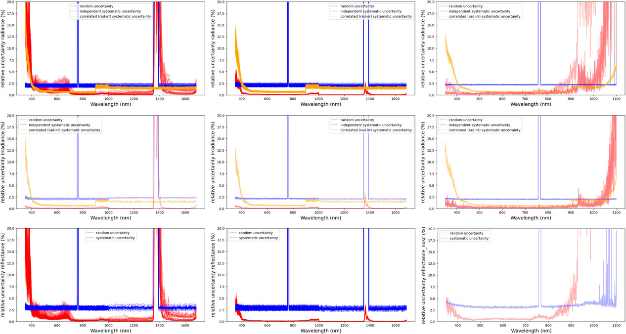
Figure 13. Example hypernets_processor plots illustrating the uncertainties (in percent) on L1B radiances (top row), L1B irradiances (second row) and L2A reflectances (third row) for the WWUK site on 2022–06–26 at 11:40 (left column), GHNA site on 2022–08–04 at 10:00 (centre column) and the water site M1BE on 2022–06–19 at 08:02 (right column). Note the different wavelength range along the x-axis for the land (WWUK and GHNA) and water (M1BE) sites.

For reflectance, there are only two uncertainty components as the systematic component for which the errors in radiance and irradiance are correlated become negligible. For most wavelengths, the (independent) systematic component dominates over the random uncertainties. The random uncertainties will become even smaller when averaging measurements or integrating over the SRF of a satellite sensor (e.g., De Vis et al., in this issue), as opposed to the systematic uncertainties which will remain constant. For the water site, the random uncertainty is higher compared to the systematic uncertainty in the NIR spectral range. This is due to the usually very low water signal in this spectral range.

Finally, Figure 14 top row shows the error-correlation between the different wavelength channels of the systematic component(s) for the L1B radiances of the GHNA example, i.e., the error-correlation matrix for the independent systematic uncertainty (left) and the correlated (between radiance and irradiance) systematic uncertainty (right). The bottom plots show the error-correlation for the L2A (independent) systematic uncertainties on reflectance for the land (left) and water (right) examples (GHNA and M1BE, respectively). For the independent systematic error correlations for land, there is a strong correlation between the wavelengths within the VNIR and SWIR sensors, but not between VNIR and SWIR. The strong wavelength correlation comes from various components, with a strong contribution from the placeholder uncertainty. As this placeholder is replaced by more realistic contributions, this error-correlation structure might become more complex. For the water example, correlations remain high at all wavelengths between the blue and red wavelengths.

Figure 14

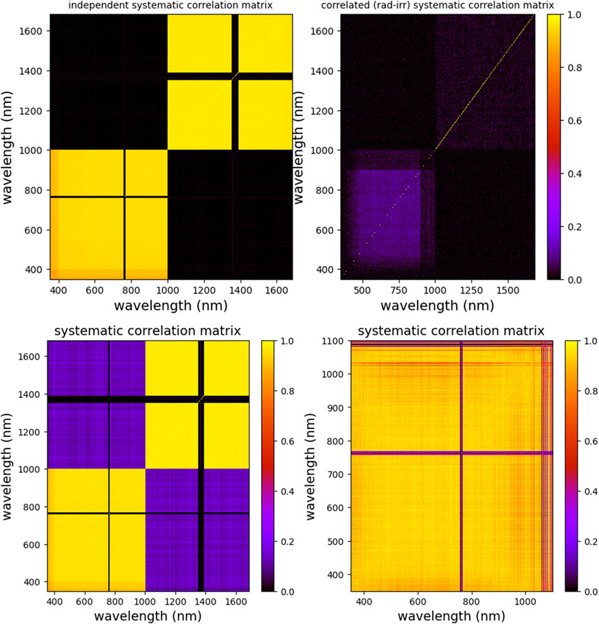
Figure 14. Example of the error-correlation matrices for the systematic independent uncertainty on GHNA L1B radiance (top left), the systematic uncertainty on GHNA L1B radiance correlated between radiance and irradiance (top right), the systematic uncertainty on GHNA L2A reflectance (bottom left) and systematic uncertainty on M1BE L2A reflectance (bottom right). Note that the M1BE error-correlation matrices have a reduced wavelength range.

5.4 Processing statistics of H2020 HYPERNETS data

In this section we briefly provide some of the processing statistics for both the LANDHYPERNET and WATERHYPERNET networks until the end of April 2023. for the LANDHYPERNET, there were a total of 12,190 sequences acquired. 11,802 of these (97%) were successfully processed to L2A. The remainder had an anomaly which halted the processing (Section 3.3). Stringent site specific quality checks were applied to the L2A data, and a total of 4,256 sequences were provided on the Zenodo database.

For the WATERHYPERNET, there were 55,514 sequences acquired. 44,412 of these (80%) were succesfully processed to L2A. Stringent site specific quality checks were applied to the L2A data, and a total of 4,931 sequences were provided on the Zenodo database. Note that the data provided on Zenodo are still a subset of the entire dataset and that the number of processed and quality checked sequences is expected to increase since the first version of the processor has been considerably improved (e.g., additional and more appropriate flagging, processing issues and bugs have been solved, accounting for different relative azimuth angles, retrieving wind speed from a different data source, i.e., NCEP/GDAS) to the current v2.0 of the hypernets_processor.¹⁷

6 Future work

There are a number of improvements that are foreseen in the near future.

• There are a number of improvements that will be made to the calibration measurement function, such as the inclusion of a temperature and spectral straylight correction. As soon as lab-based characterisation of these effects is concluded, appropriate corrections will be implemented and added to the calibration measurement function (see Section 3.3.2).

• Post-deployment calibration will be implemented in the future. This means it would be possible to do a reprocessing of the data between the calibration dates and interpolate the calibration data between the pre-deployment data and post-deployment data. Post-deployment data should be gathered prior to any cleaning being done to the instrument. Further investigations will be performed to compare results from interpolating calibrations, to calibrations done using the previous available date. This will also include assessments of the uncertainty on the calibration due to drift/ageing of the sensor and optics.

• There are still missing uncertainty contributions that currently are just provided as a combined placeholder uncertainty (see Section 3.4). These include uncertainties related to the temperature and spectral straylight corrections, as well as uncertainties due to the angular accuracy, polarisation, the effects of the platform/mast on the observed upwelling radiances (e.g., Talone and Zibordi, 2018) and the uncertainty in the retrieval of the air-water interface correction methodology. Uncertainties on the SRF will also be more precisely included. All these uncertainties need dedicated studies in order to be quantified, and will be added to the hypernets_processor as soon as they have been quantified. The placeholder uncertainty will be adjusted when new uncertainty components are added, with the aim of eventually not needing any placeholder uncertainty any more.

• The current angular tolerance on the viewing zenith angle for the irradiance measurements is set to 2°. This leads to acceptable irradiances, but improvements can still be made by correcting the irradiance measurements for any deviation from vza = 180, taking into account the solar azimuth angles, and relative azimuth angles.

• Further investigations will be performed of the potential improvements of using high resolution models in the spectral and temporal interpolation of the irradiances (See Section 3.2.4.1).

• In future versions of the processor we will further investigate whether using a sliding average would be useful where, for the overlapping wavelengths, a weighted (by inverse of uncertainties) mean is taken between VNIR and SWIR so that there is a smooth transition. The overlapping wavelength range spans from about 880–1,100 nm, with worse performance towards the ends of the wavelength range of each detector.

• Work is ongoing to continuously improve the common quality checks being applied as part of the automated processing, as well as the site-specific quality checks. These improvements will include improved checks such as angular masks for shadowing effects by the mast/platform, non-linearity checks and more robust comparisons with expected reflectance.

• BRDF modelling will be investigated for a number of LANDHYPERNET sites. This would allow for better outlier detection compared to the BRDF model, as well as allow interpolation over missing geometries.

• The current standard protocol for measurement of water reflectance uses external sources for the retrieval of the wind speed and approximates the air–water interface reflectance factor following Mobley (1999). However, it is known that these methods present some limitations (see Goyens and Ruddick (2023) and references therein). In the future, new methods and models may be explored and integrated into the processor.

• The LANDHYPERNET and WATERHYPERNET data portals (see also Section 4.4) will be fully opened to the public.

• A web interface allowing to visualise the latest incoming data, the archived data, and the anomalies and flags of the processed data, may also be build to help debugging and tracing issues in the sensor deployments and the processing.

• An API will be developed to access and download the L1D and L2B HYPERNETS data through a Python tool which will also include command-line functionality. This API will use credentials for the LANDHYPERNET and WATERHYPERNET data portals.

• Future version of the processor might make additional data products available to the public, such as irradiance and surface reflectance measurements during fully overcast conditions (which are not useful for satellite validation but might be of interest to other user communities), and products including additional water (e.g., turbidity) and atmospheric (e.g., aerosol optical depth) products. Any of these additional products would require significant validation before they could be made public so are not expected in the near future.

Some of these improvements will be present in the next major version (v3.0) of the hypernets_processor.¹⁸ The documentation¹⁹ will also be kept up to date with any modifications made to the hypernets_processor.

7 Conclusion

The hypernets_processor is a software package for ground processing of the hyperspectral HYPSTAR^® data from the autonomous field sites of the LANDHYPERNET and WATERHYPERNET networks. it continuously processes new acquisitions taken by the HYPSTAR^® instrument, through various processing levels, to the surface reflectance products required for validation of satellite measurements. Uniquely for this type of processing, multiple different types of uncertainty (including error-correlations) are propagated through each of the processing levels. The processor is now operationally running for a series of networked validation sites, revealing plausible results and a well constrained uncertainty budget.

Data availability statement

The datasets generated for this study (Brando et al., 2023; Brando and Vilas, 2023; De Vis et al., 2023; Dogliotti et al., 2023; Doxaran and Corizzi, 2023a; Doxaran and Corizzi, 2023b; Piegari et al., 2023; Goyens and Gammaru, 2023; Morris et al., 2023; Saberioon et al., 2023a; Saberioon et al., 2023b; Sinclair et al., 2023) can be found on Zenodo (https://zenodo.org/).

Author contributions

PD: Conceptualization, Data curation, Investigation, Methodology, Software, Validation, Visualization, Writing–original draft. CG: Conceptualization, Data curation, Investigation, Methodology, Software, Validation, Visualization, Writing–original draft. SH: Conceptualization, Methodology, Software, Writing–review and editing. QV: Methodology, Writing–review and editing. KR: Funding acquisition, Project administration, Writing–review and editing. AB: Funding acquisition, Project administration, Writing–review and editing.

Funding

The author(s) declare that financial support was received for the research, authorship, and/or publication of this article. The HYPERNETS project is funded by the European Union’s Horizon 2020 research and innovation program under grant agreement No. 775983 and by the HYPERNET-POP project funded by the European Space Agency (contract No. 4000139081/22/I-EF). This work (and the CoMet toolkit used within) has also received funding from the ESA-funded Instrument Data quality Evaluation and Assessment Service-Quality Assurance for Earth Observation (IDEAS-QA4EO) contract funded by ESA-ESRIN (No. 4000128960/19/I-NS) and the UK’s Department for Science, Innovation and Technology (DSIT) National Measurement System (NMS) programme.

Acknowledgments

The HYPERNETS partners, especially Tartu University and Sorbonne University are thanked for technical support and development of the HYPSTAR^® instrument and system. The HYPERNETS PI (Kevin Ruddick), co-PIs (Agnieszka Bialek, Vittorio Brando, Ana Dogliotti, David Doxaran, Joel Kuusk, Mohammadmehdi Saberioon) as well as all other contributors are gratefully acknowledged for their useful inputs, discussion and comments. Paul Green and Joel Kuusk are thanked for useful comments.

Conflict of interest

The authors declare that the research was conducted in the absence of any commercial or financial relationships that could be construed as a potential conflict of interest.

Publisher’s note

All claims expressed in this article are solely those of the authors and do not necessarily represent those of their affiliated organizations, or those of the publisher, the editors and the reviewers. Any product that may be evaluated in this article, or claim that may be made by its manufacturer, is not guaranteed or endorsed by the publisher.

Footnotes

¹https://kosmos.ut.ee/en/laboratory

²https://github.com/HYPERNETS/hypernets_processor

³https://hypernets-processor.readthedocs.io/en/latest/content/developers/getting_started.html

⁴https://hypernets-processor.readthedocs.io/en/latest/content/users/adhoc.html

⁵https://hypernets-processor.readthedocs.io/en/latest/content/users/automated.html

⁶https://kosmos.ut.ee/en/laboratory

⁷https://comet-maths.readthedocs.io/en/latest/content/interpolation_atbd.html

⁸https://matheo.readthedocs.io/en/latest/

⁹www.comet-toolkit.org

¹⁰https://punpy.readthedocs.io/en/latest/

¹¹https://obsarray.readthedocs.io/en/latest/

¹²www.QA4EO.org

¹³https://www.comet-toolkit.org/examples/

¹⁴https://hypernets-processor.readthedocs.io/en/latest/content/atbd/products/anomalies.html

¹⁵http://inspire.ec.europa.eu/glossary/Metadata

¹⁶https://www.dublincore.org/specifications/dublin-core/dcmi-terms/

¹⁷https://landhypernet.org.uk/

¹⁸https://waterhypernet.org/

¹⁹https://hypernets-processor.readthedocs.io/en/latest/

References

Alonso, K., Bachmann, M., Burch, K., Carmona, E., Cerra, D., de los Reyes, R., et al. (2019). Data products, quality and validation of the dlr earth sensing imaging spectrometer (desis). Sensors 19, 4471. doi:10.3390/s19204471

PubMed Abstract | CrossRef Full Text | Google Scholar

Bouvet, M., Thome, K., Berthelot, B., Bialek, A., Czapla-Myers, J., Fox, N. P., et al. (2019). Radcalnet: a radiometric calibration network for earth observing imagers operating in the visible to shortwave infrared spectral range. Remote Sens. 11, 2401. doi:10.3390/rs11202401

CrossRef Full Text | Google Scholar

Brando, V., Gonzalez Vilas, L., Bresciani, M., Mangano, S., Concha, J. A., and Goyens, C. (2023). Initial sample of HYPERNETS hyperspectral water reflectance measurements for satellite validation at lake garda, GAIT site (Italy). Zendo. doi:10.5281/zenodo.8057823

CrossRef Full Text | Google Scholar

Brando, V., and Vilas, L. G. (2023). Initial sample of HYPERNETS hyperspectral water reflectance measurements for satellite validation from the VEIT site (Italy). Zendo. doi:10.5281/zenodo.8057531

CrossRef Full Text | Google Scholar

Coddington, O. M., Richard, E. C., Harber, D., Pilewskie, P., Woods, T. N., Chance, K., et al. (2021). The tsis-1 hybrid solar reference spectrum. Geophys. Res. Lett. 48, e2020GL091709. doi:10.1029/2020GL091709

PubMed Abstract | CrossRef Full Text | Google Scholar

De Vis, P., Bialek, A., and Sinclair, M. (2023). Initial sample of HYPERNETS hyperspectral surface reflectance measurements for satellite validation from the Gobabeb site in Namibia. Zendo. doi:10.5281/zenodo.8039303

CrossRef Full Text | Google Scholar

Dogliotti, A. I., Piegari, E., Rubinstein, L., and Perna, P. (2023). Initial sample of HYPERNETS hyperspectral water reflectance measurements for satellite validation from the LPAR site (Argentina). Zendo. doi:10.5281/zenodo.8057728

CrossRef Full Text | Google Scholar

Doxaran, D., and Corizzi, A. (2023a). Initial sample of HYPERNETS hyperspectral water reflectance measurements for satellite validation at berre coastal lagoon, BEFR site (France). Zendo. doi:10.5281/zenodo.8057777

CrossRef Full Text | Google Scholar

Doxaran, D., and Corizzi, A. (2023b). Initial sample of HCYPERNETS hyperspectral water reflectance measurements for satellite validation at the mouth of the gironde estuary, MAFR site (France). Zendo. doi:10.5281/zenodo.8057789

CrossRef Full Text | Google Scholar

Emde, C., Buras-Schnell, R., Kylling, A., Mayer, B., Gasteiger, J., Hamann, U., et al. (2016). The libradtran software package for radiative transfer calculations (version 2.0.1). Geosci. Model Dev. 9, 1647–1672. doi:10.5194/gmd-9-1647-2016

CrossRef Full Text | Google Scholar

Goryl, P., Fox, N., Donlon, C., and Castracane, P. (2023). Fiducial reference measurements (frms): what are they? Remote Sens. 15, 5017. doi:10.3390/rs15205017

CrossRef Full Text | Google Scholar

Goyens, C., De Vis, P., and Hunt, S. E. (2021). “Automated generation of hyperspectral fiducial reference measurements of water and land surface reflectance for the hypernets networks,” in 2021 IEEE International Geoscience and Remote Sensing Symposium IGARSS, Brussels, Belgium, 11-16 July 2021 (IEEE), 7920–7923. doi:10.1109/IGARSS47720.2021.9553738

CrossRef Full Text | Google Scholar

Goyens, C., and Gammaru, A. (2023). Initial sample of HYPERNETS hyperspectral water reflectance measurements for satellite validation at the measurement tower MOW1, M1BE site (Belgium). Zendo. doi:10.5281/zenodo.8059881

CrossRef Full Text | Google Scholar

Goyens, C., and Ruddick, K. (2023). Improving the standard protocol for above-water reflectance measurements: 1. estimating effective wind speed from angular variation of sunglint. Appl. Opt. 62, 2442–2455. doi:10.1364/AO.481787

PubMed Abstract | CrossRef Full Text | Google Scholar

Ishizaka, J., Yang, M., Fujii, N., Katano, T., Hori, M., Mine, T., et al. (2022). Use of aeronet-oc for validation of sgli/gcom-c products in ariake sea, Japan. J. Oceanogr. 78, 291–309. doi:10.1007/s10872-022-00642-9

CrossRef Full Text | Google Scholar

JCGM 100:2008 (2008). Evaluation of measurement data — Guide to the expression of uncertainty in measurement. Joint Committee for Guides in Metrology. JCGM 100:2008.

Google Scholar

JCGM 101:2008 (2008). Evaluation of measurement data — Supplement 1 to the “Guide to the expression of uncertainty in measurement” — propagation of distributions using a Monte Carlo method. Joint Committee for Guides in Metrology. JCGM 101:2008.

Google Scholar

Mobley, C. D. (1999). Estimation of the remote-sensing reflectance from above-surface measurements. Appl. Opt. 38, 7442–7455. doi:10.1364/AO.38.007442

PubMed Abstract | CrossRef Full Text | Google Scholar

Mobley, C. D. (2015). Polarized reflectance and transmittance properties of windblown sea surfaces. Appl. Opt. 54, 4828–4849. doi:10.1364/AO.54.004828

PubMed Abstract | CrossRef Full Text | Google Scholar

Morris, H., Bialek, A., Sinclair, M., and De Vis, P. (2023). Initial sample of HYPERNETS hyperspectral surface reflectance measurements for satellite validation from the Wytham Woods site in the United Kingdom. Zendo. doi:10.5281/zenodo.7962557

CrossRef Full Text | Google Scholar

National Centers for Environmental Prediction, National Weather Service, NOAA, U.S. Department of Commerce (2015). Ncep gdas/fnl 0.25 degree global tropospheric analyses and forecast grids. NOAA.

Google Scholar

Niro, F., Goryl, P., Dransfeld, S., Boccia, V., Gascon, F., Adams, J., et al. (2021). European space agency (esa) calibration/validation strategy for optical land-imaging satellites and pathway towards interoperability. Remote Sens. 13, 3003. doi:10.3390/rs13153003

CrossRef Full Text | Google Scholar

Piegari, E., Dogliotti, A., Grings, F., Perna, P., Rubinstein, L., and Cordon, G. (2023). Initial sample of HYPERNETS hyperspectral surface reflectance measurements for satellite validation from the IFEVA site in Argentina. Zendo. doi:10.5281/zenodo.8048425

CrossRef Full Text | Google Scholar

Ruddick, K., De, V., Ab, C., and Mol, B. (2005). Use of the near infrared similarity reflectance spectrum for the quality control of remote sensing data. Proc. SPIE - Int. Soc. Opt. Eng. 5885, 615152. doi:10.1117/12.615152

CrossRef Full Text | Google Scholar

Ruddick, K. G., De Cauwer, V., Park, Y.-J., and Moore, G. (2006). Seaborne measurements of near infrared water-leaving reflectance: the similarity spectrum for turbid waters. Limnol. Oceanogr. 51, 1167–1179. doi:10.4319/lo.2006.51.2.1167

CrossRef Full Text | Google Scholar

Ruddick, K. G., De Vis, P., Goyens, C., Kuusk, J., Lavigne, H., and Vanhellemont, Q. (2023). “Second derivative water reflectance spectra for phytoplankton species detection: origin, impact, and removal of spectral wiggles,” in Remote sensing of the ocean, sea ice, coastal waters, and large water regions 2023. Editors C. R. B. Jr., and X. Neyt (International Society for Optics and Photonics SPIE). doi:10.1117/12.2684336

CrossRef Full Text | Google Scholar

Ruddick, K. G., Voss, K., Boss, E., Castagna, A., Frouin, R., Gilerson, A., et al. (2019). A review of protocols for fiducial reference measurements of water-leaving radiance for validation of satellite remote-sensing data over water. Remote Sens. 11, 2198. doi:10.3390/rs11192198

CrossRef Full Text | Google Scholar

Saberioon, M., Spengler, D., Hohmann, C., and Itzerott, S. (2023a). Initial sample of HYPERNETS hyperspectral surface reflectance measurements for satellite validation from the agricultural land at demmin, Germany. Zendo. doi:10.5281/zenodo.8048348

CrossRef Full Text | Google Scholar

Saberioon, M., Spengler, D., Hohmann, C., Wille, C., and Itzerott, S. (2023b). Initial sample of HYPERNETS hyperspectral surface reflectance measurements for satellite validation from the bare soil at marquardt, Germany. Zendo. doi:10.5281/zenodo.8044522

CrossRef Full Text | Google Scholar

Sinclair, M., Morris, H., Bialek, A., De Vis, P., Gammaru, A., and Goyens, C. (2023). Initial sample of HYPERNETS hyperspectral surface reflectance measurements for satellite validation from the barrax site in Spain. Zendo. doi:10.5281/zenodo.8060798

CrossRef Full Text | Google Scholar

Talone, M., and Zibordi, G. (2018). Non-linear response of a class of hyper-spectral radiometers. Metrologia 55, 747–758. doi:10.1088/1681-7575/aadd7f

CrossRef Full Text | Google Scholar

Vansteenwegen, D., Ruddick, K., Cattrijsse, A., Vanhellemont, Q., and Beck, M. (2019). The pan-and-tilt hyperspectral radiometer system (PANTHYR) for autonomous satellite validation measurements—prototype design and testing. Remote Sens. 11, 1360. doi:10.3390/rs11111360

CrossRef Full Text | Google Scholar

Wilkinson, M. D., Dumontier, M., Aalbersberg, I. J., Appleton, G., Axton, M., Baak, A., et al. (2016). The fair guiding principles for scientific data management and stewardship. Zendo. doi:10.1038/sdata.2016.18

CrossRef Full Text | Google Scholar

Zibordi, G., Holben, B. N., Talone, M., D’Alimonte, D., Slutsker, I., Giles, D. M., et al. (2021). Advances in the ocean color component of the aerosol robotic network (aeronet-oc). J. Atmos. Ocean. Technol. 38, 725–746. doi:10.1175/JTECH-D-20-0085.1

CrossRef Full Text | Google Scholar

Zibordi, G., Kwiatkowska, E., Mélin, F., Talone, M., Cazzaniga, I., Dessailly, D., et al. (2022). Assessment of olci-a and olci-b radiometric data products across european seas. Remote Sens. Environ. 272, 112911. doi:10.1016/j.rse.2022.112911

CrossRef Full Text | Google Scholar

Zibordi, G., Mélin, F., Berthon, J.-F., Holben, B., Slutsker, I., Giles, D., et al. (2009). AERONET-OC: a network for the validation of ocean color primary products. J. Atmos. Ocean. Technol. 26, 1634–1651. doi:10.1175/2009JTECHO654.1

CrossRef Full Text | Google Scholar