Feasibility of satellite vicarious calibration using HYPERNETS surface reflectances from Gobabeb and Princess Elisabeth Antartica sites

The HYPERNETS project developed a new hyperspectral radiometer (HYPSTAR^®) integrated in automated networks of water (WATERHYPERNET) and land (LANDHYPERNET) bidirectional reflectance measurements for satellite validation. In this paper, the feasibility of using LANDHYPERNET surface reflectance data for vicarious calibration of multispectral (Sentinel-2 and Landsat 8/9) and hyperspectral (PRISMA) satellites is studied. The pipeline to process bottom of atmosphere (BOA) surface reflectance HYPERNETS data to band-integrated top of atmosphere (TOA) reflectances and compare them to satellite observations is detailed. Two LANDHYPERNET sites are considered in this study: the Gobabeb HYPERNETS site in Namibia (GHNA) and Princess Elizabeth Base in Antarctica (PEAN). 36 near-simultaneous match-ups within 1 h are found where HYPERNETS and satellite data pass all quality checks. For the Gobabeb HYPERNETS site, agreement to within 5% is found with Sentinel-2 and Landsat 8/9. The differences with PRISMA are smaller than 10%. For the HYPERNETS Antarctica site, there are also a number of match-ups with good agreement to within 5% for Landsat 8/9. The majority show notable disagreement, i.e., HYPERNETS being over 10% different compared to satellite. This is due to small-scale irregularities in the wind-blown snow surface, and their shadows cast by the low Sun. A study comparing the HYPERNETS measurements against a bidirectional reflectance distribution function (BRDF) model is recommended. Overall, we confirm data from radiometrically stable HYPERNETS sites with sufficient spatial and angular homogeneity can successfully be used for vicarious calibration purposes.

1 Introduction

The HYPERNETS project (Ruddick et al., 2024b) has the overall aim to ensure that high quality in situ measurements are available to support the (VNIR/SWIR) optical Copernicus products. Therefore, a new autonomous hyperspectral spectroradiometer (HYPSTAR^®) with instrument pointing capabilities, dedicated to land and water surface reflectance validation, was developed and deployed within the project (Kuusk et al., in prep). The instrument is being deployed at 24 sites covering a range of water and land types and a range of climatic and logistic conditions, and spanning a range of atmosphere and Sun angle conditions as well as various surface types. At this stage of the project, many of the instruments have already been deployed and are acquiring data. These data are now publicly available as part of the WATERHYPERNET (Ruddick et al., 2024a) and LANDHYPERNET (Bialek et al., in prep) network respectively.

The primary goal of the HYPERNETS networks is the validation of satellite surface reflectance products. However, as an automated network of hyperspectral instruments covering various surface types, some HYPERNETS sites may also be ideally suited for the vicarious calibration of satellites. Vicarious calibration is defined by the Committee on Earth Observation Satellites (CEOS¹) as ‘techniques that make use of natural or artificial sites on the surface of the Earth for the post-launch calibration of sensors’. Similarly to surface validation techniques, this involves the near-coincident viewing of the same area of land/ocean and the comparison of observations from the ground-based sensor to the satellite sensor. However, in the case of vicarious calibration the comparison is made at the Top of Atmosphere (TOA) rather than at the bottom of atmosphere (BOA) and the surface reflectance acquired with the ground-based sensor must be propagated to TOA before comparisons can be made.

The RadCalNet network (Bouvet et al., 2019) has been successfully used for vicarious calibration (Zhao et al., 2021; Murakami et al., 2022) and radiometric assessments (Banks et al., 2017; Alhammoud et al., 2019; Jing et al., 2019) for years. RadCalNet is a Radiometric Calibration Network for Earth Observing Imagers Operating in the Visible to Shortwave Infrared Spectral Range which was set up by the RadCalNet Working Group under the umbrella of the CEOS Working Group on Calibration and Validation (WGCV) and the Infrared Visible Optical Sensors (IVOS). RadCalNet provides TOA reflectances, with associated uncertainties, at a 10 nm spectral sampling interval, in the spectral range from 380 nm to 2,500 nm and at 30 min intervals. There are five radiometric calibration instrumented sites located in the USA, France, China, and Namibia, which all have good spatial uniformity and typically stable atmospheric conditions in terms of aerosol and gas concentrations. RadCalNet is used systematically for vicarious calibration of many major satellites, including Sentinel-2 and Landsat 8/9, and could also become even more important for calibration of the NewSpace private space industry missions (either directly or indirectly due to improved calibration of, e.g., Sentinel-2).

Even though there are many similarities between the HYPERNETS and RadCalNet networks (they are both automated networks making uncertainty-quantified surface reflectance measurements), there are also some key differences. RadCalNet, being more tailored to TOA calibration, includes sky and direct Sun measurements, as well as ground instruments for the determination of the atmospheric properties that are used in the processing to TOA. HYPERNETS currently needs to rely on atmospheric data from external sources. On the other hand, the LANDHYPERNET data are provided at a number of different viewing geometries, whereas RadCalNet data are only publicly available at nadir. Additionally, even though RadCalNet provides hyperspectral data (sampled at 10 nm intervals), some sites are based on multispectral observations which are then spectrally interpolated. For HYPERNETS no spectral interpolation is necessary as the measurements themselves are hyperspectral. Finally, it is worth noting that one of the LANDHYPERNET sites used in this study (at Gobabeb, Namibia, described in Section 2.1.1) is planned to be added to the RadCalNet network in the near future.

This paper investigates the feasibility of using HYPERNETS data for vicarious calibration of satellites. Two LANDHYPERNET sites were chosen because of their temporal stability and spatial homogeneity at the scale of a satellite pixel footprint. Any near-simultaneous surface reflectance measurements to a Sentinel-2 A/B, Landsat 8/9 or PRISMA overpass were processed to TOA and compared to the satellite data. In addition to studying the potential for vicarious calibration, this also verifies the accuracy of these two HYPERNETS sites.

In Section 2, the different datasets that were used in this work are discussed, as well as how the data were downloaded and appropriate subsets selected. Section 3 details the methodology, including the processing to TOA (atmospheric propagation), the spectral integration with the spectral response function, and the uncertainty propagation. In Section 4, the results of the comparisons are shown for the three included sensors (Sentinel-2 MSI, Landsat 8/9 OLI and PRISMA HYC), and discussed in Section 5. Finally, the conclusions will be listed in Section 6.

2 Datasets used

2.1 HYPERNETS data

The two HYPERNETS sites used in this study are part of the LANDHYPERNET network. The HYPSTAR®-XR (eXtended Range) instruments deployed at each LANDHYPERNET site consist of a VNIR and a SWIR sensor which autonomously measure radiance and irradiance between 380 and 1680 nm at various viewing geometries. The field of view for the HYPSTAR®-XR instrument is 5° for radiance and 180° for irradiance. Data are collected on a central server for processing and quality control. The VNIR sensor spans 1,260 channels between 380 and 1,000 nm with a FWHM of 3 nm and the SWIR sensor has 220 channels between 1,000 and 1,680 nm with a FWHM of 10 nm. The LANDHYPERNET sequences include measurements at a range of different viewing zenith angles and viewing azimuth angles (see Bialek et al., in prep for further details). The hypernets_processor (De Vis et al., 2024) automatically processed all these data into various uncertainty-quantified products, including a L2A surface reflectance product. The surface reflectance ρ is the Hemispherical-Conical Reflectance Factor (HCRF) defined as in Eq. 1 below:

$\rho =\pi \frac{L}{E}(1)$

where L is the directional upwelling radiance (with field of view of 5°) and E is the (hemispherical) downwelling irradiance. Further information on the details of the HYPERNETS processor and the associated uncertainty calculations can be found in De Vis et al. (2024) or in the hypernets_processor documentation². Further site-specific quality checks are performed, and the processed dataset for Gobabeb HYPERNETS Namibia has been made publicly available on Zenodo³ (De Vis et al., 2023). Future processed data for all LANDHYPERNET sites will be made available on the LANDHYPERNET data portal (www.landhypernet.org.uk). In the following subsections, we will detail the two sites and how the HYPERNETS data were read in and quality screened.

2.1.1 GHNA

The Gobabeb HYPERNETS Namibia (GHNA) site has minimal daily variation in surface cover and weather conditions and is an ideal location for sustained, homogeneous measurements. The site is well characterised as it is very close to an instrument already recognised as a radiometric calibration site (GONA) as part of the RadCalNet network (Bialek et al., 2016).

The HYPERNETS site itself (23.60153° S, 15.12589° E) is 650 m from the RadCalNet site (Figure 1 top left), and is located on a gravel plain near a dry riverbed which separates it from the neighbouring dune sea. The daily average temperature is 27°C and there is low precipitation recorded at this location and atmospheric conditions are typically stable throughout the day. The HYPSTAR®-XR sensor was installed May 2022 at the top of a 9 m mast on an extended 1 m horizontal boom to minimise interruption of the field of view (Figure 1 bottom left). Data are collected every 30 min between 9a.m. and 6p.m. local time (UTC+02) between viewing zenith angles of 0 and 60°. No measurements were taken between 2p.m. and 3p.m. local time to avoid the hottest part of the day.

Figure 1

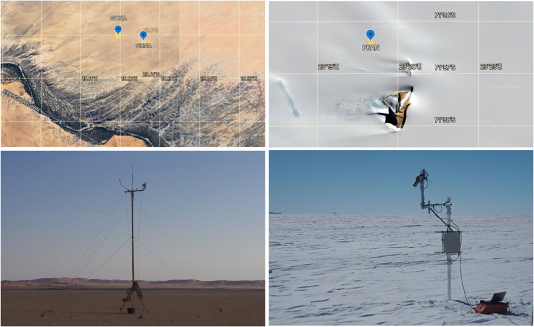
Figure 1. Left: Gobabeb HYPERNETS Namibia (GHNA) Site Location (top) and mast (bottom). Right: Princess Elisabeth Antarctica (PEAN) Site location (top) and mast during the second deployment (bottom).

An example of the GHNA radiance, radiance uncertainty and reflectance is shown in Figure 2. In the bottom panel of this figure, we also show a time series plot showing the temporal stability of the GHNA surface. Only reflectances for one viewing geometry (vza = 5°, vaa = 98°) and wavelength (900 nm) are shown but results for other geometries and wavelengths are also stable. The colour coding shows that there are some differences between the reflectances at different times due to BRDF effects. We also note that the later sequences (14:00-16:00 UTC) show more variability due to the low zenith angle. The measurements used in this study are all in the 8:00-10:00 UTC time window, which are very stable. We also note that the shaded points in the plot show outliers which have effectively been removed by the HYPERNETS quality checks.

Figure 2

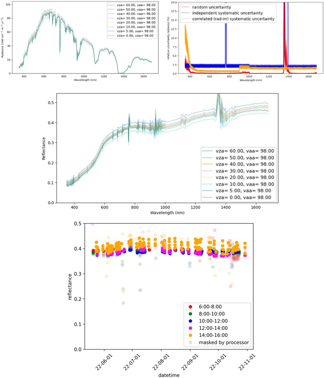
Figure 2. Plots produced by the hypernets_processor for the GHNA site. The radiances (top left), uncertainties (top right) and surface reflectances (centre) on the 2022-06-06 at 09:00 UTC all look sensible. Coloured lines show different viewing zenith (vza) and azimuth (vaa) angles. The bottom panel shows a time series of the 900 nm HYPERNETS measurement for vza = 5°, vaa = 98°, colour-coded by time of day (in UTC, shaded points have not passed the HYPERNETS quality checks). The GHNA site is very stable throughout the deployment.

2.1.2 PEAN

The Belgian Scientific Polar Research Station at Princess Elizabeth Base in Antarctica (PEAN) hosted a HYPSTAR®-XR system between January and March 2022 and between December 2022 and February 2023. This instrument was installed on a mast approximately 2 m above the snow surface (bottom right panel of Figure 1) and operated 24 h per day in temperatures of −5°C to −10°C. The site is located at 71.94013° S, 23.30526° E (top right panel of Figure 1).

The snow surface experiences some change throughout the deployment, mainly as a result of the accumulation of wind-blown snow, and the erosion of the snow surface by the wind. The surface was also affected by shadowing due to the low elevation of the Sun and uneven surface (bottom right panel of Figure 1). The deployment of the HYPSTAR instrument and mast also significantly disturbed the surface for the first deployment. To avoid the worst of the surface disturbance, we do not use the first 2 days after the deployment, to allow wind-blown snow to smooth the surface (which makes a notable difference). During the second deployment, the snow surface was undisturbed. The protocol does not measure in the direction of the access route (trodden snow - Figure 1).

2.1.3 Extracting surface reflectances

BOA surface reflectances at various geometries are available from the HYPERNETS L2A files. All surface reflectance products for GHNA and PEAN that are near simultaneous to a satellite overpass are first downloaded. Examples of the HYPERNETS products are shown in Figures 2, 3 for the GHNA and PEAN data respectively. Surface reflectance measured at the geometry best matching the satellite observation, as well as the associated random and systematic uncertainties, are extracted from the L2A HYPERNETS NetCDF files. For cases where the nearest viewing zenith angle is nadir, the HYPERNETS surface reflectances for the different azimuth angles are averaged.

Figure 3

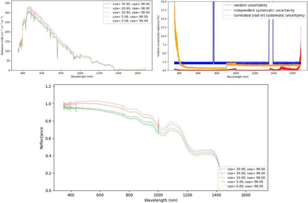
Figure 3. Plots produced by the hypernets_processor for the PEAN site on 2022-01-29 at 07:00 UTC. Coloured lines show different viewing zenith (vza) and azimuth (vaa) angles. The radiances (top left), uncertainties (top right) and surface reflectances (bottom) all look plausible.

2.2 Satellite data

2.2.1 Sentinel-2

The Sentinel-2 (S2) Copernicus mission acquires optical imagery at decametre spatial resolution (10 m–60 m) over land and coastal waters. It consists of two sun-synchronous (polar-orbiting) satellites (S2A and S2B), phased at 180° to each other. S2A and S2B launched in June 2015 and March 2017 respectively. The two satellites together have a revisit time of 5 days at the equator, with shorter revisit times towards the poles. The S2 satellites each carry a multispectral instrument (MSI), which has 13 bands in the visible, near infrared, and short wave infrared part of the spectrum. MSI is a pushbroom scanner with a swath width of 290 km. Radiometric uncertainties for the Sentinel-2 MSI L1C product are available from the Sentinel-2 Radiometric Uncertainty tool (Gorroño et al., 2017), which is part of the ESA SNAP toolbox. A detailed description of S2 together with an S2A performance review is available in (Gascon et al., 2017). A range of papers has investigated the absolute and relative calibration of S2A and S2B and found good radiometric performance to better than 3% for most bands (e.g., Lamquin et al., 2018; Revel et al., 2019).

2.2.2 Landsat 8/9

Landsat 8 (L8) and Landsat 9 (L9) are the two most recent (launched in February 2013 and September 2021 respectively) missions of the NASA/USGS Landsat program, which has been providing satellite imagery of the Earth for more than 50 years. L8 and L9 both have a payload comprised of two instruments, the Operational Land Imager (OLI) and the Thermal Infrared Sensor (TIRS). OLI provides decametre spatial resolution (15-30 m) imagery in the visible, near-infrared and shortwave infrared in nine multispectral bands and TIRS performs thermal imaging in two infrared bands. Both L8 and L9 are in a sun-synchronous orbit with a revisit time of 16 days (at the equator). OLI has a pushbroom scanner with a swath of 185 km. L8 and L9 have been shown to have good radiometric performance to within 3% in reflectance (Markham et al., 2014; Micijevic et al., 2022) and agreement to within 2.5% between L8 and S2 has been demonstrated (Barsi et al., 2018).

2.2.3 PRISMA

PRISMA is a hyperspectral mission by the Italian Space Agency which was launched in March 2019. PRISMA caries a payload of two sensors, the HYC (Hyperspectral Camera) module and the PAN (Panchromatic Camera) module. The HYC sensor is a prism spectrometer with two hyperspectral detectors. The visible/near infrared observed in 66 channels over the spectral interval of 400-1,010 nm, and the near-infrared/shortwave-infrared detector has 171 channels with a spectral interval of 920-2,505 nm. PRISMA is in a sun-synchronous orbit and the HYC has a spatial resolution of 30 m. It is a pushbroom scanner with a swath width of 30 km. The revisit time in nadir view is 29 days, but it is capable of off-nadir observations which can be targeted. The PRISMA radiometric calibration is not as good as S2 and L8, with typical deviations of 5%–7% up to 1800 nm, with a decrease in accuracy in the SWIR (Pignatti et al., 2022).

2.2.4 Identifying match-ups between HYPERNETS and satellite data

A Python tool was developed for identifying match-ups between the HYPERNETS and satellite data. The approach consisted of first downloading all satellite data that covered the GHNA and PEAN sites over the periods for which these sites were operational. The Sentinel-2 (S2) and Landsat 8/9 (L8/9) data were downloaded using the eodag Python package⁴, using the https://earthexplorer.usgs.gov/ repository for Landsat 8/9 and https://peps.cnes.fr/ for Sentinel-2. For PRISMA, data for the appropriate time periods have been manually downloaded from the PRISMA data portal in December 2022 (https://prisma.asi.it/js-cat-client-prisma-src/).

Once the satellite data are downloaded, the Python tool is used to identify the nearest data from the HYPERNETS database to each of the satellite images. Only cloud-free (as identified by HYPERNETS quality checks and/or the satellite masks) match-ups which are found within 1 h of a HYPERNETS measurement are included, with the nearest (in time) HYPERNETS measurement being chosen should there be greater than one HYPERNETS measurement in the time period. Once the match-up is identified, a 200 by 200 m cut-out is made from the satellite image centred on the HYPERNETS site location and stored for further comparison (see Section 3.2).

Limiting the matchups to be within 1 h means that the surface and atmosphere will not vary much between the HYPERNETS and satellite observations. As discussed in Section 2.1.1, the GHNA surface is very temporally stable. This stability means that any uncertainty arising from temporal variation in the surface between the HYPERNETS and satellite measurement is negligible. The PEAN surface is less temporally stable than GHNA due to snow drift, but the temporal variability between the time of the HYPERNETS and the time of the satellite observation is still negligible. The atmospheric parameters are not known exactly (Section 2.3). The uncertainty we include on these parameters also covers any temporal variation they might undergo during 1 h (during clear sky conditions). Finally, the illumination conditions also change with time due to the changing solar zenith angle. We account for this by ensuring to use the solar geometry at the time of the satellite observation when propagating the HYPERNETS measurements to TOA (Section 3.1).

For the GHNA site, there are initially 10 match-ups found with S2 (over 4 months or so), that passed the automated quality checks of the hypernets_processor. Upon further manual quality checks, it was noticed in visual checks of the ‘rgb’ images of the HYPERNETS instrument that for one of the match-ups there was some low fog at the GHNA site. The clear sky quality checks also showed some evidence for this as the irradiance measurements were slightly reduced, but not enough to raise the hypernets_processor clear-sky quality flag. This S2 match-up was also an outlier in terms of the TOA reflectances. As such, this match-up has been manually identified as being of poor quality, and is removed from further analysis, reducing the total number of S2 match-ups over GHNA to 9. Additionally, there are six good quality match-ups with either L8 or L9 and three good quality match-ups with PRISMA within the 1-h match-up window. The total number of match-ups for the GHNA site in this study is thus 18.

For each of the GHNA match-ups, we also check whether RadCalNet data is available within 30 min from the GONA site (located 650 m away from GHNA). GONA data is available for five of the S2 match-ups, three of the L8/9 match-ups and one of the PRISMA match-ups. During the other match-ups, the RadCalNet instrument was not operational. For the nine match-ups with GONA data available, the GONA TOA reflectances are taken directly from the ‘.output’ RadCalNet files. In Section 5.2, we discuss the differences in processing methods between RadCalNet and our own processing. In order to calculate biases between the RadCalNet and satellite data, a separate 200 m by 200 m cut-out is made from the satellite image centred on the GONA site location.

For PEAN, a total of 18 match-ups with valid HYPERNETS data are found in the 1 h window, five match-ups with S2, 13 with L8/9 (after removing outliers with cirrus clouds), and none for PRISMA. It is noted that there are two date (2022-12-27 and 2023-01-12) for which the PEAN site appears in two consecutive tiles for L8/9. In these cases only the matchup where the tile start date is nearest to the HYPERNETS observation is used.

For the two sites combined, we are thus performing comparisons for 36 match-ups between HYPERNETS and the three satellites in this study. A full record of the match-ups is provided in Tables 1, 2 for GHNA and PEAN respectively, including time of observations and respective viewing and solar angles. Plots for each of the match-ups are given in Supplementary Material.

Table 1

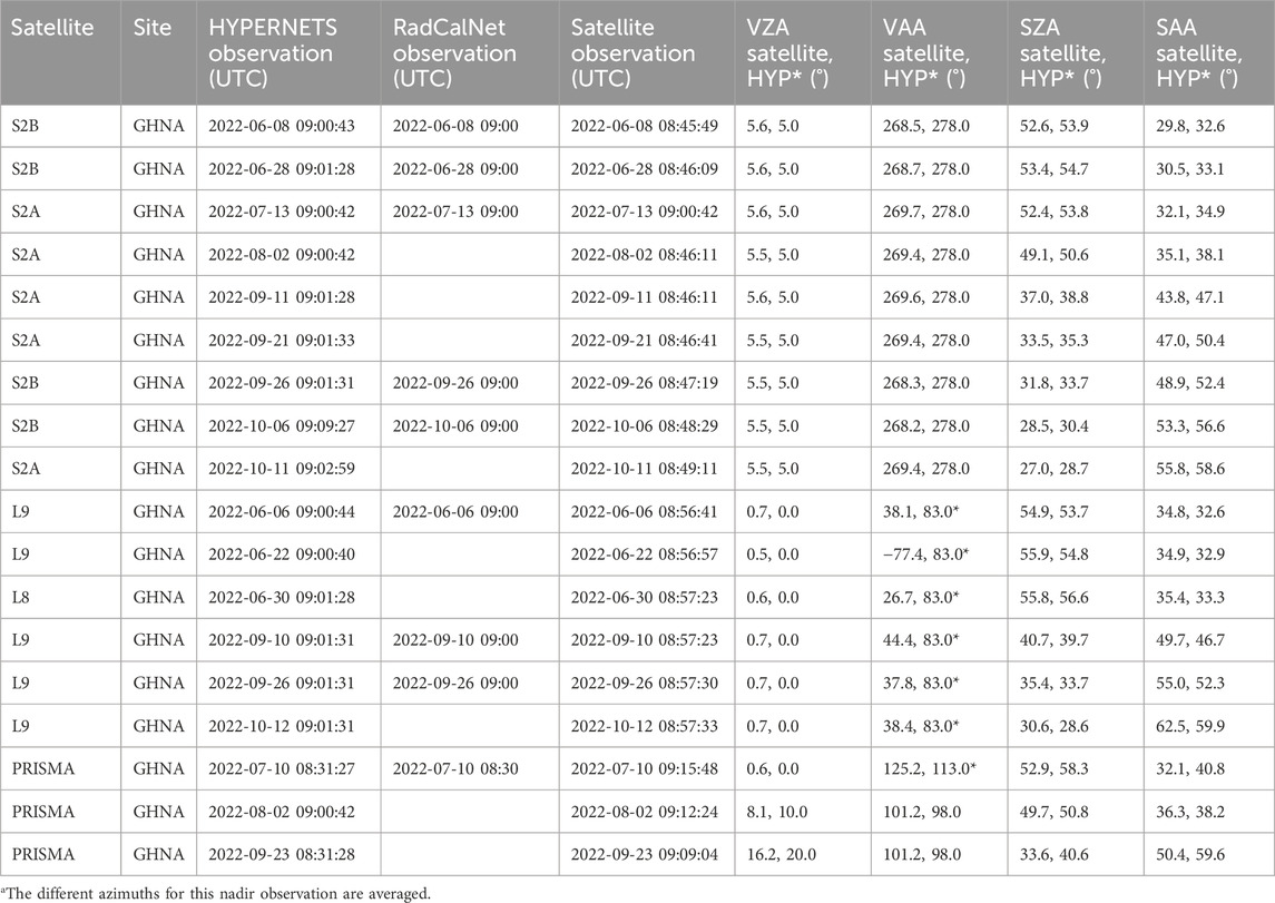
Table 1. Details of all the match-ups between the HYPERNETS data observations for GHNA with the three satellites, including time of measurements, and the viewing and solar zenith and azimuth (measured clockwise from north) angles from the satellite and HYPERNETS (separated by comma in same column).

Table 2

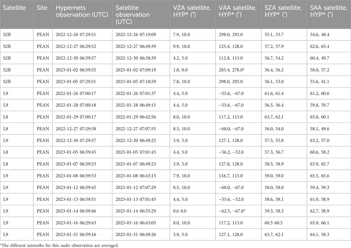
Table 2. Details of all the match-ups between the HYPERNETS data observations for PEAN with Sentinel-2 and Landsat 8/9, including time of measurements, and the viewing and solar angles from the satellite and HYPERNETS (separated by comma in same column).

2.3 Atmospheric data

During the atmospheric propagation process (see Section 3.1), radiative transfer models will be run which take a number of atmospheric parameters as input (specifically aerosol optical depth at 550 nm τ_AOD, aerosol Angstrom component α, total column water vapour TCWV, ozone column density O₃ and pressure p).

For the 9 GHNA match-ups where GONA data is available, τ_AOD, α, TCWV, O₃, p and their uncertainties are all readily available from the RadCalNet GONA data. However, RadCalNet data are not available for all dates for which there are match-ups between GHNA and the satellites. Therefore, we also use ERA5 data (Hersbach et al., 2020) and AERONET (version 3) (Sinyuk et al., 2020) or CAMS (Inness et al., 2019) data. The ERA5 data are downloaded from the Climate Data Store⁵ for TCWV, O₃ and p, with the parameter values taken from the ensemble mean and uncertainties from the ensemble spread. For τ_AOD and α, data for the AERONET Gobabeb site (23.562° S, 14.041° E) are downloaded from the AERONET website⁶. CAMS data are downloaded from the Atmospheric Data Hub⁷ for dates in October 2022 when AERONET data are not available. Results for both types of atmospheric parameters (RadCalNet and ERA5+AERONET/CAMS) are available in Supplementary Figures S1, S2, S4, S5.

PEAN is not a RadCalNet site, and we instead use a combination of either AERONET or CAMS (when AERONET is not available) for τ_AOD and α and ERA5 for TCWV, O₃ and p data. The AERONET data are downloaded from the AERONET website for the Utsteinen site (71.950° S, 23.333° E), which is 1.6 km from the PEAN site. CAMS data are extracted when AERONET data are not available on a given day. For ERA5 (Hersbach et al., 2020), the reanalysis data for the appropriate days were downloaded from the Climate data store. We then extracted the data for the nearest grid point (72.00°S, 23.25° E) at the nearest time. The parameter values were taken from the ensemble mean and the uncertainties from the ensemble spread.

3 Methodology

3.1 Atmospheric propagation

Vicarious calibration of satellites relies on realistic atmospheric propagation of surface reflectances to TOA. In order to determine how much light reaches the TOA, it is necessary to solve the radiative transfer equation, taking into account all the interactions light has with all the atmospheric constituents and the surface (e.g., Rayleigh scattering, aerosol scattering, water vapour absorption, …). The best tools to solve this equation are numerical Radiative Transfer (RT) models. In this section we will provide details on how we performed the atmospheric propagation using the libRadtran RT software package (Emde et al., 2016). We use a metrological approach, where we start by defining a measurement function for the atmospheric propagation and then specify its input quantities in Section 3.1.2.

3.1.1 Atmospheric propagation measurement function

The libRadtran RT software package contains multiple solvers for the RT equation. For this work, we use the 1-dimensional pseudo-spherical DISORT solver, which has been shown to be fast and reliable (Emde et al., 2016). LibRadtran can be set up using a wide range of parameters to define the atmosphere, geometry and processing options. In order to automatically create input files and run the RT models, we have made a Python package, named forts, which among other things, is a wrapper for the libRadtran functionality.

One big advantage of this approach is that we can define a Python version of the measurement function for the atmospheric propagation:

$L_{\text{TOA}}=f\left({\text{ρ}}_{\text{HYPERNETS}},{\tau }_{\text{AOD}},\alpha ,TCWV,{\mathrm{O}}_3,\text{p}\right)+0(2)$

Where L_TOA is the full-resolution TOA RT model for radiance, ρ_HYPERNETS is the surface reflectance from the L2A HYPERNETS product, τ_AOD is the aerosol optical depth at 550 nm, α is the aerosol Angstrom component, TCWV is the total column water vapour, O₃ is the total column ozone and p is the surface pressure. The +0 term is added to indicate this measurement function is an approximation and that there will be errors associated with this approach (in line with the QA4EO guidelines⁸). There are many more parameters that need to be defined in order to fully describe the RT model. However, by defining the measurement function in this way, we can follow a metrological approach when propagating the uncertainties, and use ρ_HYPERNETS, τ_AOD, α, TCWV, O₃ and p as input quantities for which we have uncertainties. The input quantities listed in Eq. 2 are thus the only ones for which we intend to propagate uncertainties. All other inputs to the RT model are hidden within the measurement function f. A Python equivalent of this measurement function is implemented using the forts package, which enables numerical uncertainty propagation, as described in Section 3.3.

3.1.2 Atmospheric propagation parameters

In this section we describe the various inputs to the RT models. We will start with the input quantities for which we propagate uncertainties. ρ_HYPERNETS is taken from the L2A HYPERNETS products for the viewing geometry that most closely matches the satellite geometry. The L2A products also give the random and systematic uncertainties as well as error-correlation matrices for the surface reflectances. The atmospheric datasets used are described in Section 2.3, and also provide uncertainties, which are assumed to have a random error-correlation with respect to each-other.

The following parameters are also set up as part of the radiative transfer model:

• Standard atmosphere: As a starting point, the vertical profiles of all gasses are set to one of the standard atmospheres implemented in libRadtran (cut-off to the input pressure). We use “midlatitude_summer” as the standard atmosphere for our models.

• Solar spectrum: The TSIS solar spectrum at 1 nm resolution (0.1 nm sampling) from Coddington et al. (2021) is used as the extra-terrestrial irradiance. See end of Section 3.3 for a note on the TSIS uncertainties.

• Geometry: The solar zenith angle and solar azimuth angle are calculated for the time and date of the overpass using the pysolar Python package. The viewing zenith and azimuth angle are known from the satellite files.

• Wavelength range: The wavelength range is chosen to be from 380–1,680 nm, based on the availability or HYPERNETS data.

• Wavelength resolution: The RT simulation is run at the resolution of the coarse REPTRAN (Gasteiger et al., 2014) molecular absorption parameterization, which corresponds to a bandwidth of 15 cm⁻¹ when expressed in wavenumber. This corresponds to bandwidths of 0.23 nm in the UV part of the spectrum and increases up to 4 nm for the wavelength around 1700 nm. This is fine enough to get a good sampling of the spectral response function of the various satellites. The spectral sampling is set to 0.1 nm.

• Aerosol properties: Aerosol profiles and optical properties based on size distribution parameters and refractive indices are taken from the “desert” aerosols in the OPAC database (Hess et al., 1998).

The standard atmospheres and “desert” aerosols are thus set up first, and then modified by changing the total aerosol optical depth τ_AOD, aerosol Angstrom component α, total column water vapour TCWV, ozone column density, O₃ and surface pressure p. This allows us to fully define the atmosphere with only few parameters, although this does require assumptions/approximations (mainly that the vertical profiles are known and unchanging and that the aerosol type is represented by a desert aerosol).

3.2 Spectral integration

Before comparing the TOA radiances from the RT models to the satellite observations, they need to be spectrally integrated over the satellite Spectral Response Function (SRF). We use the matheo⁹ Python package, which was developed at NPL for this type of spectral integration and other mathematical algorithms for EO. The Sentinel-2 and Landsat 8 SRFs are available through the pyspectral Python package¹⁰. The matheo package first interpolates the (ir)radiances from the RT model to the wavelengths of the SRF (if the SRF has the highest resolution) or interpolates the SRF to the RT wavelengths (if the RT has higher resolution). It then performs a numerical integration using the composite trapezoidal rule to get the band radiances.

Using matheo, it is possible to define an additional measurement function f₂:

$L_{\text{band,HYPERNETS}}=f_2\left(L_{\text{TOA}},{\xi }_{\text{SRF}}\right)+0(3)$

where L_{band, HYPERNETS} are the band-integrated TOA radiances and L_TOA are the full resolution (0.1 nm sampling) TOA radiances from Eq. 2, and ξ_SRF is the spectral response function for the corresponding satellite band. We then also band-integrate the extra-terrestrial irradiance models E_TOA to the same bands:

$E_{\text{band,HYPERNETS}}=f_2\left(cos\left({\theta }_{\mathit{sun}}\right)E_{\text{TOA}},{\xi }_{\text{SRF}}\right)+0(4)$

where E_{band, HYPERNETS} are the band-integrated downwelling TOA irradiance, θ_sun is the solar zenith angle, E_TOA is the TSIS extraterrestrial irradiance (0.1 nm sampling) and ξ_SRF is the spectral response function for the corresponding satellite band.

The band-integrated radiances (from Eq. 3) and irradiances (from Eq. 4) can then be combined into reflectance (or rather the Hemispherical-directional Reflectance Factor):

${\rho }_{\text{band,HYPERNETS}}=\pi \frac{L_{\text{band,HYPERNETS}}}{E_{\text{band,HYPERNETS}}}(5)$

The resulting band reflectances can directly be compared to the satellite observations ρ_sat. The relative difference, also called bias, δ can be calculated as:

$\delta =\frac{{\rho }_{\text{sat}}}{{\rho }_{\text{band,HYPERNETS}}}-1(6)$

where ρ_{band,HYPERNETS} are the band-integrated TOA reflectances from Eq. 5 and ρ_sat are the observed TOA satellite reflectances.

3.3 Uncertainity propagation

To propagate uncertainties in this work, we use a Monte Carlo (MC) approach (see Supplement one to the “Guide to the expression of uncertainty in measurement”, BIPM et al., 2008), implemented in the punpy Python package. The punpy module is part of the NPL-developed open-source CoMet toolkit (www.comet-toolkit.org). punpy is a Python software package to propagate random, structured and systematic uncertainties through a given measurement function. It has implementations for both the law of propagation of uncertainties and MC methods. For further info on punpy, we refer to De Vis & Hunt (in prep.) or the punpy ATBD¹¹. By defining the atmospheric propagation as a measurement function which has an equivalent Python function, as done in Sections 3.1, 3.2, it is straightforward to propagate uncertainties through this measurement function. We use the MC approach here, because for a numerical measurement function such as ours, this requires much less computing power.

We use 100 MC steps to determine the uncertainties on the TOA band reflectances from the known uncertainties on the input quantities. The uncertainties are determined from the standard deviation in the spread between the 100 MC draws.

When propagating uncertainties in this way, we separate the uncertainties in three contributions:

• Random uncertainties on surface reflectance: These come directly from the L2A HYPERNETS file and are mainly due to noise in the measurements. The errors associated with these uncertainties are entirely uncorrelated. There is no correlation with respect to wavelength, nor with respect to different measurements.

• Systematic uncertainties on surface reflectance: These come directly from the L2A HYPERNETS file and are due to a range of different uncertainty contributions in the calibration of the HYPSTAR^® instruments (such as uncertainties on the calibration distance, alignment, non-linearity, wavelength, lamp and panel). Within these L2A files, the errors associated with these uncertainties are entirely correlated between all different HYPERNETS measurements of that instrument (until the next calibration of that HYPSTAR^® instrument). This means that the errors arising from this component will also be correlated between various match-ups for the same HYPERNETS site. This does not immediately affect the results in this report, but will become important when studying time-series of match-ups. With respect to wavelength, these systematic uncertainties on the surface reflectances have a custom error-correlation, provided as a separate error correlation matrix in the L2A files. This error-correlation will be propagated through the uncertainty propagation. The inclusion of this error-correlation information has a significant effect on the final band-integrated uncertainties, as we will show in Section 4.1.

• Atmospheric uncertainties: The uncertainties on the atmospheric parameters come from the RadCalNet, AERONET, ERA5 and CAMS datasets. RadCalNet has uncertainties available in all files, ERA5 has an ensemble that can be used to determine uncertainties, for AERONET an AOD uncertainty of 0.02 was used (Sinyuk et al., 2020), and for CAMS the AOD uncertainty was set to 10%. The atmospheric parameters are single values, and there is thus no error correlation with wavelength to define. The error-correlation between different match-ups will likely be random as the atmospheric parameters vary on much shorter timescales. We also assume the error-correlation between the different atmospheric parameters is random.

These three uncertainty components are propagated separately, and then combined in quadrature. It is important to propagate these uncertainties separately because for the systematic uncertainties, the covariance between the various wavelengths has to be taken into account. Taking into account the covariances will result in larger uncertainties on the band-integrated radiances compared to treating them as random (see Section 4.1).

For the SRF, no uncertainties are available from pyspectral and we thus neglect these uncertainties. The extra-terrestrial solar irradiances from Coddington et al. (2021) have (k = 1) uncertainties of 0.3% between 460 and 2,365 nm and 1.3% at wavelengths outside that range. However, any error in the irradiance will also affect the radiances in the same manner and will largely cancel out in the reflectances. We thus do not propagate these uncertainties to our TOA reflectances.

There are also uncertainties on the satellite data themselves. There are a range of random (e.g., noise), systematic (e.g., calibration errors) and structured (e.g., straylight) uncertainty components that affect the satellite data. However, a detailed analysis of these for each of the sensors under study is outside the scope of this work. Instead, we used a much simplified uncertainty budget with a random uncertainty component, defined as the standard deviation between the pixels in our cut-out, and a systematic uncertainty component. The errors for this systematic component are assumed to be fully correlated and the uncertainties are set to 3% for S2 and L8/9 and 6% for PRISMA (following radiometric performance assessments detailed in Section 2.2).

Finally, it is worth noting that there are a range of wavelength-dependent model errors (such as any errors present in the RT model itself, the aerosol model used, the vertical profiles assumed, …) for which we have not included an uncertainty contribution (as quantifying these is very difficult and outside the scope of the current study).

4 Results

4.1 Uncertainty budget

As shown in Figure 4, the GHNA and PEAN surfaces have quite different spectral shapes, and different proportions of the TOA reflectance originating in the atmosphere (light directly scattered by the atmosphere without ever interacting with the surface, i.e., the path reflectance). For each match-up, the random and systematic uncertainties on the HYPERNETS surface reflectances and the atmospheric uncertainty are propagated to the TOA HYPERNETS reflectances. These uncertainties are computed for both the full-resolution RT model for the HYPERNETS data as well as for the band integrated models, as is shown in Figure 4 for the GHNA Sentinel-2B match-up on 2022-06-08 and the PEAN Landsat 9 match-up on 2022-01-29. These results are representative for both Sentinel-2 and Landsat 8/9 match-ups. For both cases, the systematic uncertainties are the dominant source of uncertainty at most wavelengths, with smaller contributions for the random and atmospheric uncertainties. It is noted that in the absorption features, there is a greater contribution from the other uncertainties, notably the atmospheric uncertainties. These wavelengths are not suitable for vicarious calibration due to the low gas transmission, but are included here for completeness.

Figure 4

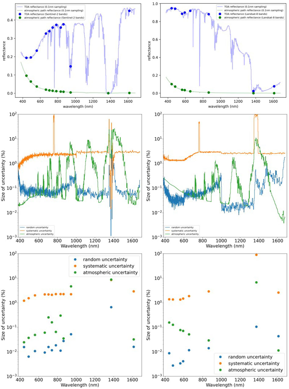
Figure 4. The top row shows the total TOA reflectance together with the atmospheric path reflectance for the GHNA Sentinel-2B match-up on 2022-06-08 (left) and the PEAN Landsat 9 match-up on 2022-01-29 (right). The different uncertainty components (in percent) of the full-resolution RT model are shown in the middle row and the band integrated TOA HYPERNETS uncertainties are shown in the bottom row. The systematic uncertainty dominates the uncertainty except in the atmospheric absorption features.

When the models are band integrated, it is seen for most bands that the systematic and atmospheric uncertainties stay more or less the same as for the full-resolution model. The random uncertainties are significantly reduced by the process of integrating over the spectral response function, following the expected behaviour of scaling with the inverse of the square root of the number of channels being integrated over. For both the Landsat 9 match-up and the Sentinel-2 match-up, the resulting band-integrated uncertainties are again dominated by the systematic uncertainty. For Landsat 9, the B9 band is dominated by the atmospheric uncertainty, as are the B09 and B10 bands for Sentinel-2, as these bands are found in absorption features. The systematic uncertainties (and thus the total uncertainties as well) on the TOA HYPERNETS reflectances are typically slightly larger than the systematic radiometric uncertainties of Sentinel-2 and Landsat 8/9, but smaller than the PRISMA uncertainties.

4.2 GHNA

4.2.1 Sentinel-2

Observations of the TOA reflectance from S2, and from the HYPERNETS data propagated to the TOA follow a similar pattern, which is nearly the same for each of the match-ups as the sites used are radiometrically stable. When RadCalNet data is available, the results between HYPERNETS and RadCalNet TOA reflectances also match well. An example for GHNA (match-up on 2022-06-08) is shown in Figure 5, and similar plots for the full record of match-ups are provided in Supplementary Figures S1–S3. GHNA has TOA reflectances of roughly 0.2 in the visible region, increasing to the region of 0.35–0.4 in the NIR and SWIR. Atmospheric absorption also affects both sets of reflectances, in particular in the 900 and 1,380 nm regions for both S2 and HYPERNETS (the B09 and B10 bands), in addition to the 1,100 nm region for HYPERNETS, as is seen in the top figure of Figure 5, for the 2022-06-08 match-up.

Figure 5

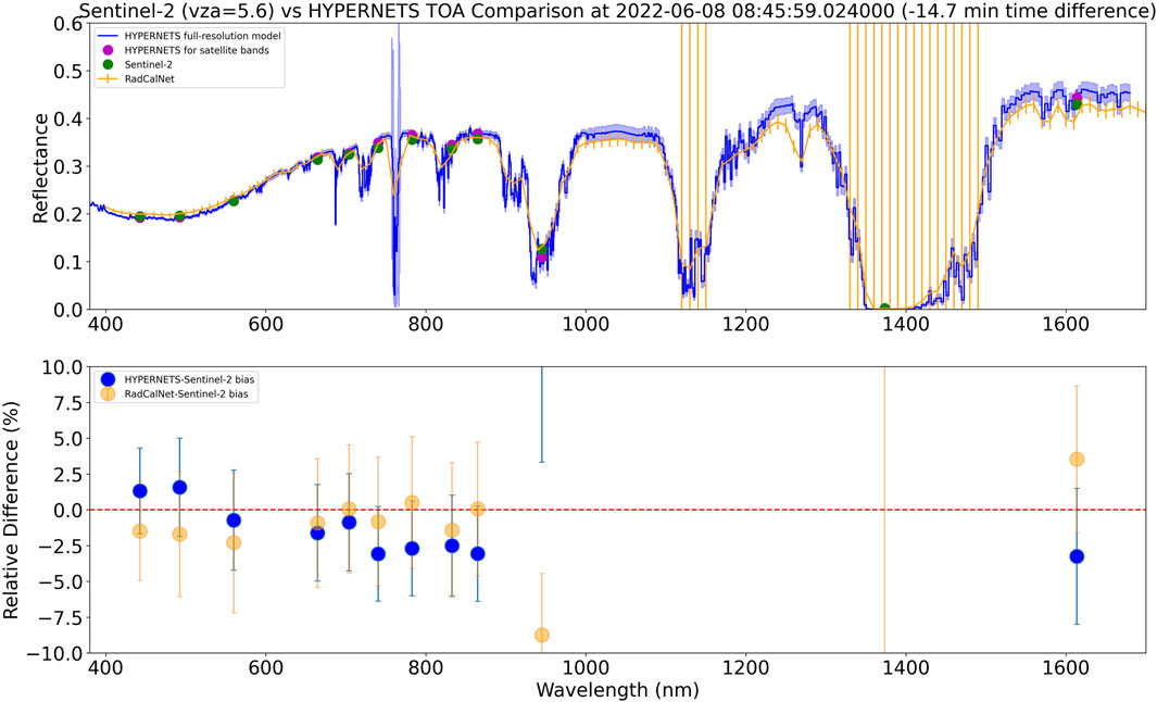
Figure 5. Top: The full-resolution and band-integrated HYPERNETS data compared to Sentinel-2 data and GONA RadCalNet data for the GHNA match-up on 2022-06-08. Shaded area represents uncertainties of HYPERNETS TOA reflectances. Bottom: The percentage difference bias δ between S2 data over GHNA and the band-integrated HYPERNETS data, and between the S2 data over GONA and the RadCalNet TOA reflectances. A few points are off the percentage graph due to the absolute values in reflectance being very small.

For each of the S2 bands, the bias δ (Eq. 6) between the Sentinel-2 and band integrated HYPERNETS data for each Sentinel-2 band is calculated and plotted in the figures as a percentage. For the 2022-06-08 match-up, shown in the bottom of Figure 5, this difference is less than 4% for much of the wavelength range, but is much greater for in the absorption features for bands B09 and B10, where the reflectances are lower due to the absorption. In absolute terms, the bias for B09 and B10 is fairly small. The uncertainties at k = 1 (68% confidence interval), are either consistent with zero (error bars cross zero), or fairly close to it for nearly all bands. For the absorption bands, our placeholder values for the uncertainties are likely underestimated. When inspecting the results for other match-ups in Supplementary Figures S1–S3, we find a similar pattern generally holds. Interestingly, a similar spectral pattern in the bias shows up for most of the match-ups. We will further discuss these differences in Section 5.1.

When the HYPERNETS GHNA biases are compared to those for RadCalNet GONA, we find in some cases RadCalNet GONA has smaller biases, while in others HYPERNETS GHNA has smaller biases. More match-ups would be required to draw robust conclusions, but initial results indicate the GHNA site has similar performance to the GONA site. Further differences between GHNA and GONA are discussed in Section 5.2.

Next, we study whether there is any temporal variation within the nine match-ups between S2 and HYPERNETS. The percentage difference (bias) for all match-ups are plotted as a time series in Figure 6. For this plot, in the propagation of the HYPERNETS data to TOA we used atmospheric properties from ERA5 and AERONET/CAMS for all match-ups for consistency (as opposed to using RadCalNet atmospheric properties when available). For most dates for which there is a match-up between S2 and HYPERNETS at GHNA, each band has a similar bias, showing that the patterns between S2 and HYPERNETS are constant with time. This lack or trend means that during this short 4 month period, there is no notable degradation (which means there is no accumulation of dust, etc., on the HYPERNETS/HYPSTAR^® instrument).

Figure 6

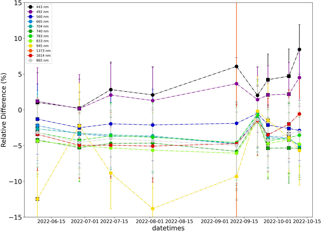
Figure 6. Time series of the percentage difference in S2 data and band-integrated HYPERNETS data for TOA reflectance for the 8 S2-HYPERNETS GHNA match-ups. To propagate the HYPERNETS data to TOA, atmospheric properties from ERA5 + AERONET/CAMS have been used for all match-ups for consistency. S2B results have a black square behind the circles, whereas S2A results are simply circles.

Longer time series would be required to draw any definitive conclusions or to infer anything about the degradation of the satellite. The constant offset also means that these differences are caused by an unchanging effect. This type of offset is likely caused by either a systematic difference in the atmospheric properties, in the calibration, or a systematic difference in how the measurements are made (e.g., misalignment). We note (see also Section 5.2) that the biases are smaller when the RadCalNet atmospheric properties are used.

4.2.2 Landsat 8/9

Landsat 8/9 observations of the TOA reflectances over GHNA, the propagated HYPERNETS data and the RadCalNet TOA data follow a similar pattern to the Sentinel-2 data in the previous section, as well as similar to each other. An example spectrum for the 2022-06-06 match-up and the associated biases are shown in Figure 7. For the 6 Landsat 8/9 match-ups, the percentage difference between them are generally less than 5%, for most of the Landsat 8/9 bands, as is seen in the bottom panel of Figure 7. The B9 band is the exception to this, as this is around the 1,380 nm absorption features, so the reflectances here are lower (resulting in larger percentage difference in spite of reasonable small absolute uncertainties), similar to band B09 and B10 for Sentinel-2. The results for the other match-ups, shown in Supplementary Figures S4–S6, are all quite similar, with biases below 5% for most bands, and consistent with zero within the uncertainties.

Figure 7

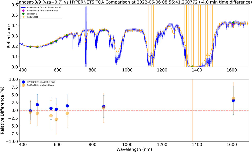
Figure 7. Top: TOA reflectances for the Landsat 9 data and the full-resolution and band-integrated HYPERNETS data, and RadCalNet data for the PEAN match-up on the 2022-06-06. Shaded area represents uncertainties of HYPERNETS TOA reflectances. Bottom: The bias δ (in percentage) between the Landsat 9 data over GHNA and the band-integrated HYPERNETS data, and between the Landsat 9 data over GONA and the RadCalNet TOA reflectances.

The timeseries for all six of the Landsat 8/9 observations is shown in Figure 8, and the differences for all bands apart from B9, mostly being below 5% for all dates. The exception to this is the October match-up is in the region of 8%-10% for B1 and B2. As for the Sentinel-2 match-ups, this increase in the size of the difference could be due to using CAMS data for the aerosol optical depth rather than AERONET data¹² (though this would not affect the larger wavelengths as much).

Figure 8

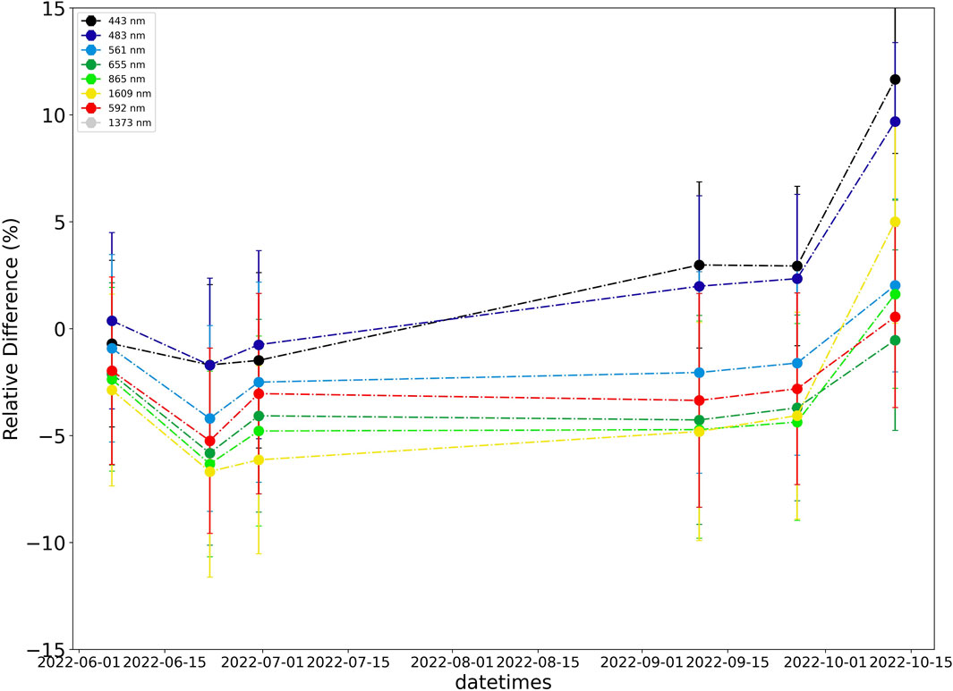
Figure 8. Timeseries of percentage difference for TOA reflectance for the band-integrated HYPERNETS data and Landsat 8/9 observations for the six match-ups at the GHNA sites. To propagate the HYPERNETS data to TOA, atmospheric properties from ERA5 + AERONET/CAMS have been used for all match-ups for consistency.

4.2.3 PRISMA

Finally, we compare the match-ups found between PRISMA and HYPERNETS TOA reflectances. We find good agreement for the GHNA site. Figure 9 shows an example of such a match-up, with differences smaller than 10% for most bands, consistent within the uncertainties. In the absorption features, the measurements still agree reasonably well, but the percentage differences are increased due to the low reflectances. Similar differences are found between RadCalNet and PRISMA. From inspecting the TOA reflectances in Figure 9, we see the RadCalNet GONA and HYPERNETS GHNA data agree better with each other than with PRISMA (when using the same atmospheric properties). The other two match-ups are shown in Supplementary Figure S7. Both these match-ups have somewhat smaller biases (|δ| < 7.5%) than the match-up in Figure 9.

Figure 9

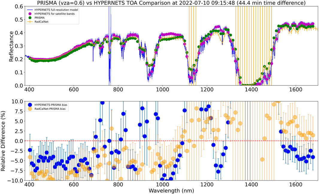
Figure 9. Top: PRISMA reflectances, together with the full-resolution RT model for GHNA, the band-integrated TOA HYPERNETS reflectances, and RadCalNet Reflectances on 2022-07-10. Bottom: The percentage differences between the PRISMA data over GHNA and the TOA HYPERNETS reflectances, and between the PRISMA data over GONA and the RadCalNet TOA reflectances.

4.3 PEAN

Next, we discuss the TOA reflectances and biases for the PEAN site. An example for the Landsat-8 match-up for 2022-01-29 is given is given in Figure 10 and figures for all other match-ups are provided in Supplementary Figures S8, S9. This particular match-up performs quite well with the visible and VNIR bands having biases below 5%, with all of them consistent with zero within their k = 1 uncertainties. The SWIR bands perform poorer, but still show small absolute biases.

Figure 10

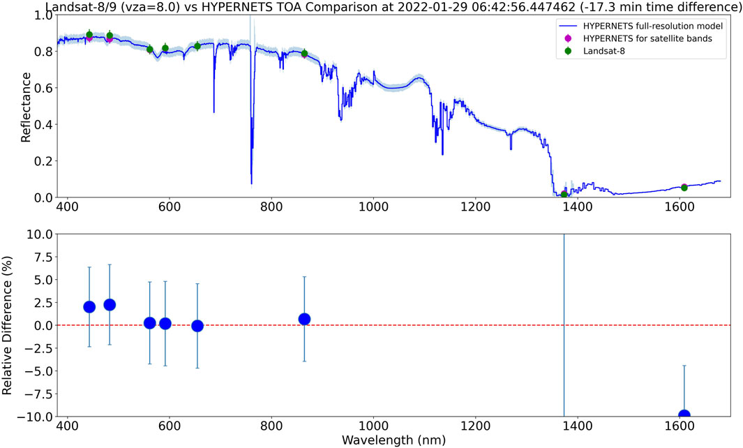
Figure 10. Top: TOA reflectances for the Landsat 8 data and the full-resolution and band-integrated HYPERNETS data for the PEAN match-up on 2022-01-29. Shaded area represents uncertainties of HYPERNETS TOA reflectances. Bottom: The bias δ (in percentage) between the Landsat 9 data and the band-integrated HYPERNETS data.

Even though the example shown in Figure 10 shows that the PEAN site is promising for vicarious calibration, especially given how bright it is, when the other match-ups shown in Supplementary Figures S8, S9 are inspected we find the majority of them perform quite poorly. This is due to variability of the surface on the smaller scales sampled at the 20 cm footprint of the HYPSTAR instrument (due to the mast being only 2 m high). These differences will be further discussed in Section 5.3.

5 Discussions and caveats

5.1 GHNA caveats

The results for GHNA generally perform quite well for each of the different satellites. One potential issue that is revealed when comparing the biases for the different match-ups is that there is a similar spectral pattern, with positive biases (HYPERNETS reflectances smaller than satellite reflectances) in the blue part of the spectrum, but negative biases in the red-VNIR part of the spectrum. The observed biases are mostly within the propagated k = 1 uncertainties, so this is not problematic, but the systematic pattern could indicate an issue either with the calibration, or with the atmospheric correction (either uncertainties on atmospheric properties, or uncertainties in the RT model, see also the caveat about using HCRF in Section 5.4).

Another issue could be that some of the cables or feet holding up the mast, or the solar panel that is mounted on the west leg are in the field of view of the instrument (right panel of Figure 11). In principle the boom on top of the mast is long enough to avoid most of this, but there might be some contamination for certain viewing zenith geometries. In the left panel of Figure 11, we show a polar plot of the surface reflectances at 900 nm for each of the viewing geometries. There is reasonable smooth variability. In future work, we will fit BRDF models to these measurements and check if there are any outliers compared to these models due to contamination by the mast legs or solar panel. If any viewing geometries are affected, these will be masked and replaced by interpolated values. From inspecting the polar plots such as the one given in Figure 11 for each of the match-ups, there is no evidence that the viewing geometries used in the match-ups (indicated by magenta circle) are noticeably affected by this issue.

Figure 11

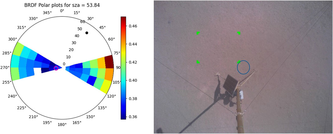
Figure 11. Left: Polar plot showing surface reflectances at 900 nm for different viewing geometries for the GHNA-S2 match-up on 2022-07-13. The solar position is shown as a black dot and satellite viewing geometry as a magenta circle. Right: RGB image taken by the instrument in nadir position. Green box shows the brightest area, which is used to calculate picture exposure. A rough approximation of the field of view is shown as a blue circle.

5.2 Differences between GHNA and GONA

Generally, as shown in Section 4, the agreement between the GHNA HYPERNETS results and GONA RadCalNet results is good (|δ| < 5%). In this section, we investigate the differences between the two sites in a bit more detail. In particular, we investigate variation between the GHNA and GONA surface, differences due to which atmospheric properties are used and differences due to the processing chains used. Each of these are explored for an example Sentinel-2 match-up on 2022-06-28, but similar differences apply for all match-ups.

In Figure 12, we show the percentage differences between the mean TOA reflectances in the GHNA 200 m by 200 m cutout and the GONA 200 m by 200 m cutout, as measured by Sentinel-2 on 2022-06-28. The differences are rather small ($<2$%), indicating the surface at the two sites are consistent with each other.

Figure 12

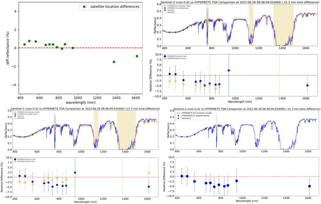
Figure 12. Top left: Differences between the mean Sentinel-2 reflectances on 2022-06-28 in the 200 m by 200 m cutout for GHNA and the cutout for GONA. Top right: Reflectance and bias results HYPERNETS GHNA data (blue), and GHNA (nadir) TOA reflectances processed using the RadCalNet processing chain (orange) for the match-up on 2022-06-28. Bottom: Plots showing the TOA reflecances and biases δ for the Sentinel-2 match-up on 2022-06-28 for the case where RadCalNet atmospheric data is used for the HYPERNETS processing (left) and the case where ERA5+AERONET atmospheric data is used for the HYPERNETS processing (right).

Next we compare the differences due to either using RadCalNet atmospheric properties or those of ERA5 reanalysis data combined with AERONET. In Table 3, we show the extracted atmospheric properties for the Sentinel-2 overpass on 2022-06-28. In Figure 12 (bottom), we show the comparison results for processing the HYPERNETS data using the different sets of atmospheric properties. The results using RadCalNet atmospheric parameters show slightly smaller biases. In Supplementary Figures S1, S2, S4, S5, comparison plots for each Sentinel-2 and Landsat 8 matchup are available for both types of atmospheric parameters. Comparing these results for the different match-ups reveals that generally the performance is slightly better when using RadCalNet atmospheric parameters than when using ERA5+AERONET atmospheric parameters (with even more significant improvement when AERONET is not available and CAMS is used instead).

Table 3

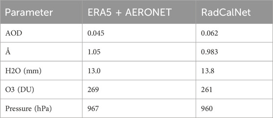
Table 3. Atmospheric properties from ERA5 reanalysis data combined with AERONET, compared to atmospheric properties from RadCalNet.

Finally, we also investigate differences due to the different processing chains. In order to do this, the RadCalNet processing chain has been applied to the GHNA hypernets data. This means that nadir data at GHNA was used, spectrally integrated to the RadCalNet SRF (triangular bands with a width of 10 nm) using matheo, and then processed to TOA by Brian Wenny at NASA (using same methodology as for other RadCalNet sites) using the RadCalNet atmospheric properties. In Figure 12, we show the differences due to these two processing chains for an example by the Sentinel-2 match-up on the 2022-06-28. For this specific example the HYPERNETS processed data results in the smallest biases, but there are other examples where the RadCalNet processing results in smaller biases.

5.3 PEAN variability

Whereas the example for PEAN discussed in Section 4.3 is promising, the additional results shown in the Supplementary Figures S8, S9 show a number of mismatches where the differences were larger than 10%. The differences are in many cases significantly larger than the uncertainties. This is likely because there is significant spatial variability in the PEAN surface reflectances at the scale of the footprint of the PEAN instrument, which is around 20 cm (field of view of 5° on top of 2 m mast). Even though at the spatial resolution observed by satellites ($\ge 10$m) the PEAN surface is very homogeneous, there is significant small-scale variability causes by shadows, as can be seen in Figure 13 (see also the PEAN surface in bottom right panel of Figure 1). This is the result of naturally occurring sastrugi, i.e., small-scale irregularities in the wind-blown snow surface, and their shadows cast by the low Sun.

Figure 13

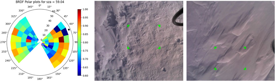
Figure 13. Left: Polar plot showing surface reflectances at 900 nm for different viewing geometries for the PEAN-L8 match-up on 2023-01-07. The solar position is shown as a black dot and satellite viewing geometry as a magenta circle. Middle: RGB image taken by the instrument in nadir position during first deployment. Green box shows the brightest area, which is used to calculate picture exposure. Right: RGB image taken by the instrument in nadir position during second deployment.

The surface continuously changes due to deposition of wind-blown snow and the erosion of the snow surface. This results in an ever changing surface with different patches of shadow. This leads to many of the match-ups shown in Supplementary Figures S8, S9 being of poor quality, but some being good by coincidence. There are both match-ups where the HYPERNETS measurements are overestimated, as well as many where HYPERNETS is underestimated. It is worth pointing out that the small-scale shadowing is also present in the satellite images, yet it is not resolved as a result of the spatial resolution of the satellite sensors. One can thus not simply get rid of any shadow measurements and only use the brightest areas. A more correct approach would be to smooth the data. This cannot be done doing simple averaging over different viewing geometries, as significant BRDF effects are expected for this type of site (Ball et al., 2015). One solution could be to place the instrument significantly higher, though this is likely too challenging in the harsh Antarctic conditions. Another approach would be to fit BRDF models to understand the expected angular behaviour with respect to the observations, and using these BRDF models to smooth the data. Further investigation is required.

In Figure 14, some results are shown for PEAN during observations in cloudy conditions. In these diffuse illumination conditions, the surface variability is much smoother, indicating that the variability observed in Figure 13 indeed results from shadows, and is not caused by instrumental effects. We have discarded any match-ups with cloudy conditions, using the cloud masks of the satellite data to identify them and verifying the presence of clouds by manually inspecting the HYPERNETS sky images. We note that using the HYPERNETS irradiances only, it is hard to identify the cloudy conditions, as the surface is so bright (e.g., multiple surface-atmosphere scattering) and the solar zenith angle is so high (e.g., diffuse cloud scattering combined with cosine response) that the irradiance measurements are sometimes brighter than a clear sky model (Figure 14 right), and as a result the automated HYPERNETS quality checks do not mask these measurements.

Figure 14

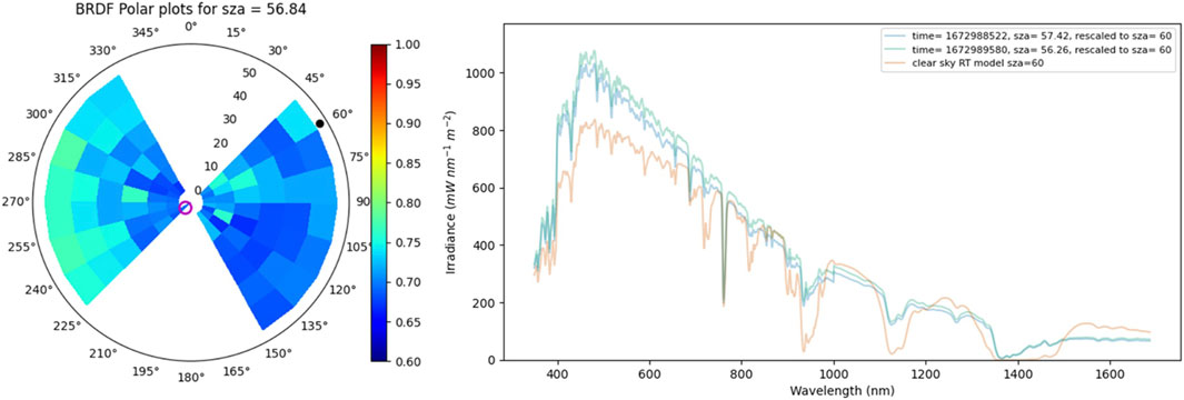
Figure 14. Left: Polar plot showing surface reflectances at 900 nm for different viewing geometries for the PEAN-L8 match-up on 2023-01-06. The solar position is shown as a black dot and satellite viewing geometry as a magenta circle. Right: plot produced by the hypernets_processor which shows its internal quality check comparing the HYPERNETS BOA irradiance measurements to a rudimentary clear sky model. Note that this match-up is not included in Table 2 as it was discarded based on the cloud mask.

One other problem is that due to the low Sun, the irradiance measurements are very sensitive to the allignment of the instrument. Another caveat is that the current methodology for propagating the surface reflectances to TOA is somewhat limited when it comes to modelling PEAN. Due to its high reflectance and BRDF model, there are some combinations of angles that have a directional surface reflectances above 1. While this is not physically impossible, it is currently not possible to use surface reflectances above one in the RT models used in our method.

5.4 General caveats and future work

Even though the biases shown in the previous sections are generally within the uncertainties, there are some bands (especially in the additional examples in the Supplementary Material) for which the biases are significantly larger than the uncertainties. One caveat to this is that our uncertainty budgets are not complete, as we are not including uncertainties on some inputs like the aerosol type, vertical profiles, spatial heterogeneity (at the scale of $\sim 1\text{m}$ footprint for GHNA and $\sim 0.2\text{m}$ for PEAN) etc. The satellite uncertainties could also be improved beyond the simplified random and systematic components we use (e.g., from the S2 RUT tool). Additionally, the HYPERNETS uncertainties not yet include uncertainties accounting for temperature corrections, straylight (placeholder values are used instead) and instrument levelling, which should be added in the future.

As discussed in previous sections, fitting BRDF models would allow us to identify outliers due to contamination and to smooth over small-scale surface variability. More generally, this would also allow us to do a detailed interpolation between the various viewing angles (as opposed to taking the nearest set of angles available from the HYPERNETS measurements), and extend to angles not currently sampled within the measurement sequence. We thus recommend the use of BRDF models in future efforts on vicarious calibration using HYPERNETS data.

In Section 5.2, we discussed the better performance of using RadCalNet GONA atmospheric properties for use in the GHNA processing (which is possible as the sites are only 650 m from each other) as opposed to using reanalysis data such as that from ERA5 and CAMS (AERONET is used for aerosol optical depth when available which is less different from RadCalNet properties). The RadCalNet atmospheric properties use a combination of in situ measurments using a weather station, combined with direct solar measurements to fit the absorption. When the GONA site is down for any reason, no GONA atmospheric data is available and this currently means that GHNA needs to use less reliable reanalysis atmospheric data. However the HYPERNETS measurement sequence does include irradiance measurements, which could also be used for fitting the atmospheric absorption (though both diffuse and direct solar irradiance contributions would need to be taken into account in the fitting). Future studies investigating the use of the HYPERNETS irradiance measurement in combination with weather station data are recommended to derive self-consistent atmospheric properties for GHNA. These atmospheric properties are expected to be of better quality then reanalysis data and will be of most benefit when RadCalNet GONA is not operational for any reason (and thus no GONA atmospheric properties are available). This will also be of significant benefit for the inclusion of the GHNA site into RadCalNet (as GHNA data cannot be included into RadCalNet at times when no reliable atmospheric data is available).

As discussed in Section 2.1, HYPERNETS provides reflectance as Hemispherical-Conical Reflectance Factor (HCRF) instead of the Bi-directional Reflectance Factor (BRF). The BRF is a purely theoretical quantity and cannot be measured directly in the field. However in the radiative transfer simulations, the reflectance is typically expected as BRF. This introduces a small error in the calculated TOA reflectances (few percent for blue wavelengths, reducing for higher wavelengths and negligible for SWIR). This could explain why in our results we typically see more positive biases in the blue bands than for higher wavelengths. In future work we will correct for the HCRF-BRF differences (see, e.g., Schunke et al., 2023).

In this work we have shown that the biases between the HYPERNETS data and Sentinel-2 and Landsat-8/9 are within 5%, and consistent with the uncertainties. Whereas that is a good result that shows the good performance of the HYPERNETS network, this is not a significant improvement (nor is it worse) with respect to previous studies using RadCalNet (Banks et al., 2017; Alhammoud et al., 2019; Jing et al., 2019; Zhao et al., 2021; Murakami et al., 2022). There are a number of areas where further improvement is possible. Some caveats were already discussed above. Another way to improve the study would be to use multiple years of data, over multiple calibration periods, and including various sites. This study is planned in a few years when more data is available. By including more data, it will be possible to average out over any random effects (including random effects that might result in different errors for each calibration period) and to reveal drifts in the calibration.

Another significant improvement would be to make the HYPERNETS data more representative of the satellite measurement. This would mean to better correct for any temporal, spatial and angular differences between the HYPERNETS measurements and the satellite. There are no temporal differences expected in the surface, and changes in illumination are already accounted for, but some improvement could be made from including atmospheric data sampled at higher temporal resolution. Obtaining high resolution imagery over the HYPERNETS sites (either UAV measurements or commercial metre-scale observations from space) would help quantify and correct any spatial differences. Fitting BRDF models would allows to address the angular differences.

6 Conclusion

We have compared a total of 36 satellite images (from Sentinel-2, Landsat 8/9 and PRISMA) to near-simultaneous TOA reflectances for which surface measurements were acquired as part of the HYPERNETS network and processed to TOA. For the GHNA HYPERNETS site, generally good agreement is found, with comparisons with Landsat 8/9 and Sentinel-2 performing well with typical differences smaller than 5%. This performance is similar to that of the RadCalNet GONA site. Comparisons with PRISMA show slightly bigger differences, with typical differences between 0% and 10%. A study comparing the GHNA measurements against a BRDF model and fitting HYPERNETS atmospheric properties is recommended.

The PEAN site also shows good potential for vicarious calibration, with a few match-ups with good agreement to within 5% for Landsat 8/9. However for the majority of match-ups for PEAN the agreement is notable less good (worse than 10%). This is likely due to small-scale variability caused by a wind-blown uneven surface affected by small-scale shadowing. Fitting BRDF models and using these to smooth the data is expected to improve the results.

On the basis on the results presented here the Gobabeb/HYPERNETS site is confirmed as of high interest for vicarious calibration within RadCalNet. The location is already known to be radiometrically stable with good spatial homogeneity and frequent clear sky conditions and there is already a RadCalNet site nearby based on a multispectral radiometer. The added value of HYPERNETS is that the use of a hyperspectral radiometer (with relatively fine spectral resolution, 3 nm FWHM) avoids the need for spectral interpolation/fitting for bands that are not well-covered by the multispectral instrument because wide and/or with wavelengths simply not measured multispectrally. This is particularly important for the new generation of hyperspectral instruments such as ENMAP, PRISMA, EMIT, PACE, SBG, CHIME and GLIMR.

The PEAN/HYPERNETS site, which was originally intended only for validation purposes is revealed here to be relevant also as a new vicarious calibration site, which may be included in RadCalNet. The added value of this site, compared to existing RadCalnet sites, is that: the site has very different surface reflectance from existing sites (very bright for most of the VNIR), ensures that the HYPSTAR instrument is tested in both very hot (Gobabeb) and very cold (Antarctica) conditions and has potentially a large number of match-ups due to the high latitude and long photoperiod in the Southern hemisphere summer. This site also has often a clear atmosphere and benefits from intensive atmospheric measurements, which may help improve the modelling to TOA reflectance. The challenges of this site include the modelling of atmospheric radiative transfer at high Sun zenith angle and the complicated BRDF effects associated with terrain shadowing at high Sun zenith angle. The latter requires extra research, but the multi-angle high frequency HYPERNETS data are ideally suited for improving the understanding of BRDF of snow surfaces and hence potentially the remote sensing of snow properties.

Data availability statement

The raw data supporting the conclusion of this article will be made available by the authors, without undue reservation.

Author contributions

PD: Formal Analysis, Methodology, Writing–original draft, Conceptualization, Investigation, Software, Visualization. AH: Formal Analysis, Visualization, Writing–review and editing. QV: Investigation, Writing–review and editing. AB: Conceptualization, Funding acquisition, Investigation, Project administration, Writing–review and editing. HM: Software, Writing–review and editing. MS: Investigation, Writing–review and editing. KR: Funding acquisition, Project administration, Writing–review and editing.

Funding

The author(s) declare that financial support was received for the research, authorship, and/or publication of this article. The HYPERNETS project is funded by the European Union’s Horizon 2020 research and innovation program under grant agreement No 775983 and by the HYPERNET-POP project funded by the European Space Agency (contract n◦ 4000139081/22/I-EF). This work (and the CoMet toolkit used within) has also received funding from the ESA-funded Instrument Data quality Evaluation and Assessment Service - Quality Assurance for Earth Observation (IDEAS-QA4EO) contract funded by ESA-ESRIN (n. 4000128960/19/I-NS) and the UK’s Department for Business, Energy and Industrial Strategy’s (BEIS) National Measurement System (NMS) programme.

Acknowledgments

We thank the Copernicus program, the U.S. Geological Survey, and the Italian Space Agency for the use of their data, as well as the eodag team for making their tools available. We also gratefully acknowledge Maddie Stedman for her help with the PRISMA data, Mattea Goalen for help with the data readers, Brian Wenny for the GHNA RadCalNet processing and Mohammadmehdi Saberioon for interesting discussion. We gratefully acknowledge Gillian Maggs-Kolling, Eugene Marais, Martin Handjaba and the Gobabeb Research Center team for their support during deployment and servicing of the RadCalNet GONA and HYPERNETS GHNA instruments. We thank Michel Van Roozendal, Alexander Mangold and Alexis Merlaud for their effort in establishing and maintaining the Utsteinen AERONET site and Stuart Piketh and Gillian Maggs-Kolling for their effort in establishing and maintaining the Gobabeb AERONET site. The International Polar Foundation (IPF) and Clemence Goyens are warmly thanked for supporting the PEAN deployment. The HYPERNETS partners, especially Tartu University and Sorbonne University are thanked for technical support and development of the HYPSTAR^® instrument and system. Paul Green is thanked for useful comments.

Conflict of interest

The authors declare that the research was conducted in the absence of any commercial or financial relationships that could be construed as a potential conflict of interest.

Publisher’s note

All claims expressed in this article are solely those of the authors and do not necessarily represent those of their affiliated organizations, or those of the publisher, the editors and the reviewers. Any product that may be evaluated in this article, or claim that may be made by its manufacturer, is not guaranteed or endorsed by the publisher.

Supplementary Material

The Supplementary Material for this article can be found online at: https://www.frontiersin.org/articles/10.3389/frsen.2024.1323998/full#supplementary-material

Footnotes

¹http://calvalportal.ceos.org/cal/val-wiki/-/wiki/CalVal+Wiki/Vicarious+Calibration

²https://HYPERNETS-processor.readthedocs.io/en/latest/?badge=latest

³https://doi.org/10.5281/zenodo.8039303

⁴https://eodag.readthedocs.io/en/stable/

⁵https://cds.climate.copernicus.eu/cdsapp\#!/dataset/reanalysis-era5-single-levels?tab=form

⁶https://aeronet.gsfc.nasa.gov/

⁷https://ads.atmosphere.copernicus.eu/cdsapp\#!/yourrequests?tab=form

⁸https://qa4eo.org/

⁹https://matheo.readthedocs.io/en/latest/

¹⁰https://pyspectral.readthedocs.io/en/master/installation.html\#the-spectral-response-data

¹¹https://punpy.readthedocs.io/en/latest/content/atbd.html

¹²AERONET and CAMS were found to be consistent when both were available, though with larger uncertainties for CAMS.

References

Alhammoud, B., Jackson, J., Clerc, S., Arias, M., Bouzinac, C., Gascon, F., et al. (2019). Sentinel-2 level-1 radiometry assessment using vicarious methods from dimitri toolbox and field measurements from radcalnet database. IEEE J. Sel. Top. Appl. Earth Observations Remote Sens. 12, 3470–3479. doi:10.1109/JSTARS.2019.2936940

CrossRef Full Text | Google Scholar

Ball, C. P., Marks, A. A., Green, P. D., MacArthur, A., Maturilli, M., Fox, N. P., et al. (2015). Hemispherical-directional reflectance (hdrf) of windblown snow-covered arctic tundra at large solar zenith angles. IEEE Trans. Geoscience Remote Sens. 53, 5377–5387. doi:10.1109/TGRS.2015.2421733

CrossRef Full Text | Google Scholar

Banks, A. C., Hunt, S. E., Gorroño, J., Scanlon, T., Woolliams, E. R., and Fox, N. P. (2017). “A comparison of validation and vicarious calibration of high and medium resolution satellite-borne sensors using radcalnet,” in Sensors, systems, and next-generation satellites XXI. Editors S. P. Neeck, J.-L. Bézy, and T. Kimura (United States: International Society for Optics and Photonics), 10423. doi:10.1117/12.2278528

CrossRef Full Text | Google Scholar

Barsi, J., Alhammoud, B., Czapla-Myers, J., Gascon, F., Haque, M., Kaewmanee, M., et al. (2018). Sentinel-2A MSI and Landsat-8 OLI radiometric cross comparison over desert sites. Italian J. Remote Sens./Rivista Italiana di Telerilevamento 51, 822–837. doi:10.1080/22797254.2018.1507613

CrossRef Full Text | Google Scholar

Bialek, A., Greenwell, C., Lamare, M., Meygret, A., Marcq, S., Lachérade, S., et al. (2016). “New radiometric calibration site located at gobabeb, namib desert,” in 2016 IEEE International Geoscience and Remote Sensing Symposium (IGARSS), Beijing, China, July 10-15, 2016, 6094–6097.

CrossRef Full Text | Google Scholar

Bipm, , Iec, , Ifcc, , Ilac, , Iso, , and Iupac, (2008). Evaluation of measurement data — guide to the expression of uncertainty in measurement. Joint Committee for Guides in Metrology. JCGM 100, 2008.

Google Scholar

Bouvet, M., Thome, K., Berthelot, B., Bialek, A., Czapla-Myers, J., Fox, N. P., et al. (2019). Radcalnet: a radiometric calibration network for earth observing imagers operating in the visible to shortwave infrared spectral range. Remote Sens. 11, 2401. doi:10.3390/rs11202401

CrossRef Full Text | Google Scholar

Coddington, O. M., Richard, E. C., Harber, D., Pilewskie, P., Woods, T. N., Chance, K., et al. (2021). The tsis-1 hybrid solar reference spectrum. Geophys. Res. Lett. 48, e2020GL091709. doi:10.1029/2020GL091709

PubMed Abstract | CrossRef Full Text | Google Scholar

De Vis, P., Bialek, A., and Sinclair, M. (2023). Initial sample of HYPERNETS hyperspectral surface reflectance measurements for satellite validation from the gobabeb site in Namibia. Zendo. doi:10.5281/zenodo.8039303

CrossRef Full Text | Google Scholar

De Vis, P., Goyens, C., Hunt, S., Vanhellemont, Q., Ruddick, K., and Bialek, A. (2024). Generating hyperspectral reference measurements for surface reflectance from the LANDHYPERNET and WATERHYPERNET networks. Front. Remote Sens. 5 ISSN=2673-6187. doi:10.3389/frsen.2024.1347230

CrossRef Full Text | Google Scholar

Emde, C., Buras-Schnell, R., Kylling, A., Mayer, B., Gasteiger, J., Hamann, U., et al. (2016). The libradtran software package for radiative transfer calculations (version 2.0.1). Geosci. Model Dev. 9, 1647–1672. doi:10.5194/gmd-9-1647-2016

CrossRef Full Text | Google Scholar

Gascon, F., Bouzinac, C., Thépaut, O., Jung, M., Francesconi, B., Louis, J., et al. (2017). Copernicus sentinel-2a calibration and products validation status. Remote Sens. 9, 584. doi:10.3390/rs9060584

CrossRef Full Text | Google Scholar

Gasteiger, J., Emde, C., Mayer, B., Buras, R., Buehler, S. A., and Lemke, O. (2014). Representative wavelengths absorption parameterization applied to satellite channels and spectral bands. J. Quantitative Spectrosc. Radiat. Transf. 148, 99–115. doi:10.1016/j.jqsrt.2014.06.024

CrossRef Full Text | Google Scholar

Gorroño, J., Fomferra, N., Peters, M., Gascon, F., Underwood, C. I., Fox, N. P., et al. (2017). A radiometric uncertainty tool for the sentinel 2 mission. Remote Sens. 9, 178. doi:10.3390/rs9020178

CrossRef Full Text | Google Scholar

Hersbach, H., Bell, B., Berrisford, P., Hirahara, S., Horányi, A., Muñoz-Sabater, J., et al. (2020). The era5 global reanalysis. Q. J. R. Meteorological Soc. 146, 1999–2049. doi:10.1002/qj.3803

CrossRef Full Text | Google Scholar

Hess, M., Koepke, P., and Schult, I. (1998). Optical properties of aerosols and clouds: the software package opac. Bull. Am. Meteorological Soc. 79, 831–844. doi:10.1175/1520-0477(1998)079-0831:OPOAAC-2.0.CO;2

CrossRef Full Text | Google Scholar

Inness, A., Ades, M., Agustí-Panareda, A., Barré, J., Benedictow, A., Blechschmidt, A.-M., et al. (2019). The cams reanalysis of atmospheric composition. Atmos. Chem. Phys. 19, 3515–3556. doi:10.5194/acp-19-3515-2019

CrossRef Full Text | Google Scholar

Jing, X., Leigh, L., Teixeira Pinto, C., and Helder, D. (2019). Evaluation of radcalnet output data using landsat 7, landsat 8, sentinel 2a, and sentinel 2b sensors. Remote Sens. 11, 541. doi:10.3390/rs11050541

CrossRef Full Text | Google Scholar

Lamquin, N., Bruniquel, V., and Gascon, F. (2018). Sentinel-2 l1c radiometric validation using deep convective clouds observations. Eur. J. Remote Sens. 51, 11–27. doi:10.1080/22797254.2017.1395713

CrossRef Full Text | Google Scholar

Markham, B., Barsi, J., Kvaran, G., Ong, L., Kaita, E., Biggar, S., et al. (2014). Landsat-8 operational land imager radiometric calibration and stability. Remote Sens. 6, 12275–12308. doi:10.3390/rs61212275

CrossRef Full Text | Google Scholar

Micijevic, E., Barsi, J., Haque, M., Levy, R., Anderson, C., Thome, K., et al. (2022). English (US)Radiometric performance of the landsat 9 operational land imager over the first 8 months on orbit. In Earth Observing Systems XXVII. Proc. SPIE - Int. Soc. Opt. Eng. doi:10.1117/12.2634301

CrossRef Full Text | Google Scholar

Murakami, H., Antoine, D., Vellucci, V., and Frouin, R. (2022). System vicarious calibration of GCOM-C/SGLI visible and near-infrared channels. J. Oceanogr. 78, 245–261. doi:10.1007/s10872-022-00632-x

CrossRef Full Text | Google Scholar

Pignatti, S., Amodeo, A., Carfora, M. F., Casa, R., Mona, L., Palombo, A., et al. (2022). Prisma l1 and l2 performances within the priscav project: the pignola test site in southern Italy. Remote Sens. 14, 1985. doi:10.3390/rs14091985

CrossRef Full Text | Google Scholar

Revel, C., Lonjou, V., Marcq, S., Desjardins, C., Fougnie, B., Luche, C. C.-D., et al. (2019). Sentinel-2a and 2b absolute calibration monitoring. Eur. J. Remote Sens. 52, 122–137. doi:10.1080/22797254.2018.1562311

CrossRef Full Text | Google Scholar

Ruddick, K., Brando, V. E., Corizzi, A., Dogliotti, A. I., Doxaran, D., Goyens, C., et al. (2024a). WATERHYPERNET: A prototype network of automated in situ measurements of hyperspectral water reflectance for satellite validation and water quality monitoring. Front. Remote Sens. 5. doi:10.3389/frsen.2024.1347520

CrossRef Full Text | Google Scholar

Ruddick, K. G., Bialek, A., Brando, V. E., De Vis, P., Dogliotti, A. I., Doxaran, D., et al. (2024b). HYPERNETS: a network of automated hyperspectral radiometers to validate water and land surface reflectance (380–1680 nm) from all satellite missions. Front. Remote Sens. 5 ISSN=2673-6187. doi:10.3389/frsen.2024.1372085

CrossRef Full Text | Google Scholar

Schunke, S., Leroy, V., and Govaerts, Y. (2023). Retrieving brdfs from uav-based radiometers for fiducial reference measurements: caveats and recommendations. Front. Remote Sens. 4. doi:10.3389/frsen.2023.1285800

CrossRef Full Text | Google Scholar

Sinyuk, A., Holben, B. N., Eck, T. F., Giles, D. M., Slutsker, I., Korkin, S., et al. (2020). The aeronet version 3 aerosol retrieval algorithm, associated uncertainties and comparisons to version 2. Atmos. Meas. Tech. 13, 3375–3411. doi:10.5194/amt-13-3375-2020

CrossRef Full Text | Google Scholar

Zhao, Y., Ma, L., Li, W., He, H., Long, X., Wang, N., et al. (2021). “Vicarious radiometric calibration of superview-1 sensor using radcalnet toa reflectance product,” in 2021 IEEE International Geoscience and Remote Sensing Symposium IGARSS, Brussels, Belgium, July 11-16, 2021, 8130–8133.

CrossRef Full Text | Google Scholar