Apparent surface-to-sky radiance ratio of natural waters including polarization and aerosol effects: implications for above-water radiometry

Above-water radiometry (AWR) methods have been developed to provide “ground-truth” (or fiducial) measurements for calibration and validation of the water color satellite missions. AWR is also an important tool for environmental survey from dedicated field missions. Under clear sky, the critical step of AWR is to retrieve the water-leaving radiance from radiometric measurements of the upward radiance that also includes the reflection of the direct sunlight and diffuse skylight reflected by the wind ruffled water surface toward the sensor. In order to correct for the surface reflection, sky radiance measurements are performed and converted into surface radiance through a factor often called “sea surface reflectance factor” or “effective Fresnel reflectance coefficient”. Based on theoretical and practical considerations, this factor was renamed surface-to-sky radiance ratio, $R_{ss}$, to avoid misuse of the term reflectance as often encountered in the literature. Vector radiative transfer computations were performed over the spectral range 350–1,000 nm to provide angular values of $R_{ss}$ for a comprehensive set of aerosol loads and types (including maritime, continental desert and polluted models) and water surface roughness expressed in wave slope variances or in equivalent Cox-Munk wind speeds, for practical use. After separating direct and diffuse light components, it was shown that the spectral shape and amplitude of $R_{ss}$ are very sensitive to aerosol load and type even for extremely low values of the aerosol optical thickness. Uncertainty attached to $R_{ss}$ was computed based on propagation of errors made in aerosol and surface roughness parameters demonstrating the need to adapt the viewing geometry according to the Sun elevation and to associate concurrent aerosol measurements for optimal AWR protocols.

1 Introduction

Optical remote sensing has become a critical tool to monitor oceanic, coastal or inland aquatic environments and their inherent ecosystems thanks to multispectral or hyperspectral measurements of the water-leaving radiance $L_w$ (Werdell et al., 2018; Giardino et al., 2019). $L_w$ is conceptually defined as the radiance exiting a water body in a given upward direction after transmission through the water-air interface (Mueller and Austin, 1995), which strictly does not include the radiance of the air-water interface (i.e., sky and Sun reflection on the water surface). Spectral $L_w$ originates from light interaction with matter within the water body and is therefore informative on the nature of the optically active water constituents (OAWC). A series of scientific algorithms, in particular the so-called atmospheric correction, must be applied to the raw satellite measurements in order to retrieve the water-leaving radiance which constitutes a small part of the total signal often dominated by the atmosphere and surface-reflected light. The overall process to retrieve the water-leaving radiance from space-sensors is therefore very sensitive to both the radiometric performance of the sensors (calibration) (Hu et al., 2001; Franz et al., 2007) and the optimality of the radiative transfer modeling and inverse problem methods (Gilerson et al., 2023). Since uncertainties accumulate from sensor calibration to retrieval algorithm application, quantitative evaluation of uncertainty and bias is of paramount importance to help minimize them for a beneficial exploitation of the L_w data for scientific or environmental monitoring activities.

For this purpose, field measurements are efficient tools provided that their own data quality is sufficiently high and that their attached uncertainties are metrologically quantified. Two different systems were installed for quality evaluation of the historical “ocean color” satellite sensors (e.g., MERIS, MODIS, SeaWiFS): in-water and above-water radiometric systems (Hooker et al., 2002; Zibordi et al., 2002). Both systems possess their own advantages and weaknesses regarding either the implementation in the field or data processing for retrieval of L_w at the exact water surface level (denoted as 0⁺). For instance, retrieval of water-leaving radiance from in-water radiometric methods is very sensitive to extrapolation at 0⁺ from the measured underwater profile of the upward radiance (Antoine et al., 2008; Hooker et al., 2013). It is worth noting that for turbid or highly absorbing waters, potentially encountered in coastal or lake environments, in-water methods are impracticable due to rapid loss of light (signal) with depth (e.g., within the first tens of centimeter). As for above-water system, the main issue is to remove the sun and sky light reflected on the water surface. Those inherent difficulties were in part alleviated by the development of dedicated protocols (Mueller and Austin, 1995; Zibordi et al., 2019).

For operational calibration and validation activities of the in-orbit satellite missions, dense time-series are needed to maximize the number of match-up points between reference field measurements and satellite acquisitions. This necessitates the installation of “unattended” radiometric systems with quasi-continuous acquisitions over time. To this end, the AERONET-OC network has been developed since 2002 to provide L_w time-series for open and coastal waters, as well as inland waters, based on an above-water multispectral system (Zibordi et al., 2009). Recently, this network has been complemented by an hyperspectral setup based on the same above-water radiometry procedures (Goyens et al., 2022). In addition to the fixed platforms equipped by those networks, above-water radiometry methods are also deployed on small to big ships including research vessels (Ondrusek et al., 2022), ferries (Nasiha et al., 2022) or even dugout canoes (Marinho et al., 2021) to enable gathering of large amounts of data to document the optical diversity of aquatic environments and consequently help to improve satellite remote sensing capabilities (Pahlevan et al., 2021).

For satellite validation purposes, fiducial measurements are acquired under clear sky conditions, i.e., in absence of clouds in the vicinity. In this case, the water surface is illuminated by the direct sunlight and the diffuse skylight originating from scattering by molecules and aerosols of the overlying atmosphere. Part of this light enters the water body where the radiation is altered through absorption and scattering caused by the water molecules as well as the presence of dissolved and particulate matter. Thus, as already mentioned, the water-leaving radiance carries useful information to estimate parameters related to the OAWC, such as phytoplankton or sediment concentration proxies, and the in-water light regime (e.g., water transparency). The other part is reflected by the wind ruffled air-water interface contributing to the surface component of the upward radiance. The main principle of above-water radiometry (AWR) relies on a couple of measurements: 1) the total radiance coming from the water body and surface measured with an oblique angle (typically 40°), and 2) downward radiance of the direction that would be specularly reflected by a conceptual flat surface toward the sensor used for 1). The second term is converted into the surface radiance to be removed using a factor that should account for the reflection of the air-water interface considering its roughness properties (Mobley, 1999). This factor is usually defined as “a coefficient that represents the fraction of incident skylight that is reflected back towards the water-viewing sensor at the air-water interface and is the Fresnel reflectance coefficient for a flat water surface”, see (Ruddick et al., 2019) where the authors argue to name this term “effective Fresnel reflectance coefficient”. Note that other terms are also found in the literature with, for instance, sea surface reflectance factor (Mobley, 1999) or radiance reflectance factor (Mobley, 2015).

In general, the water surface is “crinkled” by gusts of wind modifying its roughness and in turn its reflection properties (Preisendorfer and Mobley, 1986). The main consequence is that the surface-reflected skylight toward the water-viewing sensor originates from many parts of the celestial hemisphere. This can be understood as a superposition of Fresnel reflections integrated over all the hemispherical directions implying that the “effective Fresnel reflectance coefficient” is sensitive to 1) the wave distribution, including gravitary and capillary waves (Mobley, 2015), 2) the radiance distribution within the celestial dome (Mobley, 1999), 3) the polarization state of light (Harmel, Gilerson, Tonizzo, et al., 2012). These three points should be accounted for in the computation of the “effective Fresnel reflectance coefficient”. The first tabulated values were calculated based on Monte-Carlo method to the radiative transfer equation under a simplified atmosphere and without accounting for polarization (Mobley, 1999). Further computations included polarization effects but for a pure Rayleigh atmosphere (i.e., no aerosol), (Mobley, 2015). Nevertheless, the two kinds of values were evaluated based on an in situ data set showing no significant impact on the L_w retrievals from an AERONET-OC site (Zibordi, 2016). Other studies provided values considering polarization and impact of a few aerosol types (Zhang et al., 2017; Gilerson et al., 2018). The consideration of both polarization and aerosol optical properties enabled the reproduction of the spectral variation of the sky to surface radiance conversion factor observed from the field (Lee et al., 2010; Lin et al., 2023).

It is proposed in this study to expand those computations for all potential viewing geometries for a comprehensive set of air-water interface roughness properties and aerosol types encompassing realistic models for open ocean, coastal, and inland areas (including polluted areas and desert dust). The effects of water surface and aerosol types are taken into account through full vector radiative transfer computations to provide pre-computed tabulated values. The main terms and equations to achieve such computations are detailed in the next section. A specific attention is paid to the nomenclature of the different terms to exemplify possible accordance between theoretical and applicative notations in used in the field of aquatic remote sensing. The uncertainty attached to unknown or partially known input parameters to the modeled values are computed based on Gaussian error propagation. Finally, recommendations to reduce uncertainty in AWR procedures are given based on separate treatment of the diffuse and direct light components, supplementary atmospheric measurements and adaptable viewing geometries.

2 Material and method

2.1 Theoretical background

2.1.1 Radiance components

Above-water radiometry (AWR) methodology mainly relies on (i) radiance measurements performed with a sensor pointed downward to the water, L_t, (ii) measurements of the sky radiance, $L_{sky}$, with a radiometer pointed to the direction that would be specularly reflected by a conceptual flat surface toward the sensor used for (i), and (iii) correction of the skylight reflected onto the water surface and reaching the downward looking sensor. For the sake of brevity, the impact of the field-of-view of the sensor is not considered in the angular notation below. Assuming the water body and the air-water interface as two different layers, the total radiance measured by the sensor pointing downward can be decomposed as follows:

$L_t\left({\theta }_s,{\theta }_v,\Delta \varphi ,\lambda \right)=L_w\left({\theta }_s,{\theta }_v,\Delta \varphi ,\lambda \right)+L_{surf}\left({\theta }_{\text{s}},{\theta }_v,\Delta \varphi ,\lambda \right),(1)$

where θ_s and θ_v are the sun and viewing zenith angles, $\Delta \varphi$ is the relative azimuth between the sun and the direction of the radiometer, the angle convention is given in Figure 1, λ is the wavelength. L_t, L_w and L_surf are the total, the water-leaving and the surface (reflected skylight) radiances, respectively. The remote sensing reflectance is obtained after dividing L_w by the downwelling irradiance. It is important to note that the three angles (θ_s, θ_v, $\Delta \varphi$) must be considered due to the anisotropic nature of the radiation components L_t, L_w and L_surf. Note that floating material or foam and white caps are not considered in Eq. 1. A glossary of the main symbols is given in Table 1.

FIGURE 1

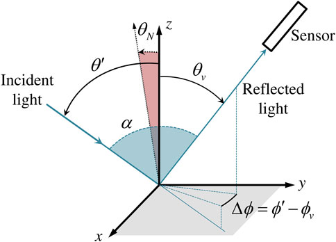
FIGURE 1. Viewing geometry convention: ${\theta }_v$ and ${\varphi }_v$ are the zenith angle and azimuth of the viewing direction, ${\theta }^{\prime }$ and ${\varphi }^{\prime }$ are the zenith angle and azimuth of a given illumination direction. ${\theta }_N$ is defined as the zenith angle of the vector normal to a given wave facet, and $\alpha$ is the phase angle between the incident and viewing directions.

TABLE 1

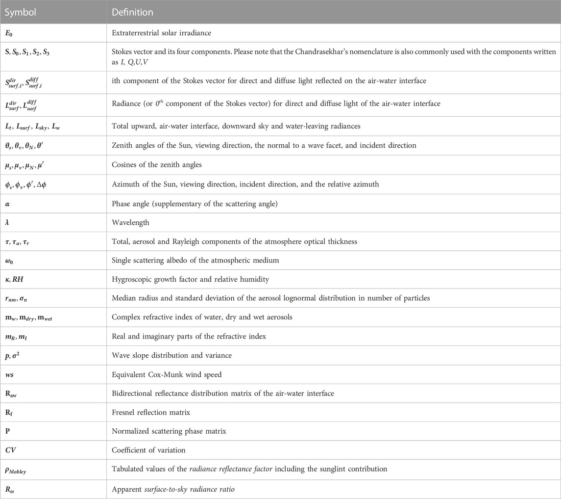
TABLE 1. Glossary of symbols.

The first AWR protocols were based on the computation of the Fresnel reflection factor to practically compute the surface radiance L_surf from the sky radiance $L_{sky}$ (Mueller and Austin, 1995). In a seminal article, Mobley (1999) proposed to further this computation with radiative transfer simulations considering a wind-ruffled air-water interface and provided tabulated values for an ad hoc term, hereafter denoted as ${\rho }_{Mobley}$, to practically compute the surface radiance from the sky radiance:

$L_{surf}\left({\theta }_s,{\theta }_v,\Delta \varphi ,\lambda \right)={\rho }_{Mobley}{L}_{sky}\left({\theta }_s,\pi -{\theta }_v,\Delta \varphi ,\lambda \right).(2)$

The surface component $L_{surf}$ might be further decomposed between the direct and diffuse components, dropping the dependencies for conciseness:

$L_{surf}=L_{surf}^{diff}+L_{surf}^{dir}.(3)$

The diffuse part is related to radiation that has undergone at least one scattering event. Conversely, the direct component is defined as the part of the sunlight radiation that has undergone reflection onto the water surface but no scattering interaction within the atmosphere. This latter component was first called Kumatage (Spooner, 1822). Thereafter, denominations such as sheen, glint or sparkle were used (Hulburt, 1934) before Cox and Munk popularized the term glitter (Cox and Munk, 1954). In the 1960s, with the first satellite pictures of Applications Technology Satellites 1 and 3 (McClain and Strong, 1969) the term sunglint has been used until today. All those terms were inspired by the very dynamic nature of the sunglint “flashes” that are controlled by the rapidly propagating waves at the water surface. Based on this erratic modulation of the sunglint intensity, protocols were designed to remove the direct component of light from L_t by taking the minimum values over a sequential series of acquisitions (Hooker et al., 2002; Zibordi et al., 2019). Moreover, recent studies investigated and proposed correction schemes for the sunglint component of the measured signal L_t (Groetsch et al., 2017; Goyens and Ruddick, 2023).

Based on those considerations, it is advocated in this study to separate the diffuse and the direct contributions to further the performances of the AWR correction schemes as already advocated in previous studies (Harmel, Gilerson, Hlaing, et al., 2012; Zhang et al., 2017). On the other hand, several names might be found in the literature for ${\rho }_{Mobley}$ such as sea surface reflectance factor (Mobley, 1999), radiance reflectance factor (Mobley, 2015), effective Fresnel reflectance coefficient (Ruddick et al., 2019). It is also worth noting that ${\rho }_{Mobley}$ is not defined as a proper reflectance but simply a ratio of two radiances with specific viewing geometries. The use of the Greek letter $\rho$, often used to define reflectance variables, might be misleading. As detailed in the next section, the direct component (i.e., sunglint) was included in Mobley’s computations (Mobley, 1999; 2015). Thus, to make a distinction with the Mobley’s parameter, a simple notation is proposed standing for surface-to-sky radiance ratio, R_ss, such as:

$R_{ss}\left({\theta }_s,{\theta }_v,\Delta \varphi ,\lambda \right)=\frac{L_{surf}^{diff}\left({\theta }_s,{\theta }_v,\Delta \varphi ,\lambda \right)}{L_{sky}\left({\theta }_s,\pi -{\theta }_v,\Delta \varphi ,\lambda \right)}.(4)$

2.1.2 Polarized nature of light

The electromagnetic radiation of light may be fully defined using the Stokes formalism. According to this formalism, four independent terms are grouped within the so-called Stokes vector that can be written using successively the indicial, Stokes (Stokes, 1852), Perrin (Perrin, 1942), and Chandrasekhar (Chandrasekhar, 1947; Chandrasekhar, 1960) nomenclatures:

$\mathbf{S}=\left(\begin{array}{l}{S}_0\\ S_1\\ S_2\\ S_3\end{array}\right)\equiv \left(\begin{array}{l}A\\ B\\ C\\ D\end{array}\right)\equiv \left(\begin{array}{l}I\\ M\\ C\\ S\end{array}\right)\equiv \left(\begin{array}{l}I\\ Q\\ U\\ V\end{array}\right).(5)$

Here, the indicial notation is preferred to get more compact equations. Using radiance unit, the term $S_0$ is equivalent to the radiance L as defined previously. The terms $S_1$ and $S_2$ describe the linear polarization and $S_3$ the circular polarization. $S_1$ quantifies the linear polarization along the vertical and horizontal planes, and $S_2$ along the+/−45° planes. It is useful to express the radiance and the other Stokes terms after substitution of the zenith angle by its cosine, $\mu =\cos \theta$. Thanks to this formalism, the radiative transfer equation can be written for an idealized plane-parallel atmosphere as follows:

$\mu \frac{d\mathbf{S}\left(\tau ,\mu ,\varphi \right)}{d\tau }=-\mathbf{S}\left(\tau ,\mu ,\varphi \right)+\frac{{\omega }_0\left(\tau \right)}{4\pi }{\displaystyle \underset{0}{\overset{2\pi }{\int }}}d{\varphi }^{\prime }{\displaystyle \underset{-1}{\overset{1}{\int }}}d{\mu }^{\prime }\mathbf{P}\left(\tau ,\mu ,\varphi ,{\mu }^{\prime },{\varphi }^{\prime }\right)\mathbf{S}\left(\tau ,{\mu }^{\prime },{\varphi }^{\prime }\right),(6)$

with $\tau$ the total (absorption + scattering) optical thickness, ${\omega }_0$ the single scattering albedo, and $\mathbf{P}$ the normalized phase matrix. The reader is referred to (Zhai et al., 2010) and references therein for the complete equations including a coupled atmosphere-water system with a rough air-water interface. This equation must be fully resolved to compute the water, surface and atmosphere (sky) radiation distributions. But, by analogy with the radiative transfer equation, the Stokes vector of the water surface can be retrieved as follows if the sky radiation distribution is known (or measured):

${\mathbf{S}}_{\mathbf{\text{surf}}}\left({\mu }_v,{\varphi }_v\right)={\mu }_s{\mathbf{R}}_{\mathbf{\text{aw}}}\left({\mu }_s,{\varphi }_s;{\mu }_v,{\varphi }_v\right)E_0{e}^{-\tau /{\mu }_s}+\frac{1}{\pi }{\displaystyle \underset{0}{\overset{2\pi }{\int }}}d{\varphi }^{\prime }{\displaystyle \underset{0}{\overset{1}{\int }}}d{\mu }^{\prime }{\mu }^{\prime }{\mathbf{R}}_{\mathbf{\text{aw}}}\left({\mu }^{\prime },{\varphi }^{\prime };{\mu }_v,{\varphi }_v\right){\mathbf{S}}_{\mathbf{\text{sky}}}\left(-{\mu }^{\prime },{\varphi }^{\prime }\right),(7)$

with E₀ the extraterrestrial solar irradiance. Note that in this formalism, the minus sign before µ indicates downward direction. In Eq. 7, the ${\mathbf{R}}_{\mathbf{\text{aw}}}$ matrix stands for the bidirectional reflectance distribution (BRD) matrix of the air-water interface projected in the reference plane (i.e., meridian plane, see Eqs 7 and 8 in (Harmel et al., 2012)). The first term of the right hand side of Eq. 7 corresponds to the direct “sunglint” contribution. Therefore, the Stokes terms can also be expressed as direct and diffuse component with:

$S_{surf,i}^{dir}\left({\mu }_v,{\varphi }_v\right)={\mu }_s{R}_{i0}^{aw}\left({\mu }_s,{\varphi }_s;{\mu }_v,{\varphi }_v\right)E_0{\text{e}}^{-\tau /{\mu }_{\text{s}}},(8)$

$S_{surf,i}^{diff}\left({\mu }_v,{\varphi }_v\right)=\frac{1}{\pi }{\displaystyle \sum _{j=0}^3}{\displaystyle \underset{0}{\overset{2\pi }{\int }}}d{\varphi }^{\prime }{\displaystyle \underset{0}{\overset{1}{\int }}}d{\mu }^{\prime }{\mu }^{\prime }{R}_{ij}^{aw}\left({\mu }^{\prime },{\varphi }^{\prime };{\mu }_v,{\varphi }_v\right)S_i^{sky}\left(-{\mu }^{\prime },{\varphi }^{\prime }\right).(9)$

Based on those equation, the surface-to-sky radiance ratio, $R_{ss}$, can be rewritten as follows where it is obvious to see that full knowledge of skylight directional distribution and its state of polarization in each celestial direction is needed:

$R_{ss}=\frac{L_{surf}}{L_{sky}}=\frac{{\displaystyle \sum _{j=0}^3}{\displaystyle \underset{0}{\overset{2\pi }{\int }}}d{\varphi }^{\prime }{\displaystyle \underset{0}{\overset{1}{\int }}}d{\mu }^{\prime }{\mu }^{\prime }{R}_{0j}^{aw}\left({\mu }^{\prime },{\varphi }^{\prime };{\mu }_v,{\varphi }_v\right)S_0^{sky}\left(-{\mu }^{\prime },{\varphi }^{\prime }\right)}{\pi S_0^{sky}\left(-{\mu }_v,{\varphi }_v\right)}.(10)$

In Mobley’s calculations (Mobley, 1999; Mobley, 2015), there is no distinction between diffuse and direct light within the Monte-Carlo resolution of the radiative transfer equation done for a pure Rayleigh atmosphere (i.e., no aerosols included). It is easy to show, in this case, that the direct sunglint component contributes to the spectral dependency of ${\rho }_{Mobley}$ through the atmosphere optical thickness parameter, $\tau \left(\lambda \right)$, that is highly spectrally variable:

${\rho }_{Mobley}=\frac{L_{surf}^{diff}\left({\mu }_v,{\varphi }_v\right)+{\mu }_s{R}_{00}^{aw}\left({\mu }_s,{\varphi }_s;{\mu }_v,{\varphi }_v\right)E_0{e}^{-\tau \left(\lambda \right)/{\mu }_s}}{L_{sky}\left(-{\mu }_v,{\varphi }_v\right)}.(11)$

2.1.3 Air-water interface

As seen in Eq. 7, the Stokes vector of the air-water interface stems from the coupling between the sky geometrical distribution of ${\mathbf{S}}_{\mathbf{\text{sky}}}$ and the BRD matrix ${\mathbf{R}}_{\mathbf{\text{aw}}}$. In the present study, this term is calculated based on the Cox-Munk isotropic wave slope distribution (Cox and Munk, 1956; Munk, 2009). Assuming that the air-water interface can be modeled as a distribution of planar wave facets defined by their orientation ${\mu }_N$ (cosine of ${\theta }_N$, see Figure 1):

${\mu }_N=\frac{{\mu }_v+{\mu }^{\prime }}{\sqrt{2\left(1+\cos \alpha \right)}},(12)$

with $\alpha$ the phase angle between incident and viewing direction:

$\cos \alpha ={\mu }_v{\mu }^{\prime }-\sqrt{1-{\mu }_v^2}\sqrt{1-{{\mu }^{\prime }}^2}\cos \Delta {\varphi }^{\prime }.(13)$

The BRD matrix can be written as:

${\mathbf{R}}_{\mathbf{\text{aw}}}\left({\mu }^{\prime },{\varphi }^{\prime };{\mu }_v,{\varphi }_v\right)=\frac{\pi {\mathbf{R}}_{\mathbf{f}}\left({\mu }_N,{\mathrm{m}}_w\right)}{4{\mu }_v{\mu }_N^4}p\left({\mu }_N,\sigma \right),(14)$

where ${\mathbf{R}}_{\mathbf{f}}$ is the Fresnel reflection matrix projected in the reference (meridian) plane, $p\left({\mu }_N,\sigma \right)$ is the statistical proportion of waves having the ${\mu }_N$ orientation, σ is the standard deviation of the wave slope distribution. It is worth highlighting that ${\mathbf{R}}_{\mathbf{f}}$ directly depends on the water refractive index, ${\mathrm{m}}_w$, in a non-linear fashion that may induce significant spectral variation of the matrix over the visible to near-infrared part of the spectrum (Harmel et al., 2018). Using the isotropic Cox-Munk model, wave slope statistics can be expressed as:

$p\left({\mu }_N,\sigma \right)=\frac{1}{\pi {\sigma }^2}\exp \left(-\frac{{\tan }^2{\theta }_N}{{\sigma }^2}\right).(15)$

For practical comparison with other studies, the variance of the slope distribution is also given in wind speed unit through the Cox-Munk parameterization, hereafter denoted as equivalent Cox-Munk wind speed:

$ws=195.3{\sigma }^2-0.586\left(\text{in }\mathrm{m}\cdot {\mathrm{s}}^{-1}\right).(16)$

2.2 Aerosol models

The aerosols in the atmosphere strongly impact the sky radiance distribution and polarization. To encompass the great variety of aerosol contents of the atmosphere, the radiative transfer simulations (i.e., resolution of Eq. 6) were performed based on the Optical Properties of Aerosols and Clouds (OPAC) models (Hess et al., 1998). The OPAC aerosol models were generated based on a mixture of pure components. Those components are representative of the main aerosol properties retrieved at the global scale. One advantage of those models is to consider non-spherical particles and the spectral variation of the complex refractive index ($\mathrm{m}=m_R+i{m}_I$) of different components of the aerosol pool. Note that the convention of positive imaginary part $m_I$ is used. The optical properties of each component are computed based on a log-normal size distribution of the number concentration of particles, N:

$\frac{dN\left(r\right)}{dr}=\frac{N_0}{{\sigma }_{n}r\sqrt{2\pi }}\exp \left(-\frac{{\left(\log \left(r/r_{nm}\right)\right)}^2}{2{\sigma }_n^2}\right),(17)$

where $r$ is the equivalent spherical radius, r_nm is the median radius of the distribution, and ${\sigma }_n$ its standard deviation. N₀ is the total number of particle per unit of volume, here taken as unity for normalization purposes; in the radiative transfer calculations this number is set via the aerosol optical thickness. For each component, the median radius is further modulated by its hygroscopic particle growth parameter, $\kappa$, (Zieger et al., 2013):

$r_{nm}=r_{dry}{\left(1+\kappa \frac{RH}{1-RH}\right)}^{1/3},(18)$

with RH the relative humidity of the atmosphere. Following the same rule of hygroscopic growth, the complex refractive index of the wet aerosols is given by:

${\mathrm{m}}_{wet}=\frac{{\mathrm{m}}_{dry}+\left(\kappa \frac{RH}{1-RH}\right){\mathrm{m}}_w}{\left(1+\kappa \frac{RH}{1-RH}\right)},(19)$

where ${\mathrm{m}}_w$ is the complex refractive index of pure water taken from Segelstein (1981). The microphysical parameters of the OPAC components used are summarized in Table 2.

TABLE 2

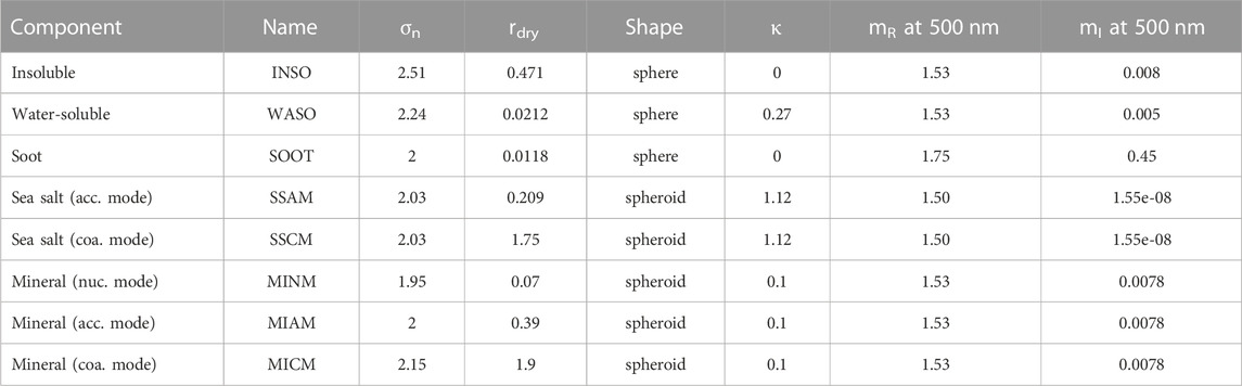
TABLE 2. Description of the microphysical parameters of the OPAC components for aerosol modeling. The refractive index values are given for the dry part. The abbreviations acc., coa. and nuc. stand for accumulation, coarse and nucleation, respectively.

The aerosol components listed above are representative of a single “species” whereas in natural conditions aerosols consist of a mixture of those components. The OPAC model provides typical mixtures of those components that are given in Table 3 for the models used in this study. The following codes were used to generate the scattering matrix with Mie theory for homogeneous sphere (Mishchenko et al., 2000), T-matrix for ellipsoidal/spheroidal particles (Mishchenko et al., 2004), those computations were extended for large particle sizes with the “Improved Geometric Optics Method” (Yang et al., 2007). The computations were performed through the MOPSMAP package (Modeled optical properties of ensembles of aerosol particles) coded in FORTRAN and based on pre-computed look-up tables (Gasteiger and Wiegner, 2018).

TABLE 3

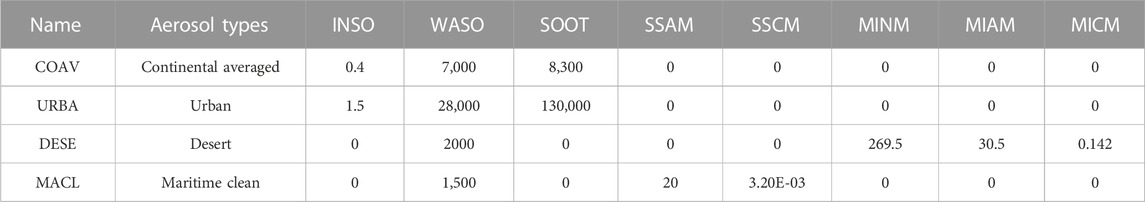
TABLE 3. Mixture of aerosol components used to generate the aerosol models.

2.3 Radiative transfer computation

The diffuse component of the Stokes vectors of the air-water interface, ${\mathbf{S}}_{\mathbf{\text{surf}}}$, and sky, ${\mathbf{S}}_{\mathbf{\text{sky}}}$, were computed at the bottom of the atmosphere level using the Ordres Successifs Océan Atmosphère Avancé (OSOAA) code (Chami et al., 2015). This code is based on the successive order method developed for atmosphere application (Deuze et al., 1989; Lenoble et al., 2007) with addition of the coupling with a water layer (Chami et al., 2001). Here, the water layer was set as totally absorbing to compute the contribution of the air-water interface, i.e., the water-leaving radiance is null. Sky and direct sunlight reflections on the water surface are taken into account to solve the radiative transfer Equation 6 but the sunglint contribution to the surface radiation was removed afterward. Angular integrations were based on sixty Gaussian nodes and the maximum order of Fourier expansion in azimuth was set to 1,024 for the scattering matrices and 2048 for the air-water interface BRD matrix. No truncation was applied to the scattering phase functions.

The computations were repeated for a comprehensive series of input parameters which are listed in Table 4. The atmosphere is modeled as a mixture of non-absorbing molecules (i.e., Rayleigh scattering) and aerosols. The Rayleigh optical thickness, ${\tau }_r$, decreases exponentially with the altitude with the scale height of 8 km, similarly a scale height of 2 km was set for the aerosol optical thickness. The spectral values of ${\tau }_r$ and the depolarization factor were taken from (Bodhaine et al., 1999). As to the aerosol optical properties, the four OPAC models listed in Table 3 were used to implement the scattering matrices and the absorption and extinction cross sections. To limit the number of aerosol models the relative humidity was set to 70%. The BRD matrix of the air-water interface, ${\mathbf{R}}_{\mathbf{\text{aw}}}$, was modeled following Eq. 14 with the spectral values of the water refractive index computing as in (Harmel et al., 2018) based on tabulated values (Quan and Fry, 1995; Max and Chapados, 2009; Kedenburg et al., 2012).

TABLE 4

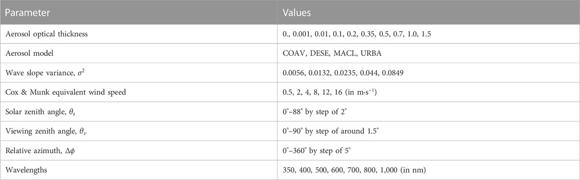
TABLE 4. Summary of the input parameters used to generate the look-up tables (LUT).

2.4 Uncertainty calculus

The surface-to-sky radiance ratios, $R_{ss}$, were computed by fixing the aerosol and water surface BRD matrix parameters. In practice, those parameters are in the best case scenario known with a given uncertainty or totally unknown if no associated measurements are performed concurrently. In the proposed model, the input parameters, noted $x_i$ below, are the aerosol optical thickness at 550 nm, the aerosol model and the wind speed, or reciprocally the variance of the wave slope distribution. In order to document the impact of unknown or partially known input parameters two different metrics are used. The first one is the coefficient of variation, CV, computed as follows:

$CV=\frac{\sqrt{\frac{1}{N_x}{{\displaystyle \sum _i^{N_x}}\left(R_{ss}\left(x_i\right)-\overline{R_{ss}}\right)}^2}}{\overline{R_{ss}}},(20)$

where N_x is the number of input parameters and $\overline{R_{ss}}$ the average computed over the N_x parameters considered. The second metric is the standard deviation of $R_{ss}$ due to the propagation of errors made in the input parameters. This can be understood as the uncertainty attached to the surface-to-sky radiance ratio assuming uncorrelated Gaussian errors in aerosol optical thickness, ${\tau }_a$, and wave slope distribution (Eq. 15) set through the wind speed parameter, ws:

$\Delta R_{ss}=\sqrt{{\left(\frac{\partial R_{ss}}{\partial {\tau }_a}\right)}^2\Delta {{\tau }_a}^2+{\left(\frac{\partial R_{ss}}{\partial ws}\right)}^2\Delta w{s}^2.}(21)$

Following uncertainty estimation based on large scale comparisons (Harmel and Chami, 2012; Levy et al., 2013), the errors were modeled as linear function as follows:

$\left\{\begin{array}{l}\Delta {\tau }_a=0.2{\tau }_a+0.05\\ \Delta ws=0.2ws+0.5\left(\text{in }m\cdot s^{-1}\right)\end{array}\right..(22)$

3 Results

3.1 Rayleigh atmosphere

The surface-to-sky radiance ratio is first shown for a pure Rayleigh atmosphere (i.e., no aerosol). To illustrate the computation the downward (celestial) and upward (surface) radiance distribution are plotted in Figure 2 given in normalized radiance unit (i.e., actual radiance multiplied by $\pi /E_0$). As already mentioned, the direct light component was removed to analyze the diffuse component only. This is why no strong peak is seen for null relative azimuth around the solar zenith angle. For this pure molecular condition, the spectral variation of the sky and surface radiance distribution is very weak. But, a spectral behavior is clearly visible within the $R_{ss}$ angular distribution (see bottom row in Figure 2). In this configuration, the minimum skylight reflection occurs for relative azimuth of 90° (symmetrically 270°) and viewing zenith angles between 30° and 40°. Interestingly, those minima occur in the typical angular region of the neutral points where the degree polarization of the reflected light is null (Fraser, 1968; Adams and Kattawar, 1997). Conversely, the highest reflections appear for relative azimuths close to 180°, that is to say when the Sun is behind the observing system. It is also interesting to note that the value of $R_{ss}$ increases with diminishing wavelengths where the molecular atmosphere is the most scattering, in other terms, when the diffuse light proportion increases.

FIGURE 2

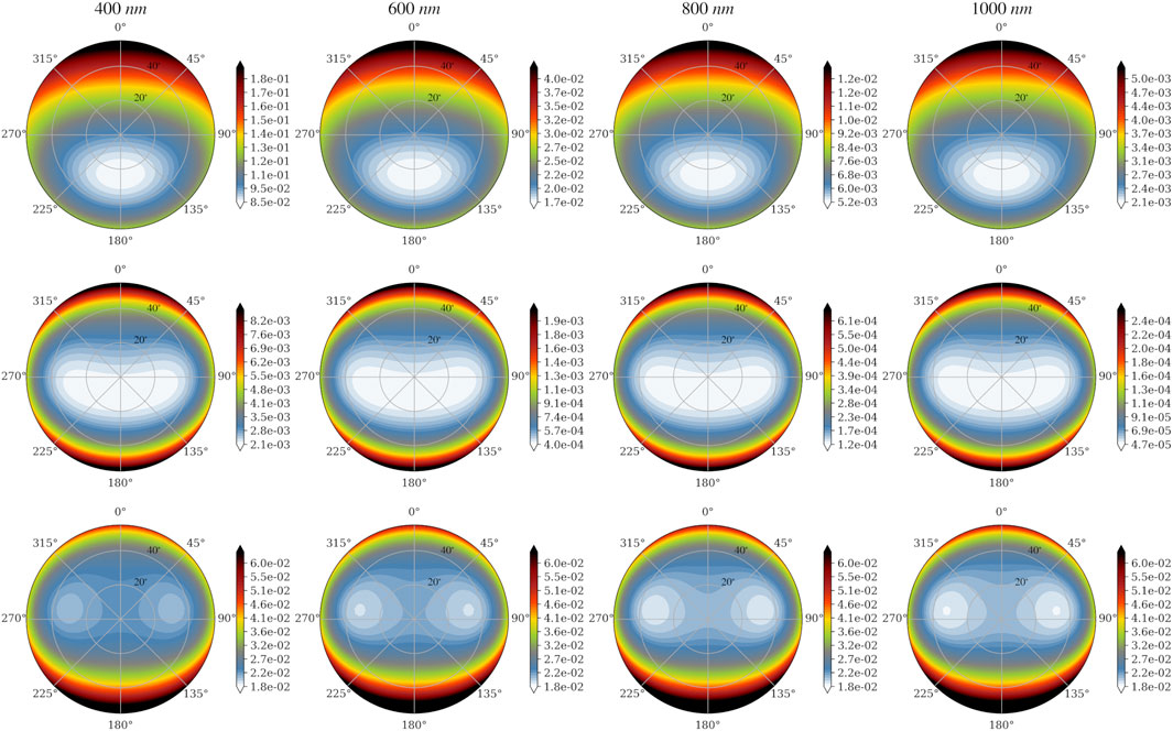
FIGURE 2. Polar view of the downward sky radiance $L_{sky}^{diff}$ (first row), upward surface reflected radiance $L_{surf}^{diff}$ (second row), and the resulting surface-to-sky radiance ratio (bottom row) for a solar zenith angle ${\theta }_s$ = 50°, and a wave slope variance ${\sigma }^2$ = 0.0132 (i.e., Cox-Munk wind speed of 2 m s⁻¹). Each column corresponds to the indicated wavelength. Note that the concentric circles correspond to the viewing zenith angles of 20° and 40° and radial angles represent the relative azimuth to the Sun. By convention, the relative azimuth is equal to 0° when the Sun and the sensor are in opposition.

Beside this spectral dependence, $R_{ss}$ values are mainly driven by the viewing observation and the state of the wavy water surface. Figure 3 shows the $R_{ss}$ values at a fixed wavelength 600 nm for various solar viewing angles and wave slope distributions. The potential impact of the sunglint contribution is also displayed in this figure. Obviously, the angular distribution of $R_{ss}$ is not significantly disturbed within the sunglint area since only diffuse light is considered. For lower wind speed conditions, the minimum values of skylight reflection are outside the sunglint area which is not the case for higher wind speeds or when the Sun is close to zenith. It is also important to note that when the Sun is lower on the horizon, the $R_{ss}$ values are rapidly changing with azimuth that should be accurately known in this case.

FIGURE 3

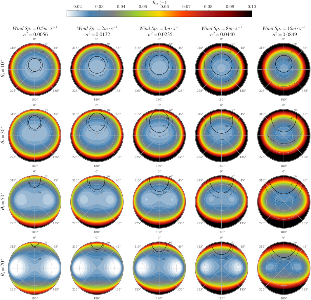
FIGURE 3. Polar diagrams of the surface-to-sky radiance ratios, $R_{ss}$, at 600 nm for a pure Rayleigh atmosphere and several configurations: each row corresponds to a given solar zenith angle (from 10° to 70°), each column corresponds to a given wave slope distribution expressed through its variance or the equivalent Cox-Munk wind speed. For information, contour lines for sunglint reflectance of 1% (dotted black line) and 5% (continuous line) are superimposed based on the Cox-Munk isotropic model.

Another view of the $R_{ss}$ sensitivity in a Rayleigh atmosphere is given Figure 4 where the ratio calculated at 500 nm is extracted for a relative azimuth of 90° and 135° for a viewing zenith angle of 40°. In this way, the computed values can be compared with previous tabulated calculations performed without polarization (Mobley, 1999) and with polarization for a Rayleigh atmosphere (Mobley, 2015). First, it is readily observable that Mobley’s ratios increase sharply with the decreasing solar zenith angle where the direct light from sunglint becomes more pronounced. The corresponding $R_{ss}$ values from this study are displayed with and without considering the sunglint component in the calculations (last column of Figure 4). Clearly, the consideration of sunglint within the ratio calculation produces a significant increase of its value toward low solar zenith angles; the sunglint signal rapidly overwhelms the reflected-skylight signal with increasing wind speeds. For instance, at solar zenith angle 10° and wind speed 12 m s⁻¹, actual $R_{ss}$ computed for diffuse light is around 0.045 and addition of sunglint increases the value up to 0.065 for ${\theta }_v$ = 40° and $\Delta \varphi$ = 90°. It is worth remembering that the sunglint signal is strongly wavelength dependent through the action of the direct transmittance of the atmosphere (see Eq. 8). Unspectral consideration of sunglint yields extremely high $R_{ss}$ values for molecular atmosphere which can partly explain the overcorrection and enhanced uncertainty at small solar zenith angles (Harmel et al., 2011), overcorrection is only suppressed when only diffuse light is considered as shown in the Figure 7 of (Harmel et al., 2012). It is shown here that the contribution of sunglint is still significant for solar angles up to 40° where continuous and dashed curves depart from each other in the last column of Figure 4. Notwithstanding the sunglint impact, it is important to highlight that the two calculations including polarization provide quite similar values and shape with varying solar zenith angles (see M2015 and this study in Figure 4) when compared to the unpolarized calculation (M1999).

FIGURE 4

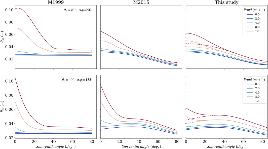
FIGURE 4. Tabulated values of the surface-to-sky ratio computed (first column) without consideration of polarization (Mobley, 1999), (second column) accounting for polarization within a Rayleigh atmosphere (Mobley, 2015) and (third column) this study for pure diffuse light (dashed curves) and with addition of the sunglint component (solid curves). Geometry and equivalent Cox-Munk wind speed are indicated in the insets.

The spectral values of $R_{ss}$ are shown in Figure 5 for a Rayleigh atmosphere for three different viewing zenith angles and two relative azimuths commonly used for AWR acquisitions. These values exhibit conspicuous spectral dependencies with diverse amplitudes depending on both the viewing geometry and the water surface roughness here considered through the equivalent Cox-Munk wind speeds. In general, the ratios decrease with the wavelength for low wind speed conditions up to 4 m s⁻¹. Exceptions might occur for the viewing zenith angle 50° when the Sun is high on the horizon. In all cases, increase in wind speed produces an overall increase of the $R_{ss}$ values with more marked spectral dependencies. In parallel, such modifications of the wave slope variance induce spectral increase of the values toward the near-infrared part of the spectrum. This spectral feature is more pronounced when using 135° for the relative azimuth. As a result of the surface roughness effect, the dependency on wind speed is smaller toward the shorter wavelengths.

FIGURE 5

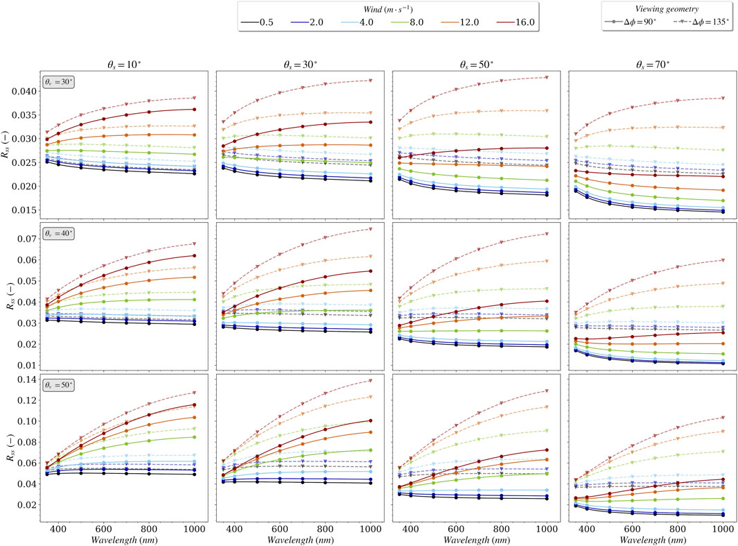
FIGURE 5. Spectral values of the surface-to-sky radiance factor, $R_{ss}$, for a Rayleigh atmosphere given for three viewing zenith angles of 30°, 40° and 50° (rows) and two relative azimuths of 90° (continuous lines), and 135° (dashed lines).

3.2 Impact of aerosols

3.2.1 Spectral considerations

The presence of aerosols in the atmosphere modifies the downward radiance distribution but also the state of polarization of the celestial hemisphere. The impact of aerosols on the spectral values of $R_{ss}$ is analyzed in this section. The Figures 6, 7 show the spectral dependency of $R_{ss}$ under atmosphere with various loads in maritime clean (MACL) aerosols for a viewing angle of 40° and relative azimuths of 90° and 135°, respectively. Similar results obtained for the aerosol models COAV, DESE and URBA are provided in the Supplementary Material. In all the configurations shown, the addition of aerosols in the atmosphere induces a significant modification of the $R_{ss}$ values from the Rayleigh case. It is notable that the departure from the Rayleigh-case values starts for aerosol optical thickness as low as 0.01. In general, the aerosol optical thickness is around 0.1 for clear atmospheres, around 0.4 for moderately turbid and can reach values greater than 1.5 for extremely turbid atmospheres. From the results shown here no specific behavior on $R_{ss}$ can be attributed to changes in the aerosol load: for relative azimuth 90° and according to the sun’s zenith angle and surface state the values might be either decreased or increased by addition of aerosol within the atmosphere. As to relative azimuth 135°, increase in aerosol load always produces decrease of the $R_{ss}$ spectral values. Nevertheless, it should be pointed out that the values provided by the polarized values M2015 tabulated (Mobley et al., 2015) are always closer than the unpolarized version M1999 (Mobley, 1999) to the computed $R_{ss}$ for low aerosol optical thickness and in particular for the Rayleigh atmosphere. Intersections are even observed between M2015 and the computed spectral values around 550 nm at which M2015 values were computed for a Rayleigh atmosphere. This demonstrates the consistency between the two computations but, in turn, highlights the need to consider the aerosol component for surface light correction in AWR protocols.

FIGURE 6

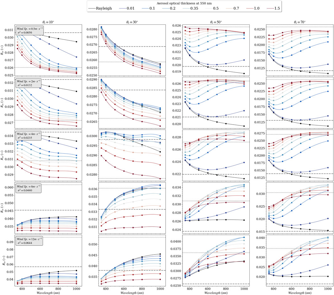
FIGURE 6. Spectral values the surface-to-sky radiance factor, $R_{ss}$, for several aerosol loads within the atmosphere considering the maritime clean (MACL) aerosol model for viewing zenith angle 40° and relative azimuth 90°. Values are shown for several solar zenith angles (columns) and wave slope variance (rows). The unspectral values from previous studies are also displayed with gray lines for M1999 (Mobley, 1999) (dotted lines) and M2015 (Mobley, 2015) (dashed lines).

FIGURE 7

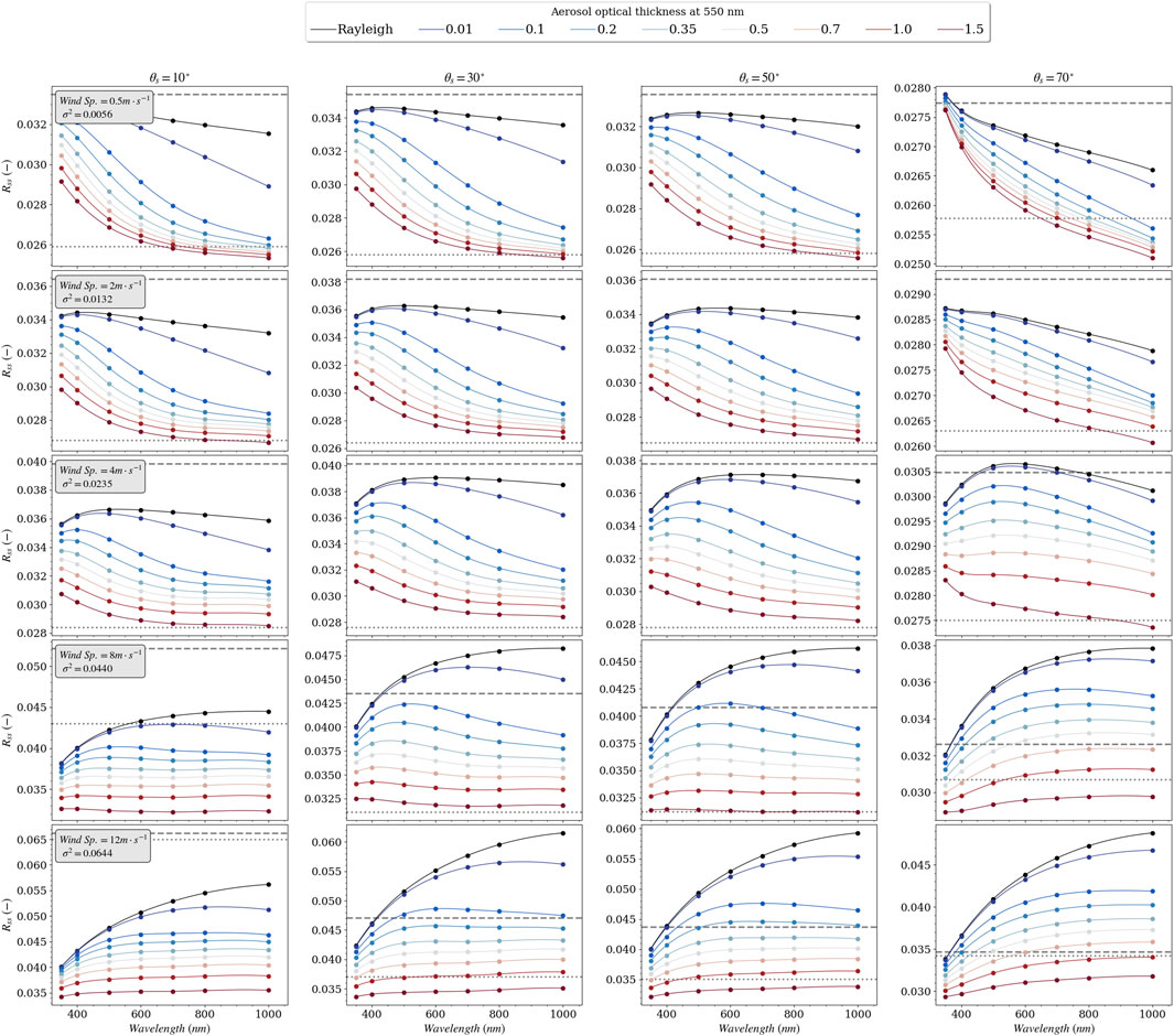
FIGURE 7. Similar to Figure 6 for relative azimuth 135°.

3.2.2 Directional considerations

In order to examine the sensitivity of $R_{ss}$ to the viewing geometry, it is of interest to analyze the polar diagrams displayed in Figure 8 for various solar zenith angles and the four aerosol models corresponding to maritime (MACL) or continental (COAV) environments, polluted areas (URBA) and desert dust impacted atmospheres (DESE). Those aerosol models differ between each other by their respective scattering matrix and absorption properties. The models MACL and DESE correspond to coarse size aerosols with a highly peaked scattering function in forward scattering angles. Conversely, COAV and URBA represent smaller particles exhibiting a smoother forward peak of the scattering phase function and more pronounced side and backward scattering. As a result, it is clearly seen from Figure 8 that MACL and DESE induce a narrow pattern of low $R_{ss}$ in the sunglint area (white spots in the figure). This pattern is diminished and more spread in the case of finer aerosols (COAV and URBA). In addition to this geometrical pattern, changes due to the aerosol model can be noticed for other viewing angles and azimuths. This reinforces the need to consider the aerosol load of the atmosphere both with the optical thickness but also the aerosol models defined by their inherent microphysical properties (or optical properties).

FIGURE 8

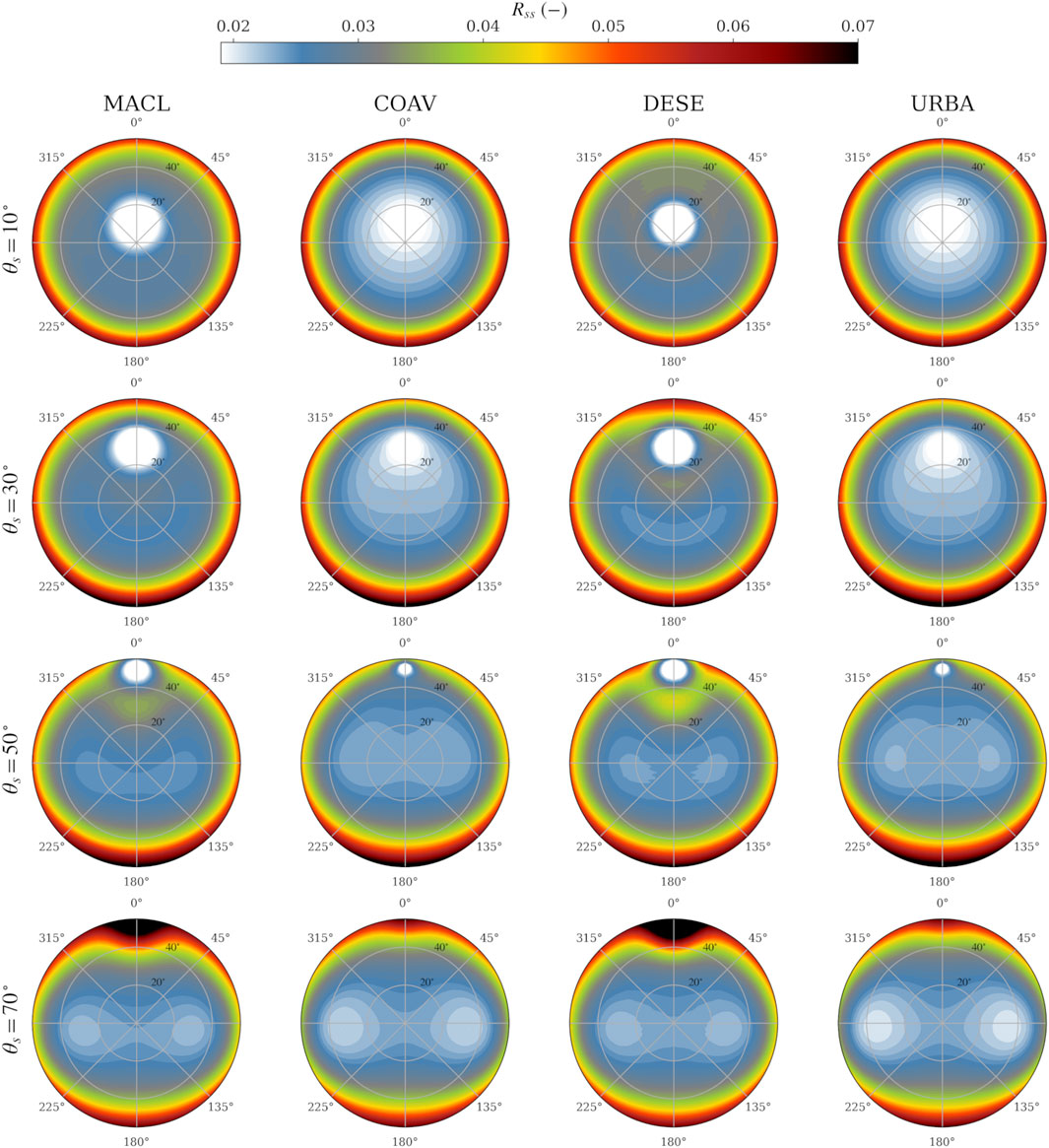
FIGURE 8. Polar diagrams of $R_{ss}$ calculated at 600 nm for several solar zenith angles (rows) and four aerosol models: maritime clean (MACL), continental average (COAV), desert dust (DESE) and polluted urban (URBA). Values are given for an aerosol optical thickness of 0.35 and equivalent Cox-Munk wind speed of 4 m s⁻¹ (i.e., ${\sigma }^2$ = 0.0235).

Most of the protocols advise to use a viewing zenith angle of 40°. On the other hand, for fixed platforms the sensor can either be rotated to get a constant relative azimuth with respect to the Sun or just left immobile making the relative azimuth change over the course of a day (Harmel et al., 2011). In order to examine the impacts of varying solar and azimuth angles, it is practical to replot the polar diagrams for all the solar zenith angles by fixing the viewing angle. Figure 9 shows this kind of polar diagram for the MACL conditions and several water surface states. Similar figures are provided in the Supplementary Material for the other aerosol models. From this figure, it can be noted that the lowest $R_{ss}$, i.e., minimizing the sky reflection effect, occur for relative azimuths centered around 90°. In comparison, $R_{ss}$ exhibits higher values along relative azimuth 135°, that is to say the impact of skylight reflection is more pronounced for this viewing geometry. On the other hand, it should be noted that values for relative azimuths between roughly 120° and 250° are significantly increased in high wind speed conditions. In any case, the exact viewing configuration should be accurately known to obtain the corresponding surface-to-sky radiance ratio for practical correction within the AWR processing scheme.

FIGURE 9

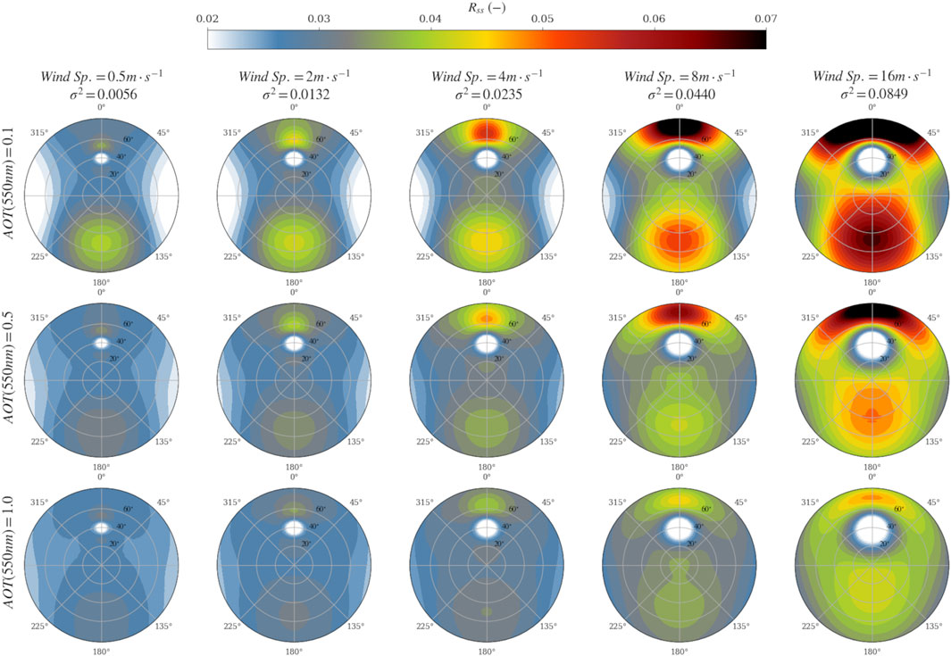
FIGURE 9. (polar diagram: contour circles indicate solar zenith angles) Directional values of $R_{ss}$ at 600 nm for a fixed viewing zenith angle of 40° and various loads in maritime clean (MACL) aerosols (rows) and water surface states (columns).

3.3 Uncertainties

3.3.1 Aerosol models

As shown in the previous figures, the aerosol optical thickness and the aerosol model produce significant modifications of the skylight reflected by the air-water interface toward the AWR sensor. In practice, it is far from being obvious to exactly know the exact optical properties of the aerosol load in presence. The directional variability of $R_{ss}$ was shown in Figure 9 for a given aerosol model mimicking typical salt aerosols retrieved in the maritime environment. It is of interest to quantify the variation of this term due to unknown aerosol models. For this purpose, the coefficient of variation (CV) due to unknown aerosol models was computed over the four aerosol models based on Eq. 20. The resulting CV are shown in Figure 10 for several atmosphere turbidites and water surface states. The variations are obviously minimal for low aerosol optical thickness but can reach a few percent for high solar zenith angle, in particular at the relative azimuth of 90°. In comparison, CV is smaller when using a relative azimuth of 135° for measurements with values below 2%. On the contrary, CV values significantly increase for relative azimuths of 180° or smaller than 90°. Choosing an appropriate relative azimuth for a given solar zenith angle might help minimize uncertainty in the surface radiance correction even if the aerosol type is unknown.

FIGURE 10

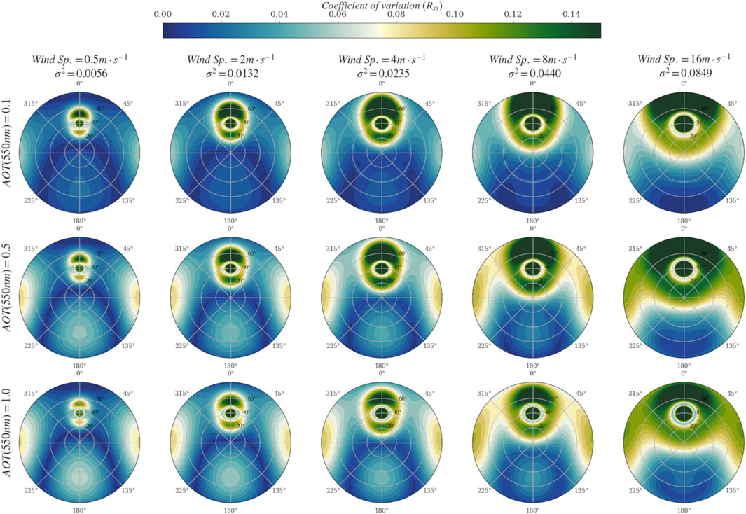
FIGURE 10. (polar diagram: contour circles indicate solar zenith angles) Coefficient of variation due to unknown aerosol model computed from the following OPAC models: Maritime clean, Continental average, Desert dust, Urban for a relative humidity of 70%. Values computed at 600 nm for a viewing angle of 40° for diverse (columns) wind speeds (or wave slope variances, σ²) and (rows) aerosol optical thicknesses.

3.3.2 Propagation of errors from aerosol optical thickness and wind speed

The uncertainties of the surface-to-sky radiance ratio were computed based on Eqs 21 and 22 to account for the propagation of the errors attached to the input parameters. The two numerical parameters ${\tau }_a$ and $ws$ were taken into account enabling proper analytical derivation in the calculation. The absolute uncertainty was then divided by corresponding $R_{ss}$ to obtain the relative uncertainty as shown in Figure 11 for wavelength 600 nm. Similar figures for wavelengths 350 and 1,000 nm are provided in the Supplementary Material. From those figures, it is clearly seen that the uncertainty is very variable from one given observing geometry to another with values starting from tens of percent up to over 15%. Interestingly, the uncertainties decrease with the atmosphere turbidity set through the aerosol optical thickness, ${\tau }_a$. This can be explained by two different effects: (i) the relative error in ${\tau }_a$ decreases with increasing aerosol load, (ii) the skylight distribution gets more isotropic under turbid atmosphere conditions. The first effect comes from the error model used for ${\tau }_a$ in which it is assumed that the relative error diminishes with increasing ${\tau }_a$; this assumption is due to the fact that actual measurements of the optical thickness are more precise for greater values of ${\tau }_a$ (Knobelspiesse et al., 2004). For instance, based on Eq. 22, relative error is 0.7 for ${\tau }_a$ = 0.1 and 0.25 for ${\tau }_a$ = 1.0. The second effect is more physical. When the aerosol optical thickness increases, more multiple scattering occurs in the atmosphere inducing a more isotropic distribution of the sky radiance. As a result, the skylight reflection on the waves at the water surface is less sensitive to the orientation of their facets. Therefore, errors in the wave slope distribution produce a lesser impact on $R_{ss}$ computed for such conditions.

FIGURE 11

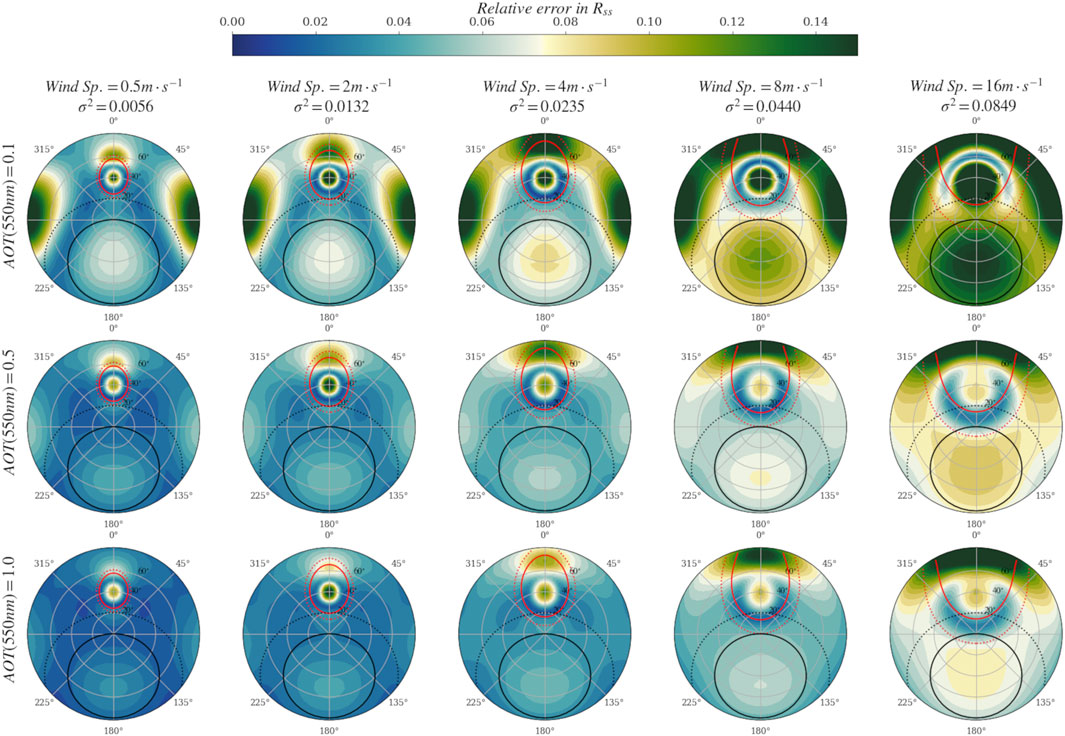
FIGURE 11. (polar diagram: contour circles indicate solar zenith angles) Relative uncertainty in $R_{ss}$ at 600 nm and ${\theta }_v$ = 40° due to propagation of errors attached to input aerosol optical thickness and equivalent Cox-Munk wind speed. For information, contour lines for sunglint reflectance of 1% (dotted red line) and 5% (continuous red line) are superimposed based on the Cox-Munk isotropic model. Contour lines of scattering angle 120° (dotted black line) and 140° (continuous black line) are also indicated.

Another interesting aspect is the angular distribution of the uncertainty. Finding the viewing geometry to minimize the uncertainty might help improve the performances of the overall AWR process. For clear atmosphere conditions (i.e., ${\tau }_a$ = 0.1) and low wind speed, it can be seen in Figure 11 that the uncertainty strongly increase with solar zenith angle for relative azimuth 90°, with values exceeding 10% for ${\theta }_s$ >50°. On the contrary, the uncertainty values remain under 2% for the same conditions when taking a relative azimuth of 135°. A specific angular zone between scattering angle 120° and 140° was noticed to provide lesser uncertainty, this zone is delimited by the two black lines in Figure 11, similar patterns are also observed in the absolute uncertainty values. It is worth noting that this geometrical zone provides the lowest uncertainty values whatever the parameters ${\tau }_a$ and $ws$ considered. This provides a way to minimize AWR uncertainty by adapting the relative azimuth for each specific Sun elevation.

4 Discussion

4.1 Diffuse and direct light

In this study, it has been proposed to separate the contribution of the diffuse skylight from the direct component of the sunglint radiance to correct AWR measurements for surface reflection. This is the main difference with previously proposed values of the sky to surface radiance conversion factor provided by Mobley (1999) assuming unpolarized light and Mobley (2015) which account for polarization where the sunglint is embedded. Those values were computed for a fixed wavelength (e.g., 550 nm) assuming the factor is spectrally neutral (Mobley, 2015). It has been shown that the inclusion of the sunglint should also take into account the spectral variation of the direct atmospheric transmittance through the dependency of the total optical thickness including the aerosol effect on it. Other studies provided spectral values of this factor from unpolarized (Lin et al., 2023) or full vector (Gilerson et al., 2018) radiative transfer computations. But, both studies included the sunglint contribution to the final computation. Note that another study explicitly separated the diffuse and direct contributions recommending a two-step procedure for respective corrections of sky and sun lights (Zhang et al., 2017). It has been shown in Figure 4 that inclusion of sunglint induces significant discrepancies especially for low solar zenith angle (i.e., Sun close to zenith). On the other hand, it was already noted that the application of standard procedure that takes the quantile 20% of the measured L_t (Hooker et al., 2002) with factor including the sunglint contribution generally leads to overcorrecting the water signal in the current AERONET-OC processing with increased uncertainty for high Sun elevation (Harmel et al., 2011; Harmel et al., 2012). Moreover, the usual wave statistics fail to reproduce the sunglint signal based on surface wind speed measurements over short time scale and/or small spatial extent (Kay et al., 2009). This study provides spectral values for diffuse light correction for a comprehensive set of environmental conditions that can help to further constrain the dedicated sunglint correction step as recently proposed (Goyens and Ruddick, 2023). It can also be foreseen that preliminary diffuse light correction could help to extract the sunglint signal from spectral measurement where the water-leaving radiance is negligible (e.g., shortwave-infrared) as done for atmospheric correction of optical satellite (Harmel et al., 2018).

4.2 Surface roughness

The presented results are based on the isotropic Cox-Munk wave slopes statistics (Cox and Munk, 1954). This model was used due to its simplicity to be included in radiative transfer calculation. The surface-to-sky radiance ratio has been tabulated using the equivalent Cox-Munk wind speed but also with the variance of the wave slope distribution. This enables the use of the appropriate value based on water surface state information instead of wind speed that may be uncorrelated to actual surface roughness as already mentioned (Kay et al., 2009). Nevertheless, perspectives of this work should include advanced numerical simulations of the wave spectra (from gravities to capillaries) and their slope distributions provided by several theoretical studies based on the Monte-Carlo approach (Mobley, 2015; D’Alimonte and Kajiyama, 2016; Foster and Gilerson, 2016; Hieronymi, 2016). Another approach could be based on direct measurements of the wave distribution from polarimetric measurements (Zappa et al., 2008)) or from multi-angular upwelling radiance measurements as recently suggested (Goyens and Ruddick, 2023).

4.3 Aerosol approach

As it has been shown, the presence of aerosols significantly modifies the surface-to-sky radiance ratio through their optical thickness but also the inherent optical properties defining the aerosol model to be used. These modifications arise even for low values of the aerosol optical thickness. Even if the viewing geometry can be adapted to minimize uncertainty due to partially known aerosol properties, as shown in Figures 10, 11, it is necessary to document the presence of aerosol load during data acquisitions. This can easily be done from the measurements provided by the AERONET-OC network (Zibordi et al., 2009) for which measurements are routinely operated to provide spectral aerosol optical thickness (Zibordi et al., 2021) or further optical properties (Dubovik et al., 2000; O’Neill et al., 2003). For another important network called HYPERNETS, the installed system, the HYperspectral Pointable System for Terrestrial and Aquatic Radiometry (HYPSTAR), could also be used to concurrently monitor the aerosol optical properties but it is not currently the case for routine operation (Goyens et al., 2022). A recent study showed the benefits of incorporating a pyranometer in the AWR system enabling distinctive measurements of the direct and diffuse part of the downwelling irradiance (Jordan et al., 2022). For this kind of system, the pyranometer measurements could also be used to retrieve the aerosol parameters (Alexandrov et al., 2002).

Above-water radiometry methods are also deployed on small to big ships including research vessels (Ondrusek et al., 2022), ferries (Nasiha et al., 2022) or even dugout canoes (Marinho et al., 2021). In such conditions, the aerosol properties are not always acquired concurrently. A first approach could be to use the aerosol data provided by the operational reanalysis models such as Copernicus’ CAMS or NASA’s MERRA which provide aerosol optical properties worldwide with acceptable uncertainties (Gueymard and Yang, 2020). Another practical approach would be to systematically perform aerosol data acquisition within AWR protocols. For this purpose, hand-held sun photometers could be advantageously exploited to provide spectral aerosol optical thickness (Porter et al., 2001; Knobelspiesse et al., 2004).

4.4 Impacts of geometrical configuration

The above-water radiometry procedure is based on a well-calibrated radiometer positioned in predetermined viewing configuration by setting both the viewing zenith angle and the relative azimuth. Even if the choice of viewing geometries for real-world installation may suffer limitations due to the constraints imposed by the vessel/platform superstructure or associated shadowing, it is worth documenting the most optimal geometries that help minimize uncertainties. This study showed that the absolute value of surface-to-sky radiance ratio is very variable with these two parameters but also the uncertainty attached to $R_{ss}$. This uncertainty originates from errors made in the input parameters to the presented model, i.e., aerosol optical thickness and type as well as the surface roughness parameter. It has been demonstrated that the uncertainty can be minimized by changing the relative azimuth with respect to the Sun elevation to perform the AWR acquisition in a geometry following a constant scattering angle value centered on approximately 135° irrespective of the wavelength. Therefore, it is recommended to adapt the viewing geometry over the course of a day. To do so, the couple $\left({\theta }_s,\Delta \varphi \right)$ needs to be adapted to get a constant value of the scattering angle for a fixed viewing zenith angle, ${\theta }_v$. The Figure 12 shows this relationship between ${\theta }_s$ and $\Delta \varphi$ for ${\theta }_v$ = 40° for three values of the scattering angles where the uncertainties are minimal. From this figure, it is recommended to perform the acquisition at $\Delta \varphi$ = 90° when the Sun is at ${\theta }_s$ = 20° and at $\Delta \varphi$ = 150° when the Sun is at ${\theta }_s$ = 80°, for instance. For robotic setups, the viewing configuration could be automatically adapted from the exact Sun location following this scheme.

FIGURE 12

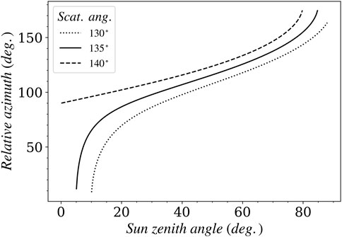
FIGURE 12. Optimal viewing geometry of above-water radiometer for a viewing zenith angle of 40° according to lowest uncertainty attached to the R_ss factor which is centered on scattering angle 135°, see Figure 11.

5 Conclusion

The impact of aerosols, polarization and water surface roughness on above-water radiometry (AWR) measurements was analyzed based on full vector radiative transfer computations. Based on theoretical and practical considerations, the parameter to convert the downward sky radiance measurements into the surface-reflected radiance was renamed surface-to-sky radiance ratio, $R_{ss}$, in order to avoid misuse of the term reflectance as often encountered in the literature. Angular values of $R_{ss}$ were computed for a large set of input parameters with surface roughness both expressed in wave slope variances (0.0056–0.0849) or equivalent Cox-Munk wind speeds (0.5–16 m s⁻¹), aerosol optical thicknesses (0–1.5 at 550 nm), aerosol types covering maritime, continental, desert and polluted conditions, and for wavelengths ranging from 350 to 1,000 nm. Here, the use of the slope variances is due to the fact that statistics between roughness and wind speed might not hold for time and space scales encountered in AWR measurements. Following previous studies, diffuse (skylight) and direct (sunglint) light component have been separated to provide $R_{ss}$ values for diffuse light only. Comparison with former tabulated values including sunglint might explain the overestimation of the surface radiance when the Sun is high on the horizon.

It has been shown that knowledge on aerosol load and type is critical to correct for reflected skylight even for very low amounts in the atmosphere. Uncertainties attached to $R_{ss}$ were computed based on the two input parameters slope variance (wind speed) and aerosol optical thickness. The uncertainty is very sensitive to the viewing direction and Sun elevation exhibiting lower values for geometries defined by a scattering angle between 120° and 140°. This enabled defining the most appropriate couple of viewing and azimuth angles to reduce uncertainty for a given Sun angle. For instance, it has been recommended to perform acquisition for viewing zenith angle 40° and relative azimuth 90° when the Sun zenith angle is 20° and relative azimuth 150° when the Sun zenith angle is 80°. Such adaptable geometries could be implemented in robotic AWR systems to reduce uncertainty budget. Even if the uncertainty due to unknown aerosol optical properties can be minimized, it is advocated to accompany AWR acquisitions with concurrent aerosol measurements to further constrain the surface-reflected light correction.

The computations presented in this study still need to be further applied on actual in situ data sets. To this end, tabulated values are provided as a multidimensional data set based on the network Common Data Form (netCDF file). It is worth highlighting that the tabulated values must be used under clear sky conditions only since heterogeneous atmospheres with clouds or fully overcast conditions were not considered. Nevertheless, those values could be used to develop optimal methods to proceed with non-ideal conditions as in (Groetsch et al., 2017; Pitarch et al., 2020; Borges et al., 2022). The correction of the sunglint component is not taken into account in the tabulated values but methods based on separation of diffuse and direct light developed for atmospheric correction could be further investigated (Harmel et al., 2018). Even if the results have been discussed for monodirectional radiometer, the tabulated values are also suitable for correction of AWR multi-view radiometric camera if the viewing geometry of each pixel is known (Carrizo et al., 2019; Gilerson et al., 2020). Finally, the theoretical scheme presented here could be easily adapted to provide spectral values to correct polarimetric measurements of the water system.

Data availability statement

The original contributions presented in the study are included in the article/supplementary material, further inquiries can be directed to the corresponding author.

Author contributions

TH: Conceptualization, Data curation, Funding acquisition, Investigation, Methodology, Software, Visualization, Writing–original draft.

Funding

The author(s) declare financial support was received for the research, authorship, and/or publication of this article. French National Program for Remote Sensing (PNTS-2019-13).

Acknowledgments

The author is thankful to Alexandre Castagna and the GEO AquaWatch Nomenclature Group for insightful discussions. The editor and the two reviewers are also gratefully acknowledged for their subtle and enriching comments.

Conflict of interest

TH was employed by Magellium Artal Group.

Publisher’s note

All claims expressed in this article are solely those of the authors and do not necessarily represent those of their affiliated organizations, or those of the publisher, the editors and the reviewers. Any product that may be evaluated in this article, or claim that may be made by its manufacturer, is not guaranteed or endorsed by the publisher.

Supplementary material

The Supplementary Material for this article can be found online at: https://www.frontiersin.org/articles/10.3389/frsen.2023.1307976/full#supplementary-material

References

Adams, J. T., and Kattawar, G. W. (1997). Neutral points in an atmosphere-ocean system. 1: upwelling light field’, Applied Optics. Opt. Soc. Am. 36 (9), 1976–1986. doi:10.1364/ao.36.001976

PubMed Abstract | CrossRef Full Text | Google Scholar

Alexandrov, M. D., Lacis, A. A., Carlson, B. E., and Cairns, B. (2002). Remote sensing of atmospheric aerosols and trace gases by means of multifilter rotating shadowband radiometer. Part II: climatological applications. J. Atmos. Sci. 59 (3), 544–566. doi:10.1175/1520-0469(2002)059<0544:rsoaaa>2.0.co;2

CrossRef Full Text | Google Scholar

Antoine, D., d'Ortenzio, F., Hooker, S. B., Bécu, G., Gentili, B., Tailliez, D., et al. (2008). Assessment of uncertainty in the ocean reflectance determined by three satellite ocean color sensors (MERIS, SeaWiFS and MODIS-A) at an offshore site in the Mediterranean Sea (BOUSSOLE project). J. Geophys. Res. Am. Geophys. Union 113 (C7), C07013. doi:10.1029/2007JC004472

CrossRef Full Text | Google Scholar

Bodhaine, B. A., Wood, B. N., Dutton, G., and Slusser, R. J. (1999). On Rayleigh optical depth calculations. J. Atmos. Ocean. Technol. 16 (11), 1854–1861. doi:10.1175/1520-0426(1999)016<1854:ORODC>2.0.CO;2

CrossRef Full Text | Google Scholar

Borges, H. D., Martinez, J. M., Harmel, T., Cicerelli, R. E., Olivetti, D., and Roig, H. L. (2022). Continuous monitoring of suspended particulate matter in tropical inland waters by high-frequency, above-water radiometry. Sensors 22 (22), 8731. doi:10.3390/S22228731

PubMed Abstract | CrossRef Full Text | Google Scholar

Carrizo, C., Gilerson, A., Foster, R., Golovin, A., and El-Habashi, A. (2019). Characterization of radiance from the ocean surface by hyperspectral imaging’, Optics Express. Opt. Publ. Group 27 (2), 1750. doi:10.1364/oe.27.001750

PubMed Abstract | CrossRef Full Text | Google Scholar

Chami, M., Lafrance, B., Fougnie, B., Chowdhary, J., Harmel, T., and Waquet, F. (2015). OSOAA: a vector radiative transfer model of coupled atmosphere-ocean system for a rough sea surface application to the estimates of the directional variations of the water leaving reflectance to better process multi-angular satellite data over the ocean’, Optics Express. OSA 23 (21), 27829–27852. doi:10.1364/OE.23.027829

PubMed Abstract | CrossRef Full Text | Google Scholar

Chami, M., Santer, R., and Dilligeard, E. (2001). Radiative transfer model for the computation of radiance and polarization in an ocean-atmosphere system: polarization properties of suspended matter for remote sensing. Appl. Opt. 40 (15), 2398–2416. doi:10.1364/ao.40.002398

PubMed Abstract | CrossRef Full Text | Google Scholar

Chandrasekhar, S. (1947). The transfer of radiation in stellar atmospheres. Bull. Amer. Math. Soc. 53, 641–711. doi:10.1090/s0002-9904-1947-08825-x

CrossRef Full Text | Google Scholar

Chandrasekhar, S. (1960). Radiative transfer. New York: Dover.

Google Scholar

Cox, C., and Munk, W. (1956). in Slopes of the sea surface deduced from photographs of sun glitter, Scripps Institution of Oceanography. Editors C. Cox, and W. Munk La Jolla, CA, United States: (Scripps Institution of Oceanography).

Google Scholar

Cox, C., and Munk, W. H. (1954). Statistics of the sea surface derived from sun glitter. J. Mar. Res. 13 (2), 198–227.

Google Scholar

D’Alimonte, D., and Kajiyama, T. (2016). Effects of light polarization and waves slope statistics on the reflectance factor of the sea surface’, Optics Express. Opt. Soc. Am. 24 (8), 7922. doi:10.1364/OE.24.007922

CrossRef Full Text | Google Scholar

Deuze, J. L., Herman, M., and Santer, R. (1989). Fourier-series expansion of the transfer equation in the atmosphere ocean system. J. of Quantitative Spectrosc. Radiat. Transf. 41 (6), 483–494. doi:10.1016/0022-4073(89)90118-0

CrossRef Full Text | Google Scholar

Dubovik, O., Smirnov, A., Holben, B. N., King, M. D., Kaufman, Y. J., Eck, T. F., et al. (2000). Accuracy assessments of aerosol optical properties retrieved from Aerosol Robotic Network (AERONET) Sun and sky radiance measurements. J. Geophys. Res. 105 (D8), 9791–9806. doi:10.1029/2000jd900040

CrossRef Full Text | Google Scholar

Foster, R., and Gilerson, A. (2016). Polarized transfer functions of the ocean surface for above-surface determination of the vector submarine light field. Appl. Opt. 55 (33), 9476–9494. doi:10.1364/AO.55.009476

PubMed Abstract | CrossRef Full Text | Google Scholar

Franz, B. A., Bailey, S. W., Werdell, P. J., and McClain, C. R. (2007). Sensor-independent approach to the vicarious calibration of satellite ocean color radiometry. Appl. Opt. 46 (22), 5068–5082. doi:10.1364/ao.46.005068

PubMed Abstract | CrossRef Full Text | Google Scholar

Fraser, R. S. (1968). Atmospheric neutral points over water. JOSA 58 (8), 1029–1031. doi:10.1364/JOSA.58.001029

CrossRef Full Text | Google Scholar

Gasteiger, J., and Wiegner, M. (2018). MOPSMAP v1.0: a versatile tool for the modeling of aerosol optical properties. Copernic. GmbH 11 (7), 2739–2762. Geoscientific Model Development. doi:10.5194/GMD-11-2739-2018

CrossRef Full Text | Google Scholar

Giardino, C., Brando, V. E., Gege, P., Pinnel, N., Hochberg, E., Knaeps, E., et al. (2019). Imaging spectrometry of inland and coastal waters: state of the art, achievements and perspectives. Surv. Geophys. 40 (3), 401–429. doi:10.1007/s10712-018-9476-0

CrossRef Full Text | Google Scholar

Gilerson, A., Carrizo, C., Foster, R., and Harmel, T. (2018). Variability of the reflectance coefficient of skylight from the ocean surface and its implications to ocean color. Opt. Express 26 (8), 9615–9633. doi:10.1364/OE.26.009615

PubMed Abstract | CrossRef Full Text | Google Scholar

Gilerson, A., Carrizo, C., Ibrahim, A., Foster, R., Harmel, T., El-Habashi, A., et al. (2020). Hyperspectral polarimetric imaging of the water surface and retrieval of water optical parameters from multi-angular polarimetric data. Appl. Opt. Opt. Soc. 59 (10), C8. doi:10.1364/ao.59.0000c8

PubMed Abstract | CrossRef Full Text | Google Scholar

Gilerson, A., Herrera-Estrella, E., Agagliate, J., Foster, R., Gossn, J. I., Dessailly, D., et al. (2023). Determining the primary sources of uncertainty in the retrieval of marine remote sensing reflectance from satellite ocean color sensors II. Sentinel 3 OLCI sensors. Front. Remote Sens. Front. 4, 1146110. doi:10.3389/FRSEN.2023.1146110

CrossRef Full Text | Google Scholar

Goyens, C., Beyer, J. E., Xiao, X., and Hambright, K. D. (2022). Using hyperspectral remote sensing to monitor water quality in drinking water reservoirs. Remote Sens. 14 (21), 5607. doi:10.3390/RS14215607

CrossRef Full Text | Google Scholar

Goyens, C., and Ruddick, K. (2023). Improving the standard protocol for above-water reflectance measurements: 1. Estimating effective wind speed from angular variation of sunglint. Appl. Opt. 62 (10), 2442. doi:10.1364/ao.481787

PubMed Abstract | CrossRef Full Text | Google Scholar

Groetsch, P. M. M., Gege, P., Simis, S. G. H., Eleveld, M. A., and Peters, S. W. M. (2017). Validation of a spectral correction procedure for sun and sky reflections in above-water reflectance measurements’, Optics Express. Opt. Soc. Am. 25 (16), A742. doi:10.1364/OE.25.00A742

PubMed Abstract | CrossRef Full Text | Google Scholar

Gueymard, C. A., and Yang, D. (2020). Worldwide validation of CAMS and MERRA-2 reanalysis aerosol optical depth products using 15 years of AERONET observations, Atmospheric Environment 117216. doi:10.1016/j.atmosenv.2019.117216

CrossRef Full Text | Google Scholar

Harmel, T., and Chami, M. (2012). Determination of sea surface wind speed using the polarimetric and multidirectional properties of satellite measurements in visible bands’, Geophysical Research Letters. AGU 39 (19), L19611. doi:10.1029/2012GL053508

CrossRef Full Text | Google Scholar

Harmel, T., Chami, M., Tormos, T., Reynaud, N., and Danis, P.-A. (2018). Sunglint correction of the Multi-Spectral Instrument (MSI)-SENTINEL-2 imagery over inland and sea waters from SWIR bands. Remote Sens. Environ. 204, 308–321. doi:10.1016/j.rse.2017.10.022

CrossRef Full Text | Google Scholar

Harmel, T., Gilerson, A., Hlaing, S., Tonizzo, A., Legbandt, T., Weidemann, A., et al. (2011). Long island sound coastal observatory: assessment of above-water radiometric measurement uncertainties using collocated multi and hyperspectral systems. Appl. Opt. 50 (30), 5842–5860. doi:10.1364/AO.50.005842

PubMed Abstract | CrossRef Full Text | Google Scholar

Harmel, T., Gilerson, A., Hlaing, S., Weidemann, A., Arnone, R., and Ahmed, S. (2012). Long Island Sound Coastal Observatory: assessment of above-water radiometric measurement uncertainties using collocated multi and hyper-spectral systems: reply to comment. Appl. Opt. OSA 51 (17), 3893–3899. doi:10.1364/AO.51.003893

CrossRef Full Text | Google Scholar

Harmel, T., Gilerson, A., Tonizzo, A., Chowdhary, J., Weidemann, A., Arnone, R., et al. (2012). Polarization impacts on the water-leaving radiance retrieval from above-water radiometric measurements. Appl. Opt. 51 (35), 8324–8340. doi:10.1364/AO.51.008324

PubMed Abstract | CrossRef Full Text | Google Scholar

Hess, M., Koepke, P., and Schult, I. (1998). Optical properties of aerosols and clouds: the software package OPAC. Bull. Am. Meteorological Soc. 79 (5), 831–844. doi:10.1175/1520-0477(1998)079<0831:OPOAAC>2.0.CO;2

CrossRef Full Text | Google Scholar

Hieronymi, M. (2016). Polarized reflectance and transmittance distribution functions of the ocean surface’, Optics Express. Opt. Soc. Am. 24 (14), A1045–A1068. doi:10.1364/OE.24.0A1045

PubMed Abstract | CrossRef Full Text | Google Scholar

Hooker, S. B., Lazin, G., Zibordi, G., and McLean, S. (2002). An evaluation of above- and in-water methods for determining water-leaving radiances. J. Atmos. Ocean. Technol. 19 (4), 486–515. doi:10.1175/1520-0426(2002)019<0486:aeoaai>2.0.co;2

CrossRef Full Text | Google Scholar

Hooker, S. B., Morrow, J. H., and Matsuoka, A. (2013). Apparent optical properties of the Canadian Beaufort Sea - Part 2: the 1% and 1 cm perspective in deriving and validating AOP data products. Biogeosciences 10 (7), 4511–4527. doi:10.5194/BG-10-4511-2013

CrossRef Full Text | Google Scholar

Hu, C., Carder, K. L., and Muller-Karger, F. E. (2001). How precise are SeaWiFS ocean color estimates? Implications of digitization-noise errors. Remote Sens. Environ. 76 (2), 239–249. doi:10.1016/s0034-4257(00)00206-6

CrossRef Full Text | Google Scholar

Hulburt, E. O. (1934). The polarization of light at sea. J. of Opt. Soc. of Am. 24 (2), 35–42. doi:10.1364/josa.24.000035

CrossRef Full Text | Google Scholar

Jordan, T. M., Simis, S. G. H., Grötsch, P. M. M., and Wood, J. (2022). Incorporating a hyperspectral direct-diffuse pyranometer in an above-water reflectance algorithm. Remote Sens. 14 (10), 2491. doi:10.3390/RS14102491

CrossRef Full Text | Google Scholar

Kay, S., Hedley, J. D., and Lavender, S. (2009). Sun glint correction of high and low spatial resolution images of aquatic scenes: a review of methods for visible and near-infrared wavelengths’, Remote Sensing. Mol. Divers. Preserv. Int. 1 (4), 697–730. doi:10.3390/rs1040697

CrossRef Full Text | Google Scholar

Kedenburg, S., Vieweg, M., Gissibl, T., and Giessen, H. (2012). Linear refractive index and absorption measurements of nonlinear optical liquids in the visible and near-infrared spectral region’, Optical Materials Express. Opt. Soc. Am. 2 (11), 1588–1611. doi:10.1364/OME.2.001588

CrossRef Full Text | Google Scholar

Knobelspiesse, K. D., Pietras, C., Fargion, G. S., Wang, M., Frouin, R., Miller, M. A., et al. (2004). Maritime aerosol optical thickness measured by handheld sun photometers. Remote Sens. Environ. 93 (1–2), 87–106. doi:10.1016/j.rse.2004.06.018

CrossRef Full Text | Google Scholar

Lee, Z. P., Ahn, Y. H., Mobley, C., and Arnone, R. (2010). Removal of surface-reflected light for the measurement of remote-sensing reflectance from an above-surface platform’, Optics Express. Opt. Soc. Am. 18 (25), 26313–26324. doi:10.1364/oe.18.026313

PubMed Abstract | CrossRef Full Text | Google Scholar

Lenoble, J., Herman, M., Deuzé, J., Lafrance, B., Santer, R., and Tanré, D. (2007). A successive order of scattering code for solving the vector equation of transfer in the earth’s atmosphere with aerosols. J. Quantitative Spectrosc. Radiat. Transf. 107 (3), 479–507. doi:10.1016/j.jqsrt.2007.03.010

CrossRef Full Text | Google Scholar

Levy, R. C., Mattoo, S., Munchak, L. A., Remer, L. A., Sayer, A. M., Patadia, F., et al. (2013). The Collection 6 MODIS aerosol products over land and ocean. Atmos. Meas. Tech. 6 (11), 2989–3034. doi:10.5194/amt-6-2989-2013

CrossRef Full Text | Google Scholar

Lin, J., Lee, Z., Tilstone, G. H., Liu, X., Wei, J., Ondrusek, M., et al. (2023). Revised spectral optimization approach to remove surface-reflected radiance for the estimation of remote-sensing reflectance from the above-water method. Opt. Express 31 (14), 22964–22981. doi:10.1364/OE.486981

PubMed Abstract | CrossRef Full Text | Google Scholar

Marinho, R. R., Harmel, T., Martinez, J. M., and Filizola Junior, N. P. (2021). Spatiotemporal dynamics of suspended sediments in the negro river, amazon basin, from in situ and sentinel-2 remote sensing data. ISPRS Int. J. Geo-Information 10 (2), 86. doi:10.3390/ijgi10020086

CrossRef Full Text | Google Scholar

Max, J.-J. J., and Chapados, C. (2009). Isotope effects in liquid water by infrared spectroscopy. III. H2O and D2O spectra from 6000 to 0 cm(-1). J. Chem. Phys. 131 (18), 184505. doi:10.1063/1.3258646

PubMed Abstract | CrossRef Full Text | Google Scholar

McClain, E. P., and Strong, A. E. (1969). On anomalous dark patches in satellite-viewed sunglint areas. Mon. Weather Rev. 97 (12), 875–884. doi:10.1175/1520-0493(1969)097<0875:OADPIS>2.3.CO;2

CrossRef Full Text | Google Scholar

Mishchenko, M. I., Videen, G., Babenko, V. A., Khlebtsov, N. G., Wriedt, T., et al. (2004). T-matrix theory of electromagnetic scattering by particles and its applications: a comprehensive reference database. J. Quant. Spectrosc. Radiat. Transf. 88, 357–406. doi:10.1016/j.jqsrt.2004.05.002

CrossRef Full Text | Google Scholar

Mishchenko, M. I., Hovenier, J. W., and Travis, L. D. (2000). in Light scattering by nonspherical particles: theory, measurements, and applications. Editors M. I. Mishchenko, J. W. Hovenier, and L. D. Travis (San Diego: Academic Press).

Google Scholar

Mobley, C. D. (1999). Estimation of the remote-sensing reflectance from above-surface measurements. Appl. Opt. 38 (36), 7442–7455. doi:10.1364/AO.38.007442

PubMed Abstract | CrossRef Full Text | Google Scholar

Mobley, C. D. (2015). Polarized reflectance and transmittance properties of windblown sea surfaces’, Applied Optics. Opt. Soc. Am. 54 (15), 4828. doi:10.1364/AO.54.004828

PubMed Abstract | CrossRef Full Text | Google Scholar

Mobley, C. D., Chai, F., Xiu, P., and Sundman, L. K. (2015). Impact of improved light calculations on predicted phytoplankton growth and heating in an idealized upwelling-downwelling channel geometry. J. Geophys. Res. Oceans 120 (2), 875–892. doi:10.1002/2014JC010588

CrossRef Full Text | Google Scholar

Mueller, J. L., and Austin, R. W. (1995). in Ocean Optics Protocols for SeaWiFS validation, revision 1, SeaWiFS technical report series. Greenbelt, Maryland: NASA technical memorandum 104566. Editors S. B. Hooker, E. R. Firestone, and J. G. Acker

Google Scholar

Munk, W. (2009). An inconvenient sea truth: spread, steepness, and skewness of surface slopes’, annual Review of marine science. Annu. Rev. 1 (1), 377–415. doi:10.1146/annurev.marine.010908.163940

PubMed Abstract | CrossRef Full Text | Google Scholar

Nasiha, H. J., Wang, Z., Giannini, F., and Costa, M. (2022). Spatial variability of in situ above-water reflectance in coastal dynamic waters: implications for satellite match-up analysis’, Frontiers in remote sensing. Frontiers 3, 876748. doi:10.3389/FRSEN.2022.876748

CrossRef Full Text | Google Scholar

Ondrusek, M., Wei, J., Menghua, W., Eric, S., Charles, K., Alex, G., et al. (2022) Report for dedicated JPSS VIIRS ocean color calibration/validation cruise: gulf of Mexico in april 2021. doi:10.25923/X2Q6-9418

CrossRef Full Text | Google Scholar

O’Neill, N. T., Eck, T. F., Smirnov, A., Holben, B. N., and Thulasiraman, S. (2003). Spectral discrimination of coarse and fine mode optical depth. J. Geophys. Res. Am. Geophys. Union 108 (D17), 4559. doi:10.1029/2002JD002975

CrossRef Full Text | Google Scholar

Pahlevan, N., Mangin, A., Balasubramanian, S. V., Smith, B., Alikas, K., Arai, K., et al. (2021). ACIX-Aqua: a global assessment of atmospheric correction methods for Landsat-8 and Sentinel-2 over lakes, rivers, and coastal waters. Remote Sens. Environ. 258, 112366. doi:10.1016/j.rse.2021.112366

CrossRef Full Text | Google Scholar

Perrin, F. (1942). Polarization of light scattered by isotropic opalescent media. J. Chem. Phys. 10, 415–427. doi:10.1063/1.1723743

CrossRef Full Text | Google Scholar

Pitarch, J., Talone, M., Zibordi, G., and Groetsch, P. (2020). Determination of the remote-sensing reflectance from above-water measurements with the “3C model”: a further assessment’, Optics Express. Opt. Soc. 28 (11), 15885. doi:10.1364/oe.388683

CrossRef Full Text | Google Scholar

Porter, J. N., Miller, M., Pietras, C., and Motell, C. (2001). Ship-based sun photometer measurements using microtops sun photometers. J. Atmos. Ocean. Technol. 18 (5), 765–774. doi:10.1175/1520-0426(2001)018<0765:SBSPMU>2.0.CO;2

CrossRef Full Text | Google Scholar

Preisendorfer, R. W., and Mobley, C. D. (1986). Albedos and glitter patterns of a wind-roughened sea surface. J. Phys. Oceanogr. 16, 1293–1316. doi:10.1175/1520-0485(1986)016<1293:AAGPOA>2.0.CO;2

CrossRef Full Text | Google Scholar

Quan, X., and Fry, E. S. (1995). Empirical equation for the index of refraction of seawater.’, Applied optics. Opt. Soc. Am. 34 (18), 3477–3480. doi:10.1364/AO.34.003477

PubMed Abstract | CrossRef Full Text | Google Scholar

Ruddick, K. G., Voss, K., Boss, E., Castagna, A., Frouin, R., Gilerson, A., et al. (2019). A review of protocols for fiducial reference measurements of water-leaving radiance for validation of satellite remote-sensing data over water. Remote Sens. 11 (19), 2198. doi:10.3390/RS11192198

CrossRef Full Text | Google Scholar

Segelstein, D. J. (1981). The complex refractive index of water. Kansas City, USA: University of Missouri--Kansas City.

Google Scholar

Spooner, J. (1822). Sur la lumière des ondes de la mer. Corresp. Astro. Baron Zach. 6, 331–338.

Google Scholar

Stokes, G. G. (1852). On the composition and resolution of streams of polarized light from different sources. Trans. Camb. Philos. Soc. 3 (9), 233–259.

Google Scholar

Werdell, P. J., McKinna, L. I., Boss, E., Ackleson, S. G., Craig, S. E., Gregg, W. W., et al. (2018). An overview of approaches and challenges for retrieving marine inherent optical properties from ocean color remote sensing. Prog. Oceanogr. 160, 186–212. doi:10.1016/j.pocean.2018.01.001

PubMed Abstract | CrossRef Full Text | Google Scholar

Yang, P., Feng, Q., Hong, G., Kattawar, G. W., Wiscombe, W. J., Mishchenko, M. I., et al. (2007). Modeling of the scattering and radiative properties of nonspherical dust-like aerosols. J. Aerosol Sci. 38 (10), 995–1014. doi:10.1016/J.JAEROSCI.2007.07.001

CrossRef Full Text | Google Scholar

Zappa, C. J., Banner, M. L., Schultz, H., Corrada-Emmanuel, A., Wolff, L. B., and Yalcin, J. (2008). Retrieval of short ocean wave slope using polarimetric imaging’, Measurement Science and Technology. IOP Publ. 19 (5), 055503. doi:10.1088/0957-0233/19/5/055503

CrossRef Full Text | Google Scholar

Zhai, P. W., Hu, Y., Chowdhary, J., Trepte, C. R., Lucker, P. L., and Josset, D. B. (2010). A vector radiative transfer model for coupled atmosphere and ocean systems with a rough interface. J. Quantitative Spectrosc. Radiat. Transf. 111 (7–8), 1025–1040. doi:10.1016/j.jqsrt.2009.12.005

CrossRef Full Text | Google Scholar

Zhang, X., He, S., Shabani, A., Zhai, P. W., and Du, K. (2017). Spectral sea surface reflectance of skylight. Opt. Express 25 (4), A1–A13. doi:10.1364/OE.25.0000A1

PubMed Abstract | CrossRef Full Text | Google Scholar

Zibordi, G. (2016). Experimental evaluation of theoretical sea surface reflectance factors relevant to above-water radiometry’, Optics Express. OSA 24 (6), A446. doi:10.1364/oe.24.00a446

PubMed Abstract | CrossRef Full Text | Google Scholar

Zibordi, G., et al. (2019). “Protocols for satellite ocean colour data validation,” in Situ optical radiometry. Editors K. J. Voss, B. C. Johnson, and J. L. Mueller (Dartmouth, NS, Canada: IOCCG Protocol Series IOCCG Ocea). IOCCG 3. doi:10.25607/OBP-691

CrossRef Full Text | Google Scholar

Zibordi, G., Holben, B. N., Talone, M., D’Alimonte, D., Slutsker, I., Giles, D. M., et al. (2021). Advances in the ocean color component of the aerosol robotic network (AERONET-OC)’, Journal of Atmospheric and oceanic Technology. Am. Meteorological Soc. 38 (4), 725–746. doi:10.1175/JTECH-D-20-0085.1

CrossRef Full Text | Google Scholar

Zibordi, G., Hooker, S. B., Berthon, J. F., and D'Alimonte, D. (2002). Autonomous above-water radiance measurements from an offshore platform: a field assessment experiment. J. Atmos. Ocean. Technol. 19 (5), 808–819. doi:10.1175/1520-0426(2002)019<0808:aawrmf>2.0.co;2

CrossRef Full Text | Google Scholar

Zibordi, G., Mélin, F., Berthon, J. F., Holben, B., Slutsker, I., Giles, D., et al. (2009). AERONET-OC: a network for the validation of ocean color primary products. J. Atmos. Ocean. Technol. 26, 1634–1651. doi:10.1175/2009jtecho654.1

CrossRef Full Text | Google Scholar

Zieger, P., Fierz-Schmidhauser, R., Weingartner, E., and Baltensperger, U. (2013). Effects of relative humidity on aerosol light scattering: results from different European sites. Atmos. Chem. Phys. 13 (21), 10609–10631. doi:10.5194/ACP-13-10609-2013

CrossRef Full Text | Google Scholar