Evaluating GEDI data fusions for continuous characterizations of forest wildlife habitat

Continuous characterizations of forest structure are critical for modeling wildlife habitat as well as for assessing trade-offs with additional ecosystem services. To overcome the spatial and temporal limitations of airborne lidar data for studying wide-ranging animals and for monitoring wildlife habitat through time, novel sampling data sources, including the space-borne Global Ecosystem Dynamics Investigation (GEDI) lidar instrument, may be incorporated within data fusion frameworks to scale up satellite-based estimates of forest structure across continuous spatial extents. The objectives of this study were to: 1) investigate the value and limitations of satellite data sources for generating GEDI-fusion models and 30 m resolution predictive maps of eight forest structure measures across six western U.S. states (Colorado, Wyoming, Idaho, Oregon, Washington, and Montana); 2) evaluate the suitability of GEDI as a reference data source and assess any spatiotemporal biases of GEDI-fusion maps using samples of airborne lidar data; and 3) examine differences in GEDI-fusion products for inclusion within wildlife habitat models for three keystone woodpecker species with varying forest structure needs. We focused on two fusion models, one that combined Landsat, Sentinel-1 Synthetic Aperture Radar, disturbance, topographic, and bioclimatic predictor information (combined model), and one that was restricted to Landsat, topographic, and bioclimatic predictors (Landsat/topo/bio model). Model performance varied across the eight GEDI structure measures although all representing moderate to high predictive performance (model testing R² values ranging from 0.36 to 0.76). Results were similar between fusion models, as well as for map validations for years of model creation (2019–2020) and hindcasted years (2016–2018). Within our wildlife case studies, modeling encounter rates of the three woodpecker species using GEDI-fusion inputs yielded AUC values ranging from 0.76–0.87 with observed relationships that followed our ecological understanding of the species. While our results show promise for the use of remote sensing data fusions for scaling up GEDI structure metrics of value for habitat modeling and other applications across broad continuous extents, further assessments are needed to test their performance within habitat modeling for additional species of conservation interest as well as biodiversity assessments.

1 Introduction

The current generation of spatiotemporal representations of ecological patterns provide a critical component for conservation and management of ecosystem services. Spatial information of vegetation structure is incorporated in the identification and management of biodiversity hotspots (Roll et al., 2017; Thom et al., 2017; Donald et al., 2019), distribution maps of endangered species (Dunk et al., 2019; Colyn et al., 2020), and relationships between carbon sequestration and patterns of biodiversity (Buotte et al., 2020; Soto-Navarro et al., 2020). Forest planning, in particular, often requires assessing the trade-offs and synergies associated with maintaining biodiversity compared to meeting single species habitat needs (Wilson et al., 2019), while also considering additional, often conflicting, ecosystem services such as carbon sequestration and the supply of timber resources (Kline et al., 2016). With ever increasing human populations, habitat loss, invasive species, climate change, and a myriad of other threats to the loss of species and ecosystem function (Ceballos et al., 2017; Ceballos et al., 2020), the need for spatiotemporal data to describe a wide variety of ecological patterns and processes becomes increasingly salient.

Complex multi-use forest planning draws great benefit from spatial and temporal mapping products at resolutions and extents that reflect the patterns and processes important for balancing silvicultural activities with environmental characteristics that are critical for maintenance of quality animal habitat and biodiversity. Vertical forest structure is among the more important remotely sensed characteristics that can provide relevant information for studies of carbon sequestration, species habitat modeling, and biodiversity patterns at local scales, and airborne lidar is frequently the source of those vertical structure data (Vierling et al., 2008; Davies and Asner, 2014; Vogeler and Cohen, 2016). At local scales, the use of airborne lidar data, also referred to as airborne laser scanning (ALS), has improved our understanding of species distributions for organisms that range in size from beetles and spiders (Müller and Brandl, 2009; Vierling et al., 2011) to elephants (Davies et al., 2018), and ALS has been incorporated in studies of biodiversity that address patterns of alpha, beta, and functional diversity perspectives (Asner et al., 2017; Bae et al., 2018).

As central as ALS has been for multiple ecological studies, it is limited in spatial extent, and acquisitions across areas often vary in point densities and other collection parameters, raising concerns about comparing spatial products derived from different acquisitions (Hudak et al., 2012; Eitel et al., 2016). Additionally, the cost of ALS data often precludes multiple acquisitions across short time frames, and the time lags between ALS acquisition and wildlife data collection are important considerations of studies relating ALS structure variables to patterns of animal habitat and/or diversity (Vierling et al., 2014; Hill and Hinsley, 2015). Recent spaceborne lidar missions, such as the Global Ecosystems Dynamics Investigation (GEDI), may provide an opportunity for characterizing forest structure across broad extents, although the moderate resolution footprints along orbital tracks of the International Space Station on which the sensor is mounted, do not constitute continuous coverage across landscapes and are temporally restricted through the limited mission lifespan (Dubayah et al., 2020). What GEDI footprints do provide are a consistent sample of forest architectures across near global extents (Dubayah et al., 2020), including countries and forested regions which are often lacking in reliable forest sampling efforts. GEDI data also represent a free publicly available, easily accessible, and consistently collected forest plot data base for regional to near-global summaries of forest patterns (Dubayah et al., 2020), or for use in scaling up forest structure information to continuous extents using additional earth observation imagery sources (Healey et al., 2020; Sothe et al., 2022).

Data fusion frameworks that expand high resolution depictions of forest structure to greater spatiotemporal extents using moderate resolution spectral data sources, such as Landsat, have been widely applied across different forest types and regions with varying success (Matasci et al., 2018; Filippelli et al., 2020). Single date or annual composites of Landsat-derived spectral indices may be able to predict some vertical structure components, such as canopy cover (Coulston et al., 2012; Vogeler et al., 2018), but the 2-D nature of spectral data may fall short for characterizing more complex aspects of the canopy profile and variability in heights (Zald et al., 2016; Matasci et al., 2018), which are often important for identifying habitat (Burns et al., 2020) or biodiversity patterns (Vogeler et al., 2014). While single date Landsat-derived information may have some limitations for predicting forest structure, studies are finding improvements in such efforts by incorporating the value of the long-running Landsat archive for characterizing disturbance histories which often drive current forest structure (Pflugmacher et al., 2012; Vogeler et al., 2016). In addition, Synthetic Aperture Radar (SAR) systems like Sentinel-1 are often more limited in temporal extents than the Landsat archive but may capture some aspects of 3-D structure that optical data are less sensitive to, providing more accurate forest structure mapping.

Data fusion frameworks that are based on freely available public data, such as those from the GEDI, Landsat, and Sentinel-1 programs, support the implementation of methodologies for a wide variety of conservation and management applications across regions where financial resources for acquiring imagery may be limited. If such data sources are available through time, there may also be opportunities to hindcast spatial prediction models of forest variables (Matasci et al., 2018; Vogeler et al., 2018) to monitor sources of change in habitat as well as better match the timing of wildlife data collections. Testing data fusions for scaling up GEDI information within the diverse forest systems of the western U.S. provides the opportunity to evaluate GEDI as a reference data source. This western U.S. region is also rich in ALS collections which can serve as a validation baseline to inform future efforts across international regions which may not have similar validation data availabilities.

Lidar data have been incorporated within wildlife or biodiversity applications across a wide variety of species, spatial scales, and with a diverse set of lidar technologies (Davies and Asner, 2014; Müller and Vierling, 2014; Olsoy et al., 2015; Stitt et al., 2019; Acebes et al., 2021; Smith et al., 2022; Shokirov et al., 2023). The potential benefit of GEDI data for wildlife applications is therefore exciting, and as with other remotely sensed products used for wildlife and biodiversity applications, it is important to understand how different accuracies and biases in spatial vegetation data could possibly affect wildlife model outcomes. For example, the use of a forest height metric is common in wildlife studies because tall trees (and associated diameters) are a critical habitat component for many species of management concern (Acebes et al., 2021); understanding the biases and accuracies of the spatial layers that depict forest height (or other GEDI structure metrics) can have implications for models developed for the management of sensitive species if those metrics are over- or underestimated within certain environmental conditions.

Within our study, we tested the value and trade-offs of free publicly available continuous remote sensing data products for producing wall-to-wall predictions of GEDI-derived forest structure metrics (referred to as “GEDI-fusion” maps here forward) relevant for wildlife and biodiversity applications. The objectives of this study were to: 1) investigate the value and limitations of satellite data sources for generating GEDI-fusion models and 30 m resolution predictive maps of eight forest structure measures (representing height and vegetation profile information) across six western U.S. states (Colorado, Wyoming, Idaho, Oregon, Washington, and Montana); 2) evaluate the suitability of GEDI footprint data as a reference data source and assess any spatiotemporal biases of GEDI-fusion maps using samples of airborne lidar data; and 3) examine differences in GEDI-fusion products for inclusion within wildlife habitat models for three keystone wildlife species. We selected three cavity excavating case study species with varying forest structure needs that operate at three different spatial scales. Tree cavity excavators (e.g., woodpeckers) facilitate habitat for a diversity of species within communities of forest-dwelling animals, so understanding woodpecker-habitat relationships can have implications for other species (Martin et al., 2004).

2 Materials and methods

2.1 Study area

We focused on six western U.S. states that represent a range of forest types and ecoregions (Figure 1). Tree species composition ranged from subalpine forests dominated by subalpine fir (Abies lasiocarpa), Englemann spruce (Picea englemannii) and lodgepole pine (Pinus contorta) to more xeric forests dominated by ponderosa pine (Pinus ponderosa). The study area transitions from wetter climate forests in the Pacific Northwest to the drier southern Rocky Mountain range, and thus captures a wide variety of climatic conditions, forest disturbance dynamics, and compositional gradients. Disturbance regimes within the study area range in their patterns of severities and frequencies, but dominant change agents across the area include timber harvest, fire (natural and prescribed), insect mortality or defoliation, and weather-driven events (e.g., drought, wind blow-down).

FIGURE 1

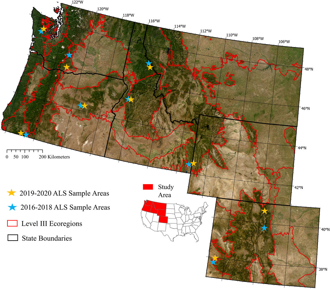
FIGURE 1. Western U.S. study region divided by EPA Level III Ecoregions with locations of validation ALS units designated by stars: orange stars depict validation collections for the years of model creation, and blue stars represent validation collections for years of model hindcasting.

2.2 Remote sensing model data

2.2.1 GEDI data

Forest wildlife habitat modeling efforts often include measures of forest height, canopy cover, foliage height diversity, and/or the availability of vegetation within specific strata of the forest (e.g., understory or upper canopy); these measures often correlate with important structure components necessary to meet life history needs for species, or to promote overall diversity of habitat niches (Bergen et al., 2009). After preliminary evaluations of available GEDI metrics in the context of frequently identified forest structure measures of value for habitat modeling purposes, we chose to focus our modeling efforts on several GEDI-derived height, cover, foliage height diversity, and summarized plant area density profile metrics corresponding to important habitat structure components for a variety of wildlife species. GEDI level 2A relative height (RH) metrics represent the height at which a defined percentage of GEDI waveform energy is contained. For instance, RH98 corresponds to the height at which 98% of the waveform energy is captured - comparable to a canopy height measure. We also included RH50 and RH75 within our modeling efforts to test their utility for wildlife modeling in future applied research efforts. Among the GEDI level 2B metrics, we selected two commonly used forest measures in wildlife habitat modeling, fractional canopy cover (COVER) and foliage height diversity (FHD). Among the Level 2B plant area vegetation density (PAVD) profile metrics, we choose the lowest single profile available through the GEDI waveform metrics that represents the 5–10 m strata (PAVD5-10 m), as well as summarizing plant area densities above 20 m (PAVD>20 m) and 40 m (PAVD>40 m) to represent the presence of a mature upper canopy within different forest types.

We leveraged the rGEDI package (Silva et al., 2020) implemented in the R Statistical Software (R Core Team, 2021) to download and filter GEDI version 2 footprint data across our study area. We restricted our target GEDI footprints within a summer season date range of June 6th - September 30th for both 2019 and 2020 to limit any bias in canopy cover and vegetation density profiles in mixed or deciduous forests outside of the primary growing season. We further filtered the summer season GEDI shots with a series of conditional arguments to retain only the highest quality observations to serve as model reference and testing data, including a solar elevation below 0°, a degrade flag of 0, a quality flag of 1, a beam sensitivity of greater than or equal to 0.95, and only employing full power beams. After filtering, the remaining GEDI footprints were intersected with the study area and each footprint observation was reprojected into an Albers Equal Area Projection (EPSG 5070).

While the rich spatial density of GEDI footprints provides value for a wide suite of applications including direct quantification and monitoring of forest patterns across broad extents, for our purposes in leveraging GEDI footprints as a model reference source, we chose to spatially thin our GEDI footprints to balance computational efficiency while maximizing model performance. We developed a set of spatial thinning steps to reduce the density of GEDI footprints while ensuring a spatially balanced sample across our study area. We first took a random subsample of 150,000 observations for each year. Constructing a set of polygon tiles with a 60 × 60-km resolution over the desired study region, we generated a Euclidean distance matrix for the subsetted footprints within each tile. Based on the distance between each footprint, 225 maximally distanced footprints were retained per 3,600 square kilometers. The resulting spatially subsetted dataset consisted of 99,766 observations for 2019 and 100,003 observations for 2020.

2.2.2 Continuous remote sensing predictors

We leveraged the computational efficiency of Google Earth Engine (GEE) to generate a suite of 31 active and passive remote sensing predictor layers for upscaling GEDI forest structure metrics to a continuous 30 m resolution grid and to apply models at annual time steps from 2016–2020. We wanted to test the utility of GEDI-fusion models for hindcasting structure metrics to years outside model creation, but were restricted to the 2016 forward time period due to the temporal availability of Sentinel-1 data included within our data fusion assessments. All dynamic predictors (e.g., Sentinel-1 and Landsat) were summarized for the summer growing season to match the temporal window of our GEDI data. From median summer composites of the Sentinel-1 C-band Synthetic Aperture Radar (SAR) dataset, we compiled the vertical-vertical (VV) and vertical-horizontal (VH) polarizations along with several ratios derived from the median VV and VH data including:

$VHVVratio=VH/VV$

$normalizeddifferenceradarindex=\frac{\left[VV-VV\right]}{\left[VH+VV\right]}$

$radarvegetationindex=\frac{\left[4*VH\right]}{\left[VV+VH\right]}$

For our Landsat spectral predictors, we created Medoid image composites for the annual summer seasons for the full Landsat archive (1984–2021), from which annual spectral indices were then calculated. Studies have found that when forest attribute models are created for a particular time period and then applied across a longer time period, using a temporal segmentation fitting algorithm can aid in producing more stabilized temporal representations of the modeled attribute within predicted maps (Moisen et al., 2016; Kennedy et al., 2018a). We used one such trend fitting algorithm, LandTrendr in GEE (Kennedy et al., 2018b), to calculate vertices within each spectral index and the original bands to produce annual “fitted” values for all Landsat predictors (Table 1). In additional to the original Landsat bands, we incorporated several Landsat spectral indices in our “fitted” Landsat predictor set that are commonly used within forest attribute modeling and change detection: tasseled cap brightness, greenness, and wetness (Crist and Cicone, 1984); the normalized difference vegetation index (Rouse et al., 1974); the enhanced vegetation index (Liu and Huete, 1995); and the normalized burn ratio (Key and Benson, 2006).

TABLE 1

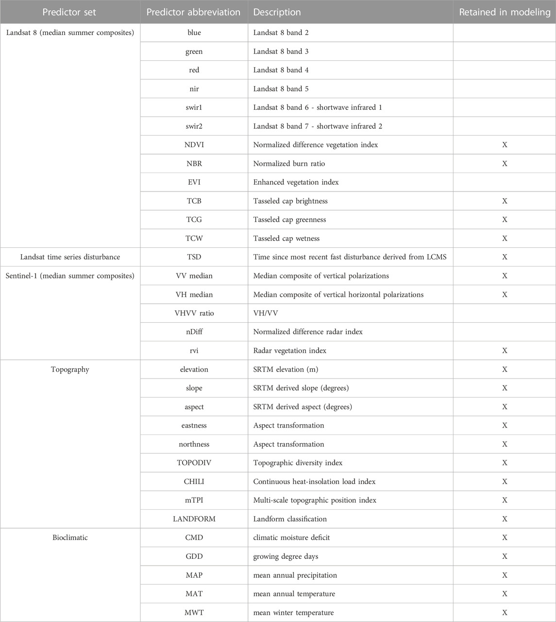
TABLE 1. Continuous predictor variables grouped by data source incorporated within GEDI-fusion modeling frameworks. Those predictors retained in final models after removing highly correlated variables within individual models sets are marked with an X.

While annual Landsat information may be correlated with some forest measures such as canopy cover (Coulston et al., 2012), previous research has highlighted the additional value of Landsat time series derived information of disturbance histories for improving structure predictions (Pflugmacher et al., 2012; Vogeler et al., 2016). To test for similar improvements, we generated a model predictor related to disturbance histories derived from the United States Forest Service Landscape Change Monitoring System (LCMS) dataset (Housman et al., 2022). We filtered the annual dataset to derive an image collection representing the most recent year of abrupt, or “fast”, forest change. We subtracted this most recent disturbance year from the year of interest (depending on the year of GEDI data or mapping year) to derive an annual raster layer indicating the number of years since the last fast disturbance (here forward referred to as time since disturbance, TSD).

To complement the dynamic spectral and SAR predictors and to represent the gradients that exist across our study area, we also extracted topographic and bioclimatic information (Table 1). Utilizing the Satellite Radar Topography Mission (SRTM) dataset, we calculated elevation, slope, aspect and aspect transformations (eastness and northness). We also incorporated additional topographic predictors based on SRTM including the Topographic Diversity Index (TOPODIV), Continuous Heat-Insolation Load Index (CHILI), Multi-Scale Topographic Position Index (mTPI), and landform classes created by combining CHILI and mTPI (LANDFORM) (Theobald et al., 2015). ClimateNA (version 7.2.1; Wang et al., 2016) was used to generate a set of bioclimatic variables derived from PRISM 4 km × 4 km gridded monthly climate for the 1961–1990 “normal” period (Daly et al., 2008), which were downscaled using the global 1-arcsecond v3 SRTM digital elevation model. We chose this “normal” period as it likely corresponds to the time when many of our mature forests were developing across our study area. More recent normals may provide an updated version of this data for the period impacting younger forest development, but we believe that the older versions are still appropriate for our purpose of representing relative differences in climatic gradients across our study region. The resulting bioclimatic variables included climatic moisture deficit, growing degree days, mean annual precipitation, mean annual temperature, and mean winter temperature (Table 1).

The spatial resolution of the processed predictor datasets varied from 10 m (SAR) to 270 m (some of the topographic position and diversity indices). All predictors were either aggregated or resampled to a common 30 m grid and exported from GEE for local modeling and predictive mapping using the EPSG 5070 projection within analysis ready dataset tiles. The spatially filtered GEDI locations for each year were buffered by 12.5 m to generate polygons representative of the 25 m diameter of the GEDI footprints. All above predictors were extracted using an area weighted mean pixel value from all pixels intersecting a footprint’s polygon, and for temporally dynamic predictors the year used for extraction corresponded to that of the GEDI footprint’s acquisition year.

2.3 GEDI-fusion modeling and mapping

A primary goal of our study was to test the utility of GEDI data as a reference source combined with various continuous predictor layers for scaling up structure information relevant to habitat modeling across continuous regional extents at 30 m spatial resolutions from 2016–2020. Different predictor data sources (e.g., Landsat, Sentinel-1) may have various tradeoffs as to model performance, spatial biases, and potential hind-casting capabilities. Thus, comparing different predictor sets can help inform the potential value and trade-offs of data fusion frameworks. All model accuracies and errors were assessed using a withheld set of testing GEDI footprints. Further spatial bias and temporal transferability were evaluated using our sample of ALS collections across two-time mapping windows representing years of model creation and model hindcasting (Figure 1; section 2.4.2). We completed an initial evaluation of random forest regression (Breiman, 2001) with progressively larger training samples to identify the number of training samples at which model performance began to stabilize for a sample set of GEDI metrics (i.e., a learning curve), and we used this number of training and testing samples for subsequent model development and evaluation.

We defined an a priori set of data fusion model combinations (Table 2) to compare model performances and spatiotemporal biases. Within each single-source predictor set (e.g., Landsat, topography), we first tested for highly correlated variables using a correlation threshold of 0.95. Only those not highly correlated were retained within the model comparisons (Table 1). The reduced variable sets were also combined to determine the best overall model for each GEDI metric in terms of model performance and errors as assessed using the withheld testing set of footprints. The fusion models representing the full set of predictors (combined model) and the model incorporating Landsat, topography, and bioclimatic predictors (Landsat/topo/bio model) were applied to the predictor layers to produce 30 m resolution maps of the GEDI metrics across the study area and on annual time steps from 2016–2020. As a final post-processing step, we developed an open-water mask using the Global Surface Water Layer v1.4 within GEE (Pekel et al., 2016), which we applied to all final maps to minimize false vegetation structure measures as a result of our GEDI filtering approaches that removed all water GEDI points; therefore, water bodies were outside the scope of our model reference data.

TABLE 2

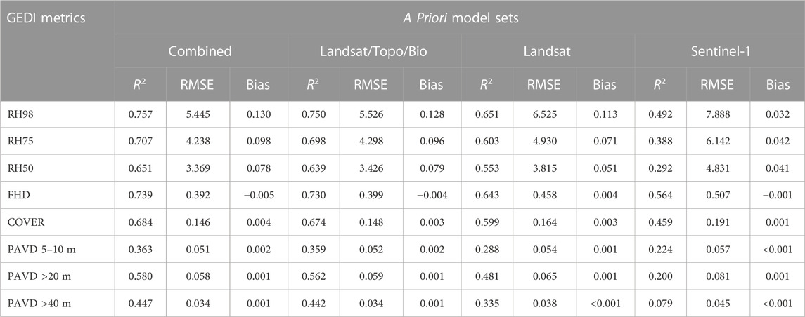
TABLE 2. GEDI-fusion model comparisons using a priori model predictor sets. All accuracy and error statistics calculated using a withheld testing set of ∼140,000 GEDI footprints. The combined model includes metrics from all predictor sets.

2.4 Validation assessments

2.4.1 GEDI Footprint-ALS comparisons

GEDI-fusion frameworks are based on the assumption that the information provided by the GEDI footprints are accurate representations of forest structure for serving as modeling reference data. To test this assumption and to inform sources of error in the GEDI-fusion maps, such as the potential for up to 10 m geolocation errors within the GEDI data, we compared footprint estimates of focal metrics to those from ALS samples. ALS data may be limited in spatial extents and temporal coverage, but the sources of errors and vertical/horizontal accuracies are well established and can serve as a baseline for comparisons with GEDI-derived forest measures and for comparing patterns in spatiotemporal biases between GEDI-fusion maps. We identified a set of ALS collections for the years of our GEDI footprint samples (2019 and 2020) that represent the forest-dominated ecoregions of the study area based on the EPA Level III Ecoregions (US EPA, 2015; Figure 1). The sample ALS collections also captured a wide range of forest structure variability and disturbance patterns. While our models and predicted maps encompass the extent of our six study states, the focal area for our habitat case studies were the forested regions of those states. As such, our ALS validation samples represent forest and shrubland cover types and our validations are only representative of forested lands in the region.

The majority of ALS data are collected using discrete lidar sensors, while GEDI is a full-waveform system. To convert the ALS measures to those comparable to waveform derived structure metrics, we employed the GEDI waveform simulator, gediSimulator (Hancock et al., 2019), frequently used within GEDI-ALS comparisons. That said, by simulating waveforms with discrete ALS, we acknowledge that we may be introducing some level of error within our validation data set although allowing for more direct comparisons of metrics than possible between waveform and discrete lidar. Within the selected ALS comparison units (Supplemental Table S1), we clipped the ALS point clouds at our filtered GEDI footprint locations corresponding to the year of ALS. Preprocessing the ALS clips involved identifying lidar returns within 60 cm of the ground surface and reclassifying those lidar returns as ground returns to account for topographic variations within a simulated footprint (Hancock, 2023). The gediSimulator tool, gediRat, was used to convert the ALS point clouds into a simulated waveform, which were passed to gediMetric to calculate waveform metrics. Simulated cover outputs are reported to be particularly sensitive to variations in topography within a footprint (Hancock, 2023), which can be significant within our study area. Implementing the suggested pre-processing steps for minimizing the impacts of topographic variations on ALS simulated metrics did not appear to improve the simulated cover metric for our sample ALS areas. Therefore, we chose to directly compare discrete ALS cover to our GEDI footprint and map cover estimates, although we acknowledge that slightly different measures of canopy cover may be represented by these two measures. We calculated the discrete ALS cover metric as the proportion of first returns above 2 m within the FUSION lidar processing software (McGaughey, 2022). We then compared the simulated or direct ALS-based metrics to the GEDI-based metrics for matching years (e.g., 2019 GEDI footprints compared to simulated 2019 ALS metrics) by calculating the coefficient of determination ($R^2$), mean bias ($bias$), and root mean squared error ($RMSE$). We were unable to include our PAVD metrics within the footprint and map level validations as these are not direct outputs available from gediSimulator (Hancock, 2023), nor are there readily comparable metrics from discrete ALS. Evaluations for the PAVD metrics were restricted to the prediction assessments from the large set of withheld testing GEDI footprints (described in section 2.3).

Many studies comparing simulated ALS waveforms to GEDI footprints conduct an additional step to better georeference the GEDI footprints based on the ALS information as GEDI version 2 footprints may have up to 10 m geolocation error. For our purposes, we wanted to directly compare GEDI footprints to ALS information without additional georeferencing steps to directly test the utility of footprints as reference data in areas where we do not have corresponding ALS data sets for location corrections. Therefore, some of the variability observed within our footprint level comparisons may be due to geospatial mismatches between the ALS data and the recorded footprint locations. As such, the comparisons are not intended as direct validations of the GEDI instrument measurements in the absence of geolocation errors, but instead validations of the footprint level information in their original form as a reference data source for scaling up structure information which may aid in understanding the errors observed within our resulting study-area wide GEDI-fusion predicted maps.

2.4.2 Structure map validations

In addition to comparing model performance through the withheld set of independent GEDI footprints, we also evaluated biases within the predicted maps and temporal transferability of models. We leveraged our sample set of ALS units for years of model creation (2019–2020) and a set of ALS collections from 2016–2018 to represent years of model hindcasting to evaluate differences in map accuracies when models were applied to years outside of the model training data (Supplemental Table S1). We ensured that the sampled collections within both time windows were representative of the range of forested ecoregions within our study area (Figure 1).

Maps of simulated gridded waveform metrics within the ALS sample units were created using a similar approach as outlined for footprint level comparisons above (section 2.4.1). PDAL (PDAL, 2022) was used to filter ALS lidar in the sample units to include only ground and vegetation returns, as well as reclassifying all returns within 60 cm of the ground surface as ground returns. The preprocessed ALS files were then converted to simulated waveforms and waveform metrics (Hancock, 2023). Following our same comparison approach for cover measures as used in our footprint-level comparisons, we utilized a gridded ALS cover measure created within FUSION representing the proportion of first returns above 2 m (McGaughey, 2022). The size of the ALS collections used in the comparisons ranged between 150 and 450 km² (Supplemental Table S1), therefore a random sample of 1,100 cells were drawn from each ALS unit for a total of 9,900 pixels selected during the years of creation (2019–2020) and 9,900 pixels from hindcasted years (2016–2018). We created scatterplots of the map validation sample points for each time period, as well as calculating R², bias, and RMSE for each temporal validation dataset.

2.5 Case study: wildlife habitat modeling

Primary cavity excavators are considered a keystone wildlife guild because they excavate tree cavities that provide nesting and roosting habitat for multiple other species who cannot excavate those cavities themselves (Martin et al., 2004; Gentry and Vierling, 2008; Tarbill et al., 2015). For instance, Bunnell et al. (1999) noted that 25%–30% of vertebrates within Pacific Northwest forests are reliant on woodpecker cavities for either nesting or roosting, and many of these secondary cavity users are themselves species of management interest (e.g., fishers (Pekania pennanti) and marten (Martes spp.); Bissonette and Broekhuizen, 1995; Matthews et al., 2019). We chose three cavity excavator avian species which occur within our study region and are associated with different forest structural elements. These include the downy woodpecker (Dryobates pubescens), the Northern flicker (Colaptes auratus), and the pileated woodpecker (Dryocopus pileatus). Downy woodpeckers are small woodpeckers that prefer deciduous forest elements, small trees, and low canopy cover (Jackson et al., 2020). Conversely, pileated woodpeckers are associated with more mature forest elements, particularly tall trees (Bull and Jackson, 2020). Northern flickers are intermediately sized between the other two woodpecker species, and are associated with forest edges (Wiebe et al., 2017).

We followed best practices (Johnston et al., 2019; Strimas-Mackey et al., 2020) to obtain pileated woodpecker, Northern flicker, and downy woodpecker observations from eBird records (eBird, 2021). As a general workflow, we obtained stationary eBird checklists conducted in the study area between June 1 and July 31 of 2016–2020. For pileated woodpeckers, we restricted checklists to those taking place at longitudes west of −108.723868°, to account for the limited range of this species in the study area. Northern flicker and downy woodpecker occur throughout the study area and therefore checklists for these species were not restricted by longitude. After spatiotemporal subsampling (following Strimas-Mackey et al., 2020), we obtained the effective sample size for positive observations for each species and retained 20% of the data for model evaluation. We selected modeling scales based on estimated home range sizes for each species. We used a 250 m radius buffer size for downy woodpeckers (Jackson et al., 2020), 500 m radius buffers for Northern flickers (Wiebe et al., 2017), and a 1 km radius buffer size for pileated woodpeckers (Bull and Jackson, 2020). In random forest regression models, we used the observations for each species as our response variables and the following predictor variables: survey particulars (survey duration and time of day); forest type (confer, deciduous, or mixed) from MODIS data (Friedl and Sulla-Menashe, 2015); elevation, slope, eastness and northness from SRTM; and our set of GEDI-fusion maps produced as explained above. We first generated models for each woodpecker species using the GEDI-fusion layers created from the combined model and then repeated the process for each species using only the restricted Landsat/topo/bio model outputs. This direct comparison allows us to ascertain how models with different accuracies and biases affect wildlife model outputs.

3 Results

Overall, our data fusion approaches leveraging GEDI footprint forest structure information and continuous remote sensing data sources proved valuable for producing regional extent gridded maps of forest architecture with moderate to high model performances which were of value to wildlife habitat assessments for three cavity nester species representing different forest structure associations. Specific data, modeling, and mapping validations are presented below.

3.1 GEDI-fusion model assessments

Model performance stabilized at approximately 60,000 training footprints in our initial model testing, which was the sample size used for subsequent model development along with a withheld set of approximately 140,000 footprints for model testing. All reported model accuracies and errors were quantified using the independent testing set of footprints.

Our random forest combined models predicting GEDI structure metrics from continuous satellite remote sensing data sources had high model performance for the majority of the GEDI metrics. Within the combined models incorporating all predictor data sources, the highest performance was observed for RH98 (R² = 0.76, RMSE = 5.46 m) and FHD (R² = 0.74, RMSE = 0.39). Lower model performances were observed for the PAVD metrics, with R² values ranging from 0.36 (PAVD5-10 m) to 0.58 (PAVD>20 m), and RMSE values ranging from 0.03 (PAVD>40 m) to 0.06 (PAVD>20m; Table 2). The performance of the Landsat/topo/bio models were only slightly lower than that of the combined model for all GEDI metrics (Table 2). When comparing the single source Landsat model to the Sentinel-1 model, the Landsat model exhibited higher model performance for all metrics (Table 2). These differences in performance for the single source predictive models were the lowest for FHD, COVER, and RH98, in that order.

When comparing relative importance of predictor variables within the combined random forest models, Landsat variables were common among the top five most important predictors for all GEDI metrics (Table 3). Sentinel-1 metrics were also within the top five predictors for most GEDI metrics, and within the top ten predictors for all GEDI metrics apart from FHD (Table 3). Disturbance information (TSD) was only among the top ten predictors for PAVD>20 m. Topography and bioclimatic variables were among the top ten predictors for all GEDI metrics, and among the top five for FHD and the PAVD metrics (Table 4), representing the importance of macro (bioclimatic) and micro (driven by topographic patterns) climatic gradients on driving vegetation within particular forest strata as well as for promoting overall diversity of the vertical vegetation profile.

TABLE 3

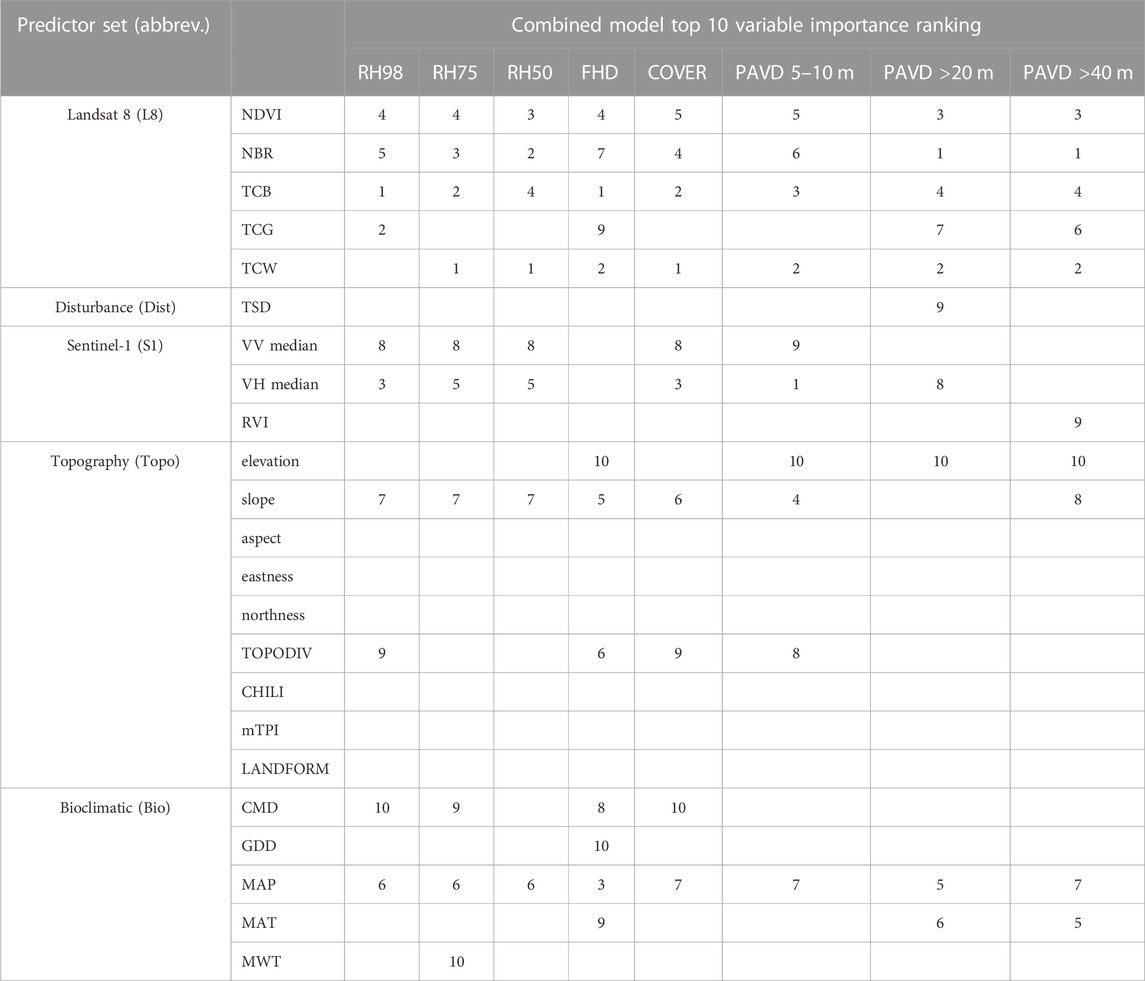
TABLE 3. Random forest variable importance rankings for the top 10 predictor metrics within the combined models for GEDI-fusion metrics.

TABLE 4

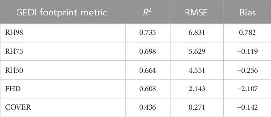
TABLE 4. Comparison statistics for GEDI Level 2A and 2B footprint metrics and ALS metrics for a sample of ALS units across our study area. Simulated waveform metrics from ALS were used for all comparisons with the exception of COVER, which was produced directly from discrete ALS data (proportion of first returns above 2 m). Validation results are not included for PAVD metrics as those are not available as outputs from the GEDI simulator or directly from discrete ALS. RMSE units are in meters for relative height (RH) metrics and proportions for COVER. FHD is unitless.

3.2 Validation assessments

3.2.1 GEDI footprint- ALS comparisons

Comparisons between ALS simulated (RH and FHD metrics) or direct discrete ALS measures (COVER) to those from GEDI footprints showed variability in accuracies across the GEDI metrics (Table 4). We observed the highest comparison accuracies for RH98 (R² = 0.74, RMSE = 6.83 m) and the lowest accuracies for COVER (R² = 0.44, RMSE = 0.27). The remaining height metrics of RH75 and RH50 along with the FHD metric had comparable accuracies, with R² values of 0.70, 0.66, and 0.61, respectively. The majority of the metrics had a negative bias with the exception of RH98, which means that the GEDI footprints tended to underestimate values compared to ALS measures. The simulated FHD values exhibited a systematic bias in that they had a higher range of values to those from the GEDI footprints (bias = −2.107), but still exhibited a good validation comparison with the actual GEDI footprint values (Table 4). The lower model performances observed between the GEDI and direct ALS cover measures may be influenced by a multitude of factors; these include the different representations of cover within waveform vs discrete lidar measures of cover, geolocation errors within the GEDI footprints, or issues with the ground finding algorithm within the GEDI footprint influencing the resulting cover estimate.

3.2.2 Structure map validations

Through our GEDI-fusion frameworks, we were able to successfully scale up GEDI structure information to continuous extents, capturing horizontal and vertical structural patterns across our six-state western U.S. study area (Figure 2). Our results show variability in map performance across the GEDI-fusion metrics although all had moderate to high predictive performance (R² = 0.59–0.75; Table 5). Map accuracies and errors were comparable between maps within years of model creation to those representing hindcasted years for both the combined and Landsat/topo/bio models (Table 5). Map accuracy was only slightly higher from the combined model than from the Landsat/topo/bio model for all GEDI-fusion metrics (Table 5). The comparable accuracies and errors between the model-map versions and the consistency between years of model creation to hindcasted years, show promise for the potential of further map hindcasting using the Landsat/topo/bio model prior to years of Sentinel-1 data. From here forward we focus on map validation results for the combined model-based maps for the years of model creation.

FIGURE 2

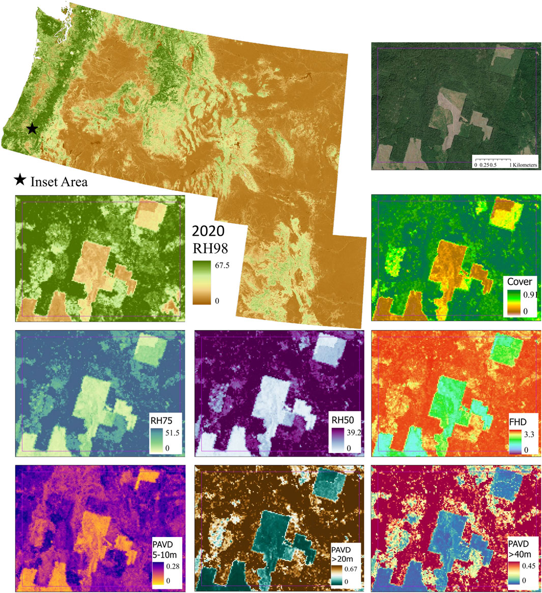
FIGURE 2. GEDI-fusion RH98 2020 map across our 6-state study area with an example inset area showing 2020 maps of the full set of GEDI-fusion maps created using the combined model (RH98, RH75, RH50, FHD, COVER, PAVD 5–10m, PAVD >20m, and PAVD >40 m). All height metrics are in meters, COVER and PAVD metrics are proportions, and FHD is unitless.

TABLE 5

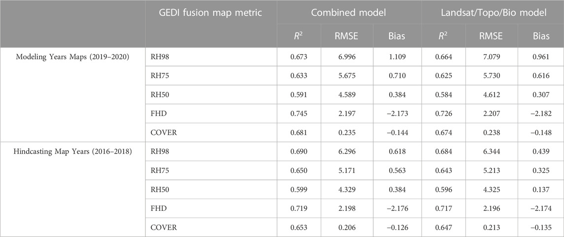
TABLE 5. GEDI-fusion gridded predicted map validation with GEDI-simulator ALS (or direct discrete ALS for COVER) sample units for maps created with the combined predictor model and the Landsat/topo/bio model. Validation results are not included for PAVD metrics as those are not available as outputs from the GEDI simulator used to simulate comparable waveform metrics from the ALS sample units, or through direct discrete ALS measures.

Among the GEDI-fusion metrics, FHD had the best map accuracy (R² = 0.745), although it still exhibited the systematic bias observed within the footprint level comparisons (Figure 3). RH50 had the lowest map accuracy with an R² of 0.59 and RMSE of 4.59 m (Table 5) and map predictions underestimated RH50 compared to simulated values, particularly among higher RH50 simulated heights (Figure 3). The order of validation performance rankings of the GEDI-fusion metrics was different between the footprint- and map-level validations, but the general range of accuracies and errors and moderate-high performance was consistent between scales of analyses (Tables 4, 5).

FIGURE 3

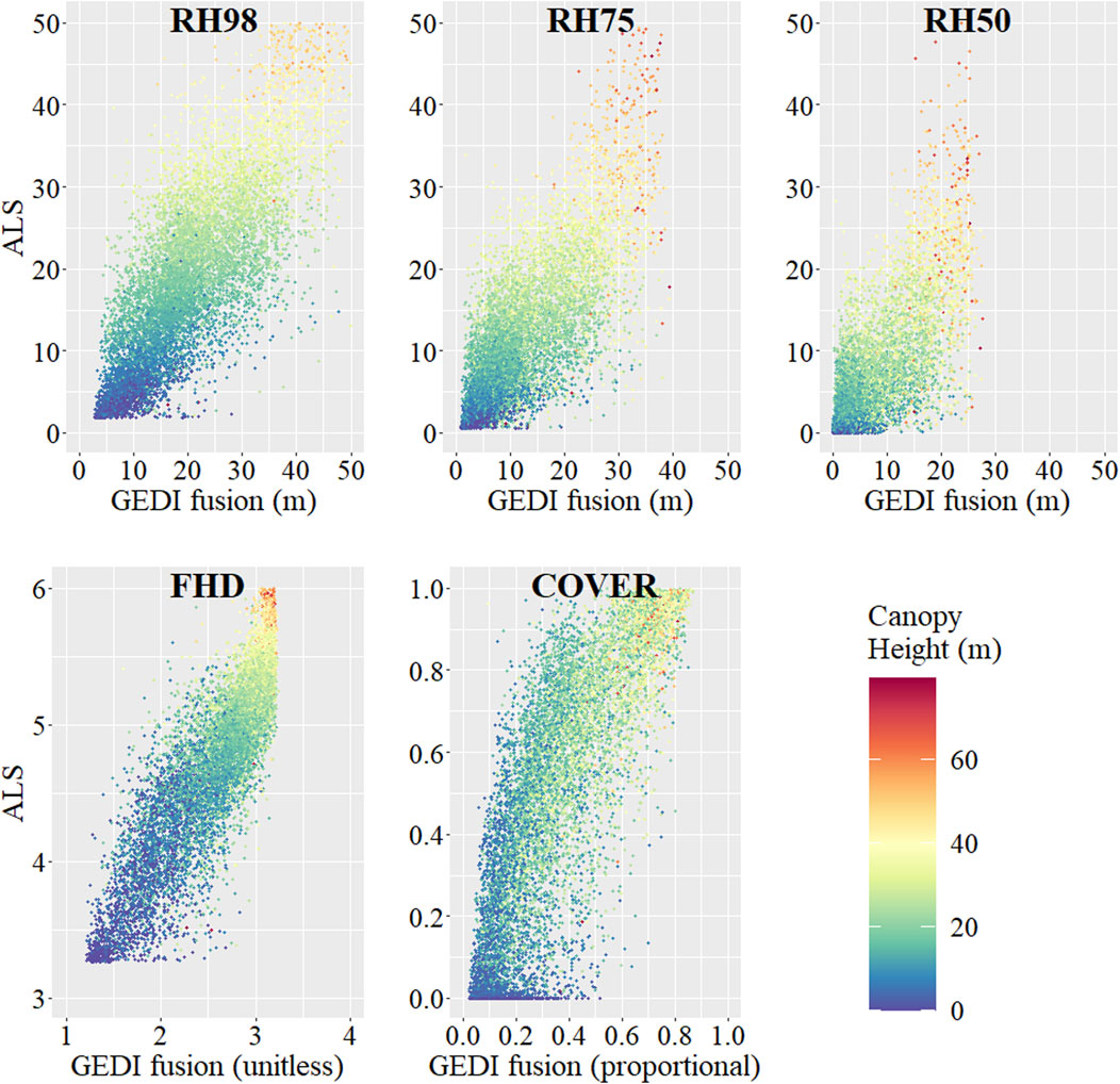
FIGURE 3. Scatterplots of the predicted GEDI-fusion metrics maps (GEDI-fusion) compared to simulated waveform grids (or direct discrete ALS grids in the case of COVER) for our validation ALS units (ALS) for a random sample of validation pixels. Relationships shown are those for the combined model GEDI-fusion maps and for map years and ALS units representing years of model creation (2019–2020). Scatterplot color scale depicts discrete ALS-derived maximum canopy height.

3.3 Case study: wildlife habitat modeling

Our GEDI-fusion maps show promise for supporting large extent forest wildlife habitat modeling efforts according to the results of our case study, which focused on three species representing different forest structure associations and home range scales. We were able to successfully model habitat for our three cavity-nesting avian species with “good” performance according to AUC values (Swets, 1988) by incorporating structure information provided by the GEDI-fusion maps (Table 6). Habitat models for the pileated woodpecker exhibited the highest AUC values, closely followed by the downy woodpecker, and then the Northern flicker (Table 6). In general, the habitat models had very high specificity with lower sensitivity (Table 6), meaning that the maps were better at predicting areas where the species were not encountered than areas where they were present.

TABLE 6

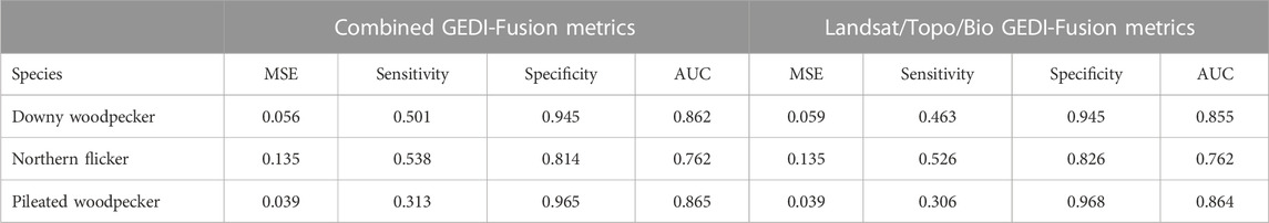
TABLE 6. Comparison of habitat models for three case study wildlife species that incorporate the GEDI-fusion metrics from either the combined model or the Landsat/topo/bio model. Model assessment statistics include the mean square error (MSE), sensitivity, specificity, and area under the curve (AUC).

When comparing habitat models incorporating the two different GEDI-fusion mapping versions, we observed minimal differences for all species, with only slightly higher (or directly comparable) AUC values for the habitat models incorporating the GEDI-fusion metrics from the combined models compared to those from the Landsat/topo/bio fusion maps (Table 6). The two versions of the random forest habitat models for each species also had similar ranking for relative importance of predictors (Table 7), so here forward we will only discuss the habitat models incorporating the GEDI-fusion metrics from the combined fusion maps. Following eBird habitat modeling best practices, we incorporated variables within our models related to survey timing and durations. Not surprisingly, both metrics were among the top five predictors for all three species (Table 7). There was a greater probability of detecting an individual of the species earlier in the day when birds are known to be more active and vocal, and as survey durations covered longer periods of time (Figures 4–6). Likewise, measures of topography were included in the top 9 predictors for all three species. Elevation was particularly important for downy woodpecker, for which it was the single most important variable (Table 7). Slope was in the top 7 predictors for downy woodpecker and Northern flicker, but not for pileated woodpecker (Table 7).

TABLE 7

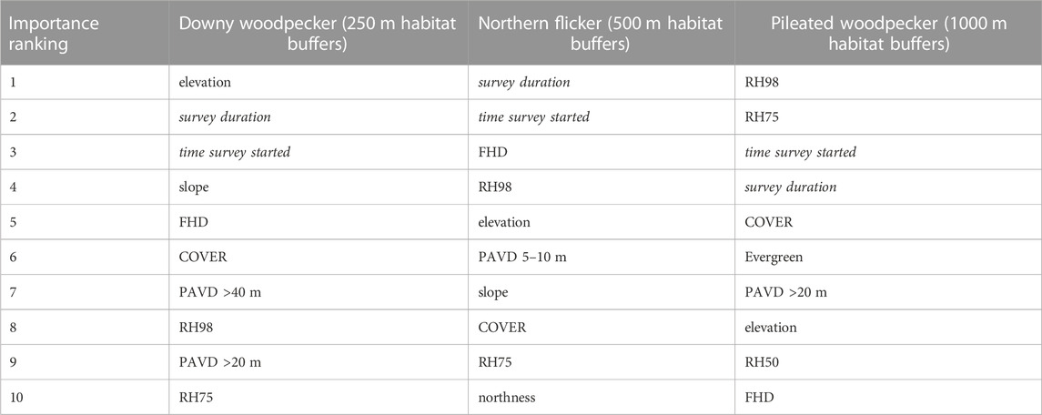
TABLE 7. Random forest variable importance rankings for the top 10 predictor metrics within the wildlife case study habitat models using the GEDI-fusion metrics from the combined models. Survey detectability related predictors are italicized as they are not related to environmental occurrence drivers.

FIGURE 4

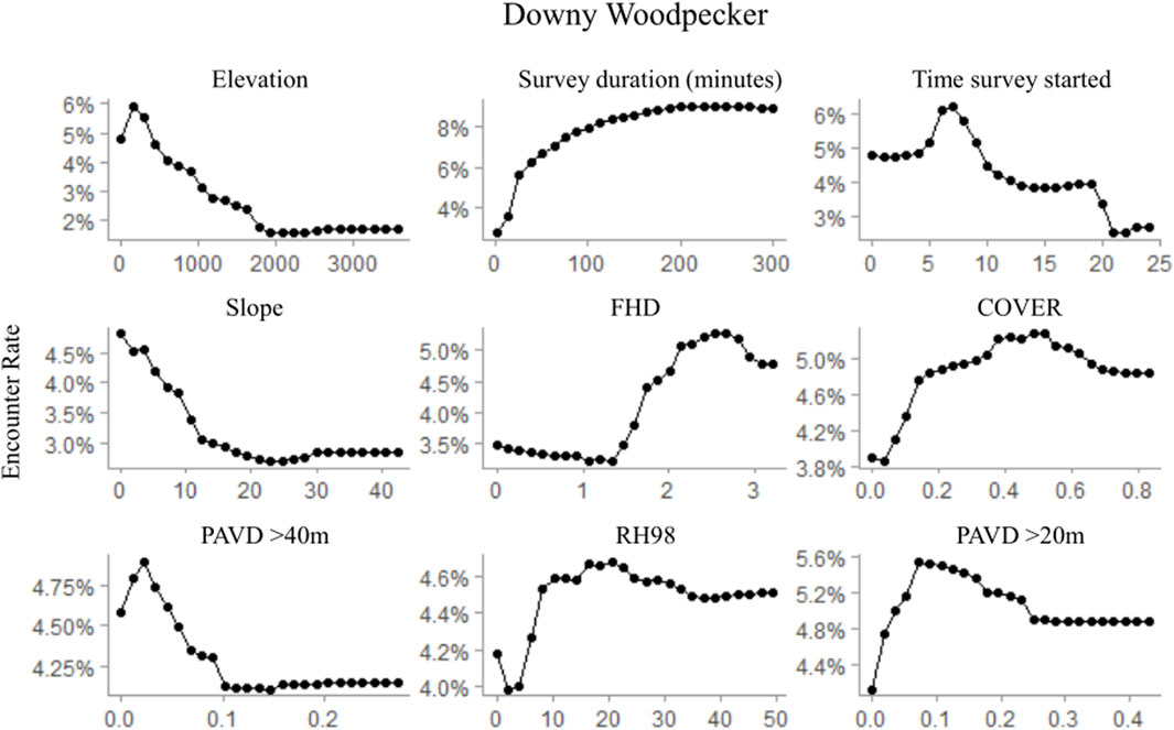
FIGURE 4. Partial dependence plots for the top nine ranked variables within the random forest downy woodpecker occurrence model depicting observed habitat relationships for GEDI-fusion, topographic, and survey timing metrics. Occurrence was modeled at a 250 m radius scale, comparable to the species average home range size.

FIGURE 5

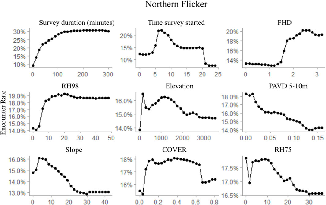
FIGURE 5. Partial dependence plots for the top nine ranked variables within the random forest Northern flicker occurrence model depicting observed habitat relationships for GEDI-fusion, topographic, and survey timing metrics. Occurrence was modeled at a 500 m radius scale, comparable to the species average home range size.

FIGURE 6

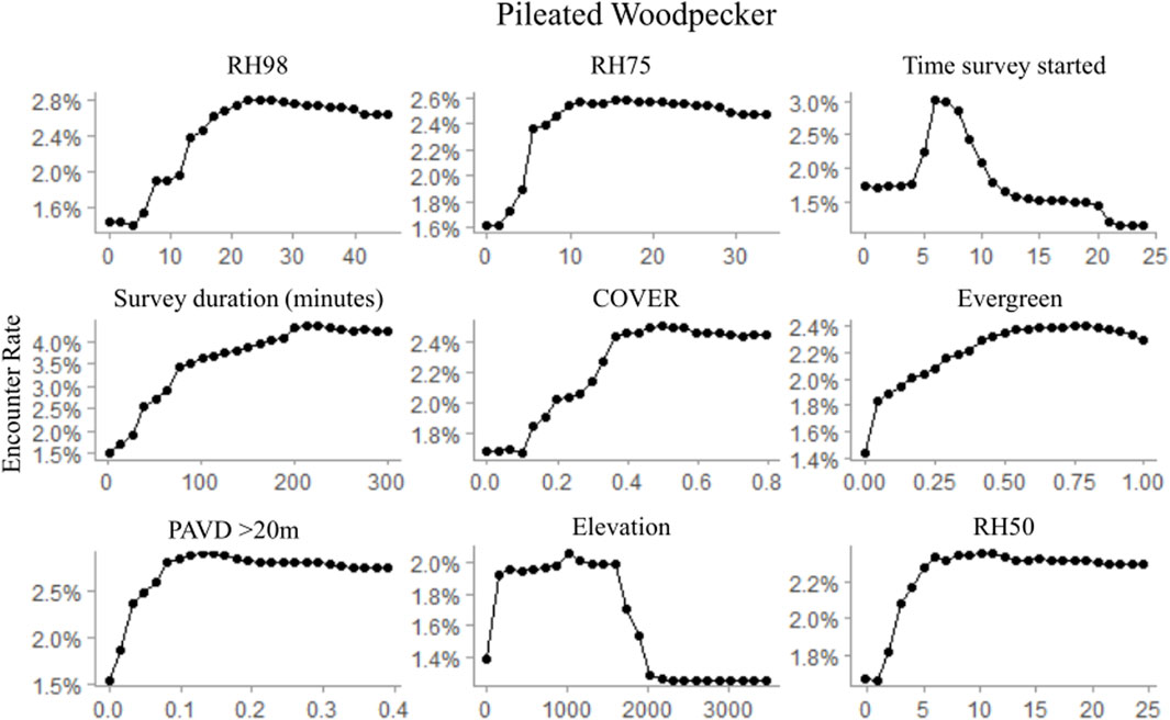
FIGURE 6. Partial dependence plots for the top nine ranked variables within the random forest pileated woodpecker occurrence model depicting observed habitat relationships for GEDI-fusion, topographic, and survey timing metrics. Occurrence was modeled at a 1,000 m radius scale, comparable to the species average home range size.

Regardless of the importance of topography and survey characteristics on detecting an occurrence for the species, GEDI-fusion metrics were also included among the top five most important variables for all species (Table 7). FHD was the most important GEDI-fusion metric for both downy woodpecker and Northern flicker, but was not ranked in the top ten variables for pileated woodpecker (Table 7). Both species showed higher encounter rates at higher FHD (Figures 5, 6). RH measures were particularly important for pileated woodpecker, with RH98 and RH75 ranked as the two most important variables overall and RH50 as the ninth most important variable (Table 7). All three species had highest encounter rates at high RH98 (Figures 4–6). Pileated woodpecker had the highest encounter rate at RH75 > 10 m (Figure 6), while Northern flicker encounter rate was negatively correlated with RH75 (Figure 5). COVER was ranked in the top eight variables for all three species (Table 7). For pileated woodpecker, encounter rate was highest at high COVER (Figure 6), while downy woodpecker and Northern flicker encounter rates peaked at moderate COVER (0.4–0.6; Figures 4, 5). PAVD metrics were included in the top 6–9 predictors for each species, but the strata of greatest importance were different across the species (Table 7). Downy woodpecker encounter rates peaked at low values (<0.05) of PAVD> 40 m and at PAVD>20 m values of approximately 0.1 (Figure 4). Northern flicker encounter rates were negatively related to PAVD5-10 m (Figure 5). Pileated woodpecker encounter rates were positively related to PAVD>20m, but reached an asymptote at PAVD>20 m values of approximately 0.1 (Figure 6).

4 Discussion

With the novel source of three-dimensional data provided by GEDI, it is critical to determine the advantages and drawbacks for use in modeling forest structure across a variety of forest types and architectures. Our study calibrated and tested predictive models across six western U.S. states with a variety of forest types across a bioclimatic gradient from the wetter coastal forests in western Washington and Oregon to the dryer southwest forests and woodlands of Colorado. Within our model assessments, we found moderate to high predictive performance for a set of eight GEDI structure metrics across our diverse study region. Much of the existing GEDI literature has focused on accuracy assessments of the GEDI waveform geolocations and structure measures (Adam et al., 2020; Li et al., 2023), developing footprint level biomass models (Duncanson et al., 2022), or leveraged simulated GEDI data in lieu of actual footprint samples (Burns et al., 2020; Silva et al., 2021). Studies have begun to investigate GEDI footprint samples as the basis for scaling up forest structure measures by leveraging fusions of passive and active satellite earth observations, although the majority of those studies have been focused on elevation, canopy height, or biomass (Healey et al., 2020; Potapov et al., 2021; Shendryk, 2022). Our comparison of additional GEDI metrics to ALS and our evaluation of the trade-offs between different data fusion frameworks provides valuable information on the potential of using GEDI data fusions to provide wall-to-wall structure information across different forest types for metrics useful in wildlife applications. While ALS-validation results within this study varied slightly between the footprint- and map-level assessments, moderate to high performances were observed for all metrics and the general range of accuracies and errors were consistent between scales of analyses. The consistency between footprint- and map-level assessments further supports the promise of data fusion approaches for scaling up GEDI structure information to continuous extents, even with geolocation errors from both GEDI footprints (e.g., up to 10 m error within version 2 GEDI data) and satellite predictors (e.g., potential of 15 m error for Landsat pixels).

Among the studies focused on scaling up GEDI structure metrics through data fusion approaches, the majority have largely focused upon GEDI canopy heights (Healey et al., 2020; Sothe et al., 2022; Ngo et al., 2023). Similar to these previous studies, we found high accuracies within our maps scaling up RH98 samples to continuous extents through optical and radar-based data fusions with an R² of 0.673 and RMSE of 6.996 m when compared against simulated ALS validation samples, and an R² of 0.757 and RMSE of 5.445 m when assessed using withheld GEDI footprint testing data. Healey et al. (2020) found progressively improved predictions of RH98 when global-extent models were calibrated within blocks of decreasing sizes, with optimization at 3 km. At this 3 km local calibration scale, they were able to achieve an RMSE of 7.08 m for RH98 predictions using only Landsat predictors across global-extents (Healey et al., 2020), which shows promise for the potential of expanding GEDI structure measures to larger extents than included in our regional study. Within sample tropical forest sites in South America and Africa, Ngo et al. (2023) found the greatest modeling success with RH98 among the possible upper canopy height GEDI metrics, supporting our inclusion of this variable. Similar to our results, Ngo et al. (2023) also found optical data the most important predictors of RH98 even when radar was included, with a validation R² of 0.62 and RMSE of 5 m when compared to an ALS canopy height. All previous studies of scaled-up GEDI RH98 predictions reviewed here had similar biases to those from our study, with under predictions at taller heights and over predictions at lower RH98 values (Healey et al., 2020; Sothe et al., 2022; Ngo et al., 2023).

To our knowledge, our study represents one of the first studies to extend GEDI data fusion evaluations to additional structure metrics beyond canopy height and biomass across regional extents, such as FHD and PAVD metrics. The novelty of these additional metrics at moderate resolutions across broad extents are likely to be extremely informative for wildlife focused studies. FHD has long been noted to be an important driver of local bird diversity patterns (e.g., MacArthur and MacArthur, 1961). Furthermore, wildlife species are sensitive to the density of vegetation within different height strata. For instance, a dense upper canopy is important for Pacific marten (Martes caurina), which are one of many forest mustelids of management interest (Buskirk and Ruggiero, 1994). Scaling up these metrics and producing continuous data layers is an important first step to explore structural characteristics that are likely to influence wildlife-habitat relationships.

Our results showed promise for applying GEDI-fusion models further back in time than our study period starting in 2016, where we found comparable map validation results for hindcasted years versus years of model creation for all structure metrics. We also found comparable performance for models based on Landsat, topographic, and bioclimatic predictors compared to the model that also incorporated Sentinel-1 and disturbance metrics, which supports the findings of Ngo et al. (2023) for the importance of optical data for scaling up GEDI information to continuous extents. The reliance on Landsat data for driving our GEDI-fusion models provides the opportunity to hindcast models further back across the Landsat archive prior to the availability of Sentinel-1 data. In addition, we compared the performance of the two GEDI-fusion map sets (one incorporating all predictors and the second only leveraging Landsat, topography, and bioclimatic predictors) within our wildlife habitat models for three case study species representing different forest structure associations. For all species, we found comparable habitat model performance between the two GEDI-fusion map sets. While Sentinel-1 data are likely to be helpful for wildlife modeling in multiple contexts (e.g., Koma et al., 2022), its exclusion from our GEDI-fusion models did not have downstream effects on wildlife modeling applications. Future studies expanding the time series of hindcasted GEDI-fusion models will require additional validation for the expanded temporal scope outside that of our study, as well as for implications within ecological applications.

The description of vegetation characteristics across broad extents, including vertical and horizontal structure patterns, is critical for managing and conserving wildlife species, since vegetation characteristics provide food, cover, and thermal resources for these organisms. While previous remote sensing-based wildlife habitat modeling efforts have shown value in the use of direct spectral indices from Landsat (Oeser et al., 2020), Sentinel-2 (Valerio et al., 2020), and MODIS (Viña et al., 2008), there is added applicability for habitat characterizations based on structure measures to meet the needs of forest managers who often manage their land in terms of across, or within, stand structure goals. When realized habitat relationships based on structural components can be mapped across the landscape as well as through time (Davies and Asner, 2014; Eitel et al., 2016), there are also opportunities for monitoring changes in habitat availabilities and connectivity through time, or to better match the timing of habitat variables with the timing of wildlife surveys. The annual maps of structure components for 2016–2020 which we produced here were successful in characterizing habitat for our three case study species. We were able to do so leveraging citizen science wildlife survey data sets (i.e., eBird data), where the multiple years of GEDI-fusion maps facilitated the matching of survey years to habitat predictors across multiple years, increasing our records. eBird data are now widely used in studies addressing bird distributions, movements, and diversity hotspots (e.g., Sullivan et al., 2014), and while a limited number of studies to date have included eBird data with GEDI data (Burns et al., 2020, this study), we anticipate that investigations of bird populations and communities that use scaled up, continuous GEDI-fusion data are likely to be of great benefit to the conservation and management of birds given their sensitivity to forest structure.

Important to the mapping of animal habitat are considerations of scale. Animals select their habitat at hierarchical scales from the species’ geographic range down to the foraging and cover resources an individual utilizes within their territory (Johnson, 1980), and different species operate at different spatial scales. Spatially continuous representations of fine-moderate resolution vertical and horizontal forest structure and patch characteristics facilitate the simultaneous evaluation of multiple scales of habitat selection for different species (Holbrook et al., 2017), as well as the mapping of realized wildlife habitat relationships across the landscape (Lesmeister et al., 2019), providing valuable forest planning tools. Our study included three species with home ranges that ranged from 2 ha (downy woodpecker; Jackson et al., 2020) to approximately 400 ha (pileated woodpecker in Oregon; Bull and Jackson, 2020), and our analyses resulted in AUCs of 0.76–0.87, suggesting that the GEDI-derived structure data were successfully reflecting habitat elements. This finding is consistent with Smith et al. (2022), who found that GEDI-derived metrics were important for modeling a suite of mammal species that operated at different spatial scales (e.g., snowshoe hares (Lepus americanus) and coyotes (Canis latrans)). In general, our habitat models had very high specificity with lower sensitivity, meaning that the maps were better at predicting areas where the species were not encountered than areas where they were present; this is common within modeling of wildlife occurrence as a number of non-environmental factors may influence the occupancy of a suitable patch by an individual of a species, including inter- and intra-species competition, predator-prey dynamics, and population densities.

The GEDI metrics used in this study were hypothesized to reflect important forest structural elements for our selected species, and our findings suggest that the GEDI-fusion data were successful in representing those elements. For instance, pileated woodpeckers require large trees for nesting and roosting (Bull and Jackson, 2020), and our results that RH98 were positively associated with the species encounter rates are consistent with pileated woodpecker ecology. Northern flickers often forage at the edge of stands while nesting in large trees (Wiebe et al., 2017), and the positive relationship of this species with increasing levels of RH98 and FHD are again consistent with their nesting and foraging ecology. Burns et al. (2020) found that simulated GEDI data captured structural elements important for multiple bird species, and Smith et al. (2022) similarly found that GEDI-derived structural elements were important in improving distribution models of several mammal species. These studies, in addition to our findings, suggest that GEDI data represent structural elements at spatial scales that are important to a wide variety of wildlife species.

Beyond characterizing wildlife habitat, the remote sensing data fusion frameworks which we developed and tested for scaling up GEDI-based structure information to continuous regional extents may additionally provide value for other forest assessments. For instance, maps of forest structure components, such as height, canopy cover, and vegetation profiles, are also valuable for estimating biomass (Hudak et al., 2012) and forest management planning. In turn, this forest information may also serve as the basis for studies assessing the tradeoffs between managing for carbon sequestration, timber production, species specific habitat, and overall biodiversity (Kline et al., 2016). Understanding spatial forest structure patterns can also aid in calibrating forest projection models for predicting impacts of land use and management practices, as well as climate change scenarios, on future forested systems (Fekety et al., 2020) and habitat availability. Our focus on the use of only publicly available remote sensing products within our data fusions also ensures the applicability of our developed methods across other regions around the globe and within projects or programs with limited financial resources.

While some countries, such as the United States, benefit from federally funded periodic and systematic forest sampling efforts, including the U.S. Forest Inventory and Analysis (FIA) program, many developing countries do not have comparable forest monitoring programs. These countries contain some of the forests and biodiversity hotspots experiencing the greatest rates of anthropogenic driven land conversions and other threats to forest health and function (Jetz et al., 2007). Such areas could greatly benefit from a consistent forest structure sampling data set, such as GEDI, for regional assessments and monitoring, or to serve as reference data in modeling approaches such as those presented in this study to predict forest structures across continuous extents at resolutions relevant for a diversity of ecological applications. Even within valuable field sampling programs such as FIA, there are drawbacks for serving as reference datasets for some spatial modeling applications because of the need for meeting data security protocols which can restrict their use within cloud computing workflows and through their view of the forest from the ground up with variable georeferencing accuracies (e.g., inconsistent GPS sampling errors across regions and plots). GEDI shows promise for filling this data gap for consistent, 3-dimensional characterizations of the forest strata as measured from above, and publicly available at near global extents (Dubayah et al., 2020). While these data may provide a novel data source in many regions of the world, the rich density and availability of ALS collections along with the diverse gradients of forest types and climatic gradients still make the U.S. a valuable location to test the utility of GEDI for driving such modeling efforts and for validating spatiotemporal biases of the resulting products.

5 Conclusion

The purpose of our study was to test the suitability of the rich reference source of structural information that GEDI footprints provide within various data fusion modeling frameworks for scaling up metrics of value to wildlife habitat modeling applications. We conducted this assessment across broad extents at 30 m resolutions that are of value to a variety of forest assessments. We chose to conduct our analyses within the diverse western U.S. where there were corresponding samples of ALS data for validation purposes. This evaluation was intended to provide insights into the strengths and limitations of the resulting predicted structure maps across a variety of forest types and structures, to better inform similar mapping efforts within regions which do not have ALS samples or forest inventory programs. Since our goal was to use computationally approachable workflows, we filtered and spatially thinned our GEDI footprints to a sample size that balanced model accuracy with computational needs. However, with the greater density of GEDI footprints now available and the hope of an extended mission, exciting opportunities arise for more of a census of forest structure at varying resolutions. Such a census should be tested for greater precision than those found in our study. Increased temporal extents of GEDI data from the originally planned mission period may also help in model stabilities for increased temporal transferability or for directly monitoring change in forest structure or habitat availabilities. Future studies should continue to expand the evaluations of the values and limitations of GEDI structure information and fusion products within assessments of a wider variety of wildlife species and for characterizing biodiversity patterns.

Data availability statement

The datasets presented in this study can be found in online repositories. The names of the repository/repositories and accession number(s) can be found below: ORNL DAAC, https://doi.org/10.3334/ORNLDAAC/2236; Associated code available at https://github.com/VogelerLab/GEDI_fusion_Vogeler_2023.

Author contributions

JV, JH, and KV designed the original study and funding proposal; PF, NS, SF, and JV all contributed at different stages of the study to the processing of remote sensing predictor grids and the filtering/sample design for the GEDI footprint data; JV conducted the statistical modeling and creation of final GEDI-fusion maps; PF processed the ALS validation data sets and worked with JV on validation design and analyses; LE led the case study habitat modeling including compiling of the ebird data sets, with contributions on study design by JV and KV; BB and JH provided input on study designs and interpretations throughout the study; JV led the writing of the article with contributed sections from PF, LE, and KV. All authors contributed to the article and approved the submitted version.

Funding

This work was supported as a funded GEDI Competed Science Team project, funded by NASA through award number 80NSSC21K0192.

Acknowledgments

We would like to thank the GEDI Science Team for advice on guidelines for GEDI data filtering and use during project development and Steven Hancock for assistance in troubleshooting with the gediSimulator. We would also like to acknowledge Sophie Gilbert for discussions early in project development.

Conflict of interest

The authors declare that the research was conducted in the absence of any commercial or financial relationships that could be construed as a potential conflict of interest.

Publisher’s note

All claims expressed in this article are solely those of the authors and do not necessarily represent those of their affiliated organizations, or those of the publisher, the editors and the reviewers. Any product that may be evaluated in this article, or claim that may be made by its manufacturer, is not guaranteed or endorsed by the publisher.

Supplementary material

The Supplementary Material for this article can be found online at: https://www.frontiersin.org/articles/10.3389/frsen.2023.1196554/full#supplementary-material

Supplementary Table S1 | Summary airborne laser scanning (ALS) collection information for sample validation units used within GEDI footprint level comparisons (2019–2020) and map level validations for years of model creation (2019–2020) and years of model hindcasting (2016–2018).

References

Acebes, P., Lillo, P., and Jaime-González, C. (2021). Disentangling LiDAR contribution in modelling species–habitat structure relationships in terrestrial ecosystems worldwide. A systematic review and future directions. Remote Sens. 13 (17), 3447. doi:10.3390/rs13173447

CrossRef Full Text | Google Scholar

Adam, M., Urbazaev, M., Dubois, C., and Schmullius, C. (2020). Accuracy assessment of GEDI terrain elevation and canopy height estimates in European temperate forests: Influence of environmental and acquisition parameters. Remote Sens. 12 (23), 3948. doi:10.3390/rs12233948

CrossRef Full Text | Google Scholar

Asner, G. P., Martin, R. E., Knapp, D. E., Tupayachi, R., Anderson, C. B., Sinca, F., et al. (2017). Airborne laser-guided imaging spectroscopy to map forest trait diversity and guide conservation. Science 355 (6323), 385–389. doi:10.1126/science.aaj1987

PubMed Abstract | CrossRef Full Text | Google Scholar

Bae, S., Müller, J., Lee, D., Vierling, K. T., Vogeler, J. C., Vierling, L. A., et al. (2018). Taxonomic, functional, and phylogenetic diversity of bird assemblages are oppositely associated to productivity and heterogeneity in temperate forests. Remote Sens. Environ. 215, 145–156. doi:10.1016/j.rse.2018.05.031

CrossRef Full Text | Google Scholar

Bergen, K. M., Goetz, S. J., Dubayah, R. O., Henebry, G. M., Hunsaker, C. T., Imhoff, M. L., et al. (2009). Remote sensing of vegetation 3-D structure for biodiversity and habitat: Review and implications for lidar and radar spaceborne missions. J. Geophys. Res. Biogeosci. 114 (G2). doi:10.1029/2008JG000883

CrossRef Full Text | Google Scholar

Bissonette, J. A., and Broekhuizen, S. (1995). Martes populations as indicators of habitat spatial patterns: The need for a multiscale approach. Wageningen, Netherlands: Wageningen University & Research.

Google Scholar

Breiman, L. (2001). Random forests. Mach. Learn. 45 (1), 5–32. doi:10.1023/A:1010933404324

CrossRef Full Text | Google Scholar

Bull, E. L., and Jackson, J. A. (2020). Pileated woodpecker (Dryocopus pileatus), version 1.0. Birds of the World. doi:10.2173/bow.pilwoo.01

CrossRef Full Text | Google Scholar

Bunnell, F., Kremsater, L., and Wind, E. (1999). Managing to sustain vertebrate richness in forests of the Pacific Northwest: Relationships within stands. Environ. Rev. 7 (3), 97–146. doi:10.1139/a99-010

CrossRef Full Text | Google Scholar

Buotte, P. C., Law, B. E., Ripple, W. J., and Berner, L. T. (2020). Carbon sequestration and biodiversity co-benefits of preserving forests in the Western United States. Ecol. Appl. 30 (2), e02039. doi:10.1002/eap.2039

PubMed Abstract | CrossRef Full Text | Google Scholar

Burns, P., Clark, M., Salas, L., Hancock, S., Leland, D., Jantz, P., et al. (2020). Incorporating canopy structure from simulated GEDI lidar into bird species distribution models. Environ. Res. Lett. 15 (9), 095002. doi:10.1088/1748-9326/ab80ee

CrossRef Full Text | Google Scholar

Buskirk, S. W., and Ruggiero, L. F. (1994). “American marten,”. Gen. Tech. Rep. RM-254 in The scientific basis for conserving forest carnivores: American marten, Fisher, lynx, and wolverine in the western United States. Editors L. F. Ruggiero, K. B. Aubry, S. W. Buskirk, L. J. Lyon, and W. J. Zielinski (Fort Collins: U.S. Department of Agriculture Forest Service, Rocky Mountain Forest and Range Experiment Station), 7–37.

Google Scholar

Ceballos, G., Ehrlich, P. R., and Dirzo, R. (2017). Biological annihilation via the ongoing sixth mass extinction signaled by vertebrate population losses and declines. Proc. Natl. Acad. Sci. 114 (30), E6089–E6096. doi:10.1073/pnas.1704949114

PubMed Abstract | CrossRef Full Text | Google Scholar

Ceballos, G., Ehrlich, P. R., and Raven, P. H. (2020). Vertebrates on the brink as indicators of biological annihilation and the sixth mass extinction. Proc. Natl. Acad. Sci. 117 (24), 13596–13602. doi:10.1073/pnas.1922686117

PubMed Abstract | CrossRef Full Text | Google Scholar

Colyn, R. B., Ehlers Smith, D. A., Ehlers Smith, Y. C., Smit-Robinson, H., and Downs, C. T. (2020). Predicted distributions of avian specialists: A framework for conservation of endangered forests under future climates. Divers. Distrib. 26 (6), 652–667. doi:10.1111/ddi.13048

CrossRef Full Text | Google Scholar

Coulston, J. W., Moisen, G. G., Wilson, B. T., Finco, M. V., Cohen, W. B., and Brewer, C. K. (2012). Modeling percent tree canopy cover: A pilot study. Photogramm. Eng. Remote Sens. 78 (7), 715–727. doi:10.14358/PERS.78.7.715

CrossRef Full Text | Google Scholar

Crist, E. P., and Cicone, R. C. (1984). A physically-based transformation of thematic mapper data—The TM tasseled cap. IEEE Trans. Geosci. Remote Sens. 22 (3), 256–263. doi:10.1109/TGRS.1984.350619

CrossRef Full Text | Google Scholar

Daly, C., Halbleib, M., Smith, J. I., Gibson, W. P., Doggett, M. K., Taylor, G. H., et al. (2008). Physiographically sensitive mapping of climatological temperature and precipitation across the conterminous United States. Int. J. Climatol. 28 (15), 2031–2064. doi:10.1002/joc.1688

CrossRef Full Text | Google Scholar

Davies, A. B., and Asner, G. P. (2014). Advances in animal ecology from 3D-LiDAR ecosystem mapping. Trends Ecol. Evol. 29 (12), 681–691. doi:10.1016/j.tree.2014.10.005

PubMed Abstract | CrossRef Full Text | Google Scholar

Davies, A. B., Gaylard, A., and Asner, G. P. (2018). Megafaunal effects on vegetation structure throughout a densely wooded African landscape. Ecol. Appl. 28 (2), 398–408. doi:10.1002/eap.1655

PubMed Abstract | CrossRef Full Text | Google Scholar

Donald, P. F., Fishpool, L. D. C., Ajagbe, A., Bennun, L. A., Bunting, G., Burfield, I. J., et al. (2019). Important Bird and Biodiversity Areas (IBAs): The development and characteristics of a global inventory of key sites for biodiversity. Bird. Conserv. Int. 29 (2), 177–198. doi:10.1017/S0959270918000102

CrossRef Full Text | Google Scholar

Dubayah, R., Blair, J. B., Goetz, S., Fatoyinbo, L., Hansen, M., Healey, S., et al. (2020). The global ecosystem dynamics investigation: High-resolution laser ranging of the earth’s forests and topography. Sci. Remote Sens. 1, 100002. doi:10.1016/j.srs.2020.100002

CrossRef Full Text | Google Scholar

Duncanson, L., Kellner, J. R., Armston, J., Dubayah, R., Minor, D. M., Hancock, S., et al. (2022). Aboveground biomass density models for NASA’s Global Ecosystem Dynamics Investigation (GEDI) lidar mission. Remote Sens. Environ. 270, 112845. doi:10.1016/j.rse.2021.112845

CrossRef Full Text | Google Scholar

Dunk, J. R., Woodbridge, B., Schumaker, N., Glenn, E. M., White, B., LaPlante, D. W., et al. (2019). Conservation planning for species recovery under the endangered species act: A case study with the northern spotted owl. PLOS ONE 14 (1), e0210643. doi:10.1371/journal.pone.0210643

PubMed Abstract | CrossRef Full Text | Google Scholar

eBird (2021). eBird: An online database of bird distribution and abundance [web application]. Ithaca, New York: eBird, Cornell Lab of Ornithology.

Google Scholar

Eitel, J. U. H., Höfle, B., Vierling, L. A., Abellán, A., Asner, G. P., Deems, J. S., et al. (2016). Beyond 3-D: The new spectrum of lidar applications for Earth and ecological sciences. Remote Sens. Environ. 186, 372–392. doi:10.1016/j.rse.2016.08.018

CrossRef Full Text | Google Scholar

Fekety, P. A., Crookston, N. L., Hudak, A. T., Filippelli, S. K., Vogeler, J. C., and Falkowski, M. J. (2020). Hundred year projected carbon loads and species compositions for four National Forests in the northwestern USA. Carbon Balance Manag. 15 (1), 5. doi:10.1186/s13021-020-00140-9

PubMed Abstract | CrossRef Full Text | Google Scholar

Filippelli, S. K., Falkowski, M. J., Hudak, A. T., Fekety, P. A., Vogeler, J. C., Khalyani, A. H., et al. (2020). Monitoring pinyon-juniper cover and aboveground biomass across the Great Basin. Environ. Res. Lett. 15 (2), 025004. doi:10.1088/1748-9326/ab6785

CrossRef Full Text | Google Scholar

Friedl, M., and Sulla-Menashe, D. (2015). MCD12C1 MODIS/Terra+ Aqua land cover type yearly L3 global 0.05 Deg CMG V006. NASA EOSDIS Land Processes DAAC. Available at: https://lpdaac.usgs.gov/products/mcd12q1v006/ (Accessed December 15, 2022).

Google Scholar

Gentry, D. J., and Vierling, K. T. (2008). Reuse of woodpecker cavities in the breeding and non-breeding seasons in old burn habitats in the black hills, South Dakota. Am. Midl. Nat. 160 (2), 413–429. doi:10.1674/0003-0031(2008)160[413:ROWCIT]2.0.CO;2

CrossRef Full Text | Google Scholar

Hancock, S., Armston, J., Hofton, M., Sun, X., Tang, H., Duncanson, L. I., et al. (2019). The GEDI simulator: A large-footprint waveform lidar simulator for calibration and validation of spaceborne missions. Earth Space Sci. 6 (2), 294–310. doi:10.1029/2018EA000506

PubMed Abstract | CrossRef Full Text | Google Scholar

Hancock, S. (2023). gediSimulator software and documentation. Available at: https://bitbucket.org/StevenHancock/gedisimulator/src/master/(Last Accessed February 7, 2023).

Google Scholar

Healey, S. P., Yang, Z., Gorelick, N., and Ilyushchenko, S. (2020). Highly local model calibration with a new GEDI LiDAR asset on Google earth engine reduces Landsat forest height signal saturation. Remote Sens. 12 (17), 2840. doi:10.3390/rs12172840

CrossRef Full Text | Google Scholar

Hill, R. A., and Hinsley, S. A. (2015). Airborne lidar for woodland habitat quality monitoring: Exploring the significance of lidar data characteristics when modelling organism-habitat relationships. Remote Sens. 7 (4), 3446–3466. doi:10.3390/rs70403446

CrossRef Full Text | Google Scholar

Holbrook, J. D., Squires, J. R., Olson, L. E., Lawrence, R. L., and Savage, S. L. (2017). Multiscale habitat relationships of snowshoe hares (Lepus americanus) in the mixed conifer landscape of the Northern Rockies, USA: Cross-scale effects of horizontal cover with implications for forest management. Ecol. Evol. 7 (1), 125–144. doi:10.1002/ece3.2651

PubMed Abstract | CrossRef Full Text | Google Scholar

Housman, I. W., Campbell, L. S., Heyer, J. P., Goetz, W. E., Finco, M. V., Pugh, N., et al. (2022). US forest service landscape change monitoring system methods. Version: 2021.7. Mapping Areas: Conterminous United States and Southeastern Alaska.

Google Scholar

Hudak, A. T., Strand, E. K., Vierling, L. A., Byrne, J. C., Eitel, J. U. H., Martinuzzi, S., et al. (2012). Quantifying aboveground forest carbon pools and fluxes from repeat LiDAR surveys. Remote Sens. Environ. 123, 25–40. doi:10.1016/j.rse.2012.02.023

CrossRef Full Text | Google Scholar

Jackson, J. A., Ouellet, H. R., and Rodewald, P. G. (2020). “Downy woodpecker (Dryobates pubescens), version 1.1,” in Birds of the world. Editor P. G. Rodewald (Ithaca, NY, USA: Cornell Lab of Ornithology).

Google Scholar

Jetz, W., Wilcove, D. S., and Dobson, A. P. (2007). Projected impacts of climate and land-use change on the global diversity of birds. PLOS Biol. 5 (6), e157. doi:10.1371/journal.pbio.0050157

PubMed Abstract | CrossRef Full Text | Google Scholar

Johnson, D. H. (1980). The comparison of usage and availability measurements for evaluating resource preference. Ecology 61 (1), 65–71. doi:10.2307/1937156

CrossRef Full Text | Google Scholar

Johnston, A., Hochachka, W., Strimas-Mackey, M., Ruiz Gutierrez, V., Robinson, O., Miller, E., et al. (2019). Analytical guidelines to increase the value of citizen science data: Using eBird data to estimate species occurrence [preprint]. Ecology. doi:10.1101/574392

CrossRef Full Text | Google Scholar

Kennedy, R. E., Ohmann, J., Gregory, M., Roberts, H., Yang, Z., Bell, D. M., et al. (2018a). An empirical, integrated forest biomass monitoring system. Environ. Res. Lett. 13 (2), 025004. doi:10.1088/1748-9326/aa9d9e

CrossRef Full Text | Google Scholar

Kennedy, R. E., Yang, Z., Gorelick, N., Braaten, J., Cavalcante, L., Cohen, W. B., et al. (2018b). Implementation of the LandTrendr algorithm on Google earth engine. Remote Sens. 10 (5), 691. doi:10.3390/rs10050691

CrossRef Full Text | Google Scholar

Key, C. H., and Benson, N. C. (2006). “Landscape assessment (LA),” in FIREMON: Fire effects monitoring and inventory system, 164, LA-1.

Google Scholar

Kline, J. D., Harmon, M. E., Spies, T. A., Morzillo, A. T., Pabst, R. J., McComb, B. C., et al. (2016). Evaluating carbon storage, timber harvest, and habitat possibilities for a Western Cascades (USA) forest landscape. Ecol. Appl. 26 (7), 2044–2059. doi:10.1002/eap.1358

PubMed Abstract | CrossRef Full Text | Google Scholar

Koma, Z., Seijmonsbergen, A. C., Grootes, M. W., Nattino, F., Groot, J., Sierdsema, H., et al. (2022). Better together? Assessing different remote sensing products for predicting habitat suitability of wetland birds. Divers. Distrib. 28 (4), 685–699. doi:10.1111/ddi.13468

CrossRef Full Text | Google Scholar

Lesmeister, D. B., Sovern, S. G., Davis, R. J., Bell, D. M., Gregory, M. J., and Vogeler, J. C. (2019). Mixed-severity wildfire and habitat of an old-forest obligate. Ecosphere 10 (4), e02696. doi:10.1002/ecs2.2696

CrossRef Full Text | Google Scholar

Li, X., Wessels, K., Armston, J., Hancock, S., Mathieu, R., Main, R., et al. (2023). First validation of GEDI canopy heights in African savannas. Remote Sens. Environ. 285, 113402. doi:10.1016/j.rse.2022.113402

CrossRef Full Text | Google Scholar

Liu, H. Q., and Huete, A. (1995). A feedback based modification of the NDVI to minimize canopy background and atmospheric noise. IEEE Trans. Geosci. remote Sens. 33 (2), 457–465. doi:10.1109/TGRS.1995.8746027

CrossRef Full Text | Google Scholar

MacArthur, R. H., and MacArthur, J. W. (1961). On bird species diversity. Ecology 42 (3), 594–598. doi:10.2307/1932254

CrossRef Full Text | Google Scholar

Martin, K., Aitken, K. E. H., and Wiebe, K. L. (2004). Nest sites and nest webs for cavity-nesting communities in interior British columbia, Canada: Nest characteristics and niche partitioning. Condor 106 (1), 5–19. doi:10.1093/condor/106.1.5

CrossRef Full Text | Google Scholar

Matasci, G., Hermosilla, T., Wulder, M. A., White, J. C., Coops, N. C., Hobart, G. W., et al. (2018). Three decades of forest structural dynamics over Canada’s forested ecosystems using Landsat time-series and lidar plots. Remote Sens. Environ. 216, 697–714. doi:10.1016/j.rse.2018.07.024

CrossRef Full Text | Google Scholar

Matthews, S. M., Green, D. S., Higley, J. M., Rennie, K. M., Kelsey, C. M., and Green, R. E. (2019). Reproductive den selection and its consequences for Fisher neonates, a cavity-obligate mustelid. J. Mammal. 100 (4), 1305–1316. doi:10.1093/jmammal/gyz069

CrossRef Full Text | Google Scholar

McGaughey, R. J. (2022). FUSION/LDV: Software for LIDAR data analysis and visualization, 4.30. Washington: USDA/Forest Service.

Google Scholar

Moisen, G. G., Meyer, M. C., Schroeder, T. A., Liao, X., Schleeweis, K. G., Freeman, E. A., et al. (2016). Shape selection in Landsat time series: A tool for monitoring forest dynamics. Glob. Change Biol. 22 (10), 3518–3528. doi:10.1111/gcb.13358

PubMed Abstract | CrossRef Full Text | Google Scholar

Müller, J., and Brandl, R. (2009). Assessing biodiversity by remote sensing in mountainous terrain: The potential of LiDAR to predict forest beetle assemblages. J. Appl. Ecol. 46 (4), 897–905. doi:10.1111/j.1365-2664.2009.01677.x

CrossRef Full Text | Google Scholar

Müller, J., and Vierling, K. (2014). “Assessing biodiversity by airborne laser scanning,” in Forestry applications of airborne laser scanning: Concepts and case studies. Editors M. Maltamo, E. Næsset, and J. Vauhkonen (Springer Netherlands), 357–374. doi:10.1007/978-94-017-8663-8_18

CrossRef Full Text | Google Scholar

Ngo, Y.-N., Ho Tong Minh, D., Baghdadi, N., and Fayad, I. (2023). Tropical forest top height by GEDI: From sparse coverage to continuous data. Remote Sens. 15 (4), 975. doi:10.3390/rs15040975

CrossRef Full Text | Google Scholar

Oeser, J., Heurich, M., Senf, C., Pflugmacher, D., Belotti, E., and Kuemmerle, T. (2020). Habitat metrics based on multi-temporal Landsat imagery for mapping large mammal habitat. Remote Sens. Ecol. Conserv. 6 (1), 52–69. doi:10.1002/rse2.122

CrossRef Full Text | Google Scholar

Olsoy, P. J., Forbey, J. S., Rachlow, J. L., Nobler, J. D., Glenn, N. F., and Shipley, L. A. (2015). Fearscapes: Mapping functional properties of cover for prey with terrestrial LiDAR. BioScience 65 (1), 74–80. doi:10.1093/biosci/biu189

CrossRef Full Text | Google Scholar

PDAL (2022). Point data abstraction library—pdal.io. Available at: https://pdal.io/en/2.5.2/(Last Accessed December 5, 2022).

Google Scholar

Pekel, J.-F., Cottam, A., Gorelick, N., and Belward, A. S. (2016). High-resolution mapping of global surface water and its long-term changes. Nature 540 (7633), 418–422. doi:10.1038/nature20584

PubMed Abstract | CrossRef Full Text | Google Scholar

Pflugmacher, D., Cohen, W. B., and Kennedy, E. R. (2012). Using Landsat-derived disturbance history (1972–2010) to predict current forest structure. Remote Sens. Environ. 122, 146–165. doi:10.1016/j.rse.2011.09.025

CrossRef Full Text | Google Scholar

Potapov, P., Li, X., Hernandez-Serna, A., Tyukavina, A., Hansen, M. C., Kommareddy, A., et al. (2021). Mapping global forest canopy height through integration of GEDI and Landsat data. Remote Sens. Environ. 253, 112165. doi:10.1016/j.rse.2020.112165

CrossRef Full Text | Google Scholar

R Core Team (2021). R: A language and environment for statistical computing. Vienna, Austria: R Foundation for Statistical Computing. from: https://www.r-project.org/(Retrieved May 26, 2021).

Google Scholar

Roll, U., Feldman, A., Novosolov, M., Allison, A., Bauer, A. M., Bernard, R., et al. (2017). The global distribution of tetrapods reveals a need for targeted reptile conservation. Nat. Ecol. Evol. 1 (11), 1677–1682. doi:10.1038/s41559-017-0332-2

PubMed Abstract | CrossRef Full Text | Google Scholar

Rouse, J. W., Haas, R. H., Schell, J. A., and Deering, D. W. (1974). Monitoring vegetation systems in the great plains with ERTS. NASA Spec. Publ. 351 (1), 309.

Google Scholar

Shendryk, Y. (2022). Fusing GEDI with Earth observation data for large area aboveground biomass mapping. Int. J. Appl. Earth Observ. Geoinf. 115, 103108. doi:10.1016/j.jag.2022.103108

CrossRef Full Text | Google Scholar

Shokirov, S., Jucker, T., Levick, S. R., Manning, A. D., Bonnet, T., Yebra, M., et al. (2023). Habitat highs and lows: Using terrestrial and UAV LiDAR for modelling avian species richness and abundance in a restored woodland. Remote Sens. Environ. 285, 113326. doi:10.1016/j.rse.2022.113326

CrossRef Full Text | Google Scholar

Silva, C., Hamamura, C., Valbuena, R., Hancock, S., Cardil, A., Broadbent, E., et al. (2020). rGEDI: An R package for NASA’s global ecosystem dynamics investigation (GEDI) data visualizing and processing.

Google Scholar

Silva, C. A., Duncanson, L., Hancock, S., Neuenschwander, A., Thomas, N., Hofton, M., et al. (2021). Fusing simulated GEDI, ICESat-2 and NISAR data for regional aboveground biomass mapping. Remote Sens. Environ. 253, 112234. doi:10.1016/j.rse.2020.112234

CrossRef Full Text | Google Scholar

Smith, A. B., Vogeler, J. C., Bjornlie, N. L., Squires, J. R., Swayze, N. C., and Holbrook, J. D. (2022). Spaceborne LiDAR and animal-environment relationships: An assessment for forest carnivores and their prey in the Greater Yellowstone Ecosystem. For. Ecol. Manag. 520, 120343. doi:10.1016/j.foreco.2022.120343

CrossRef Full Text | Google Scholar

Sothe, C., Gonsamo, A., Lourenço, R. B., Kurz, W. A., and Snider, J. (2022). Spatially continuous mapping of forest canopy height in Canada by combining GEDI and ICESat-2 with PALSAR and Sentinel. Remote Sens. 14 (20), 5158. doi:10.3390/rs14205158

CrossRef Full Text | Google Scholar

Soto-Navarro, C., Ravilious, C., Arnell, A., de Lamo, X., Harfoot, M., Hill, S. L. L., et al. (2020). Mapping co-benefits for carbon storage and biodiversity to inform conservation policy and action. Philos. Trans. R. Soc. B Biol. Sci. 375 (1794), 20190128. doi:10.1098/rstb.2019.0128

PubMed Abstract | CrossRef Full Text | Google Scholar

Stitt, J. M., Svancara, L. K., Vierling, L. A., and Vierling, K. T. (2019). Smartphone LIDAR can measure tree cavity dimensions for wildlife studies. Wildl. Soc. Bull. 43 (1), 159–166. doi:10.1002/wsb.949

CrossRef Full Text | Google Scholar

Strimas-Mackey, M., Hochachka, W. M., Ruiz-Gutierrez, V., Robinson, O. J., Miller, E. T., Auer, T., et al. (2020). Best practices for using eBird data. Version 1.0. Ithaca, NY: Cornell Lab of Ornithology. doi:10.5281/zenodo.3620739

CrossRef Full Text | Google Scholar

Sullivan, B. L., Aycrigg, J. L., Barry, J. H., Bonney, R. E., Bruns, N., Cooper, C. B., et al. (2014). The eBird enterprise: An integrated approach to development and application of citizen science. Biol. Conserv. 169, 31–40. doi:10.1016/j.biocon.2013.11.003

CrossRef Full Text | Google Scholar

Swets, J. A. (1988). Measuring the accuracy of diagnostic systems. Science 240 (4857), 1285–1293. doi:10.1126/science.3287615

PubMed Abstract | CrossRef Full Text | Google Scholar

Tarbill, G. L., Manley, P. N., and White, A. M. (2015). Drill, baby, drill: The influence of woodpeckers on post-fire vertebrate communities through cavity excavation. J. Zool. 296 (2), 95–103. doi:10.1111/jzo.12220

CrossRef Full Text | Google Scholar

Theobald, D. M., Harrison-Atlas, D., Monahan, W. B., and Albano, C. M. (2015). Ecologically-relevant maps of landforms and physiographic diversity for climate adaptation planning. PLoS One 10 (12), e0143619. doi:10.1371/journal.pone.0143619

PubMed Abstract | CrossRef Full Text | Google Scholar

Thom, D., Rammer, W., Dirnböck, T., Müller, J., Kobler, J., Katzensteiner, K., et al. (2017). The impacts of climate change and disturbance on spatio-temporal trajectories of biodiversity in a temperate forest landscape. J. Appl. Ecol. 54 (1), 28–38. doi:10.1111/1365-2664.12644

PubMed Abstract | CrossRef Full Text | Google Scholar

US EPA (2015). Level III and IV Ecoregions of the continental United States [data and tools]. Available at: https://www.epa.gov/eco-research/level-iii-and-iv-ecoregions-continental-united-states.

Google Scholar

Valerio, F., Ferreira, E., Godinho, S., Pita, R., Mira, A., Fernandes, N., et al. (2020). Predicting microhabitat suitability for an endangered small mammal using sentinel-2 data. Remote Sens. 12 (3), 562. doi:10.3390/rs12030562

CrossRef Full Text | Google Scholar

Vierling, K. T., Vierling, L. A., Gould, W. A., Martinuzzi, S., and Clawges, R. M. (2008). Lidar: Shedding new light on habitat characterization and modeling. Front. Ecol. Environ. 6 (2), 90–98. doi:10.1890/070001

CrossRef Full Text | Google Scholar

Vierling, K. T., Bässler, C., Brandl, R., Vierling, L. A., Weiß, I., and Müller, J. (2011). Spinning a laser web: Predicting spider distributions using LiDAR. Ecol. Appl. 21 (2), 577–588. doi:10.1890/09-2155.1

PubMed Abstract | CrossRef Full Text | Google Scholar

Vierling, K. T., Swift, C. E., Hudak, A. T., Vogeler, J. C., and Vierling, L. A. (2014). How much does the time lag between wildlife field-data collection and LiDAR-data acquisition matter for studies of animal distributions? A case study using bird communities. Remote Sens. Lett. 5 (2), 185–193. doi:10.1080/2150704X.2014.891773

CrossRef Full Text | Google Scholar

Viña, A., Bearer, S., Zhang, H., Ouyang, Z., and Liu, J. (2008). Evaluating MODIS data for mapping wildlife habitat distribution. Remote Sens. Environ. 112 (5), 2160–2169. doi:10.1016/j.rse.2007.09.012

CrossRef Full Text | Google Scholar

Vogeler, J. C., and Cohen, W. B. (2016). A review of the role of active remote sensing and data fusion for characterizing forest in wildlife habitat models. Rev. Teledetección. 45 (45), 1–14. doi:10.4995/raet.2016.3981

CrossRef Full Text | Google Scholar

Vogeler, J. C., Hudak, A. T., Vierling, L. A., Evans, J., Green, P., and Vierling, K. T. (2014). Terrain and vegetation structural influences on local avian species richness in two mixed-conifer forests. Remote Sens. Environ. 147, 13–22. doi:10.1016/j.rse.2014.02.006

CrossRef Full Text | Google Scholar

Vogeler, J. C., Yang, Z., and Cohen, W. B. (2016). Mapping post-fire habitat characteristics through the fusion of remote sensing tools. Remote Sens. Environ. 173, 294–303. doi:10.1016/j.rse.2015.08.011

CrossRef Full Text | Google Scholar

Vogeler, J. C., Braaten, J. D., Slesak, R. A., and Falkowski, M. J. (2018). Extracting the full value of the Landsat archive: Inter-sensor harmonization for the mapping of Minnesota forest canopy cover (1973–2015). Remote Sens. Environ. 209, 363–374. doi:10.1016/j.rse.2018.02.046

CrossRef Full Text | Google Scholar

Wang, T., Hamann, A., Spittlehouse, D., and Carroll, C. (2016). Locally downscaled and spatially customizable climate data for historical and future periods for north America. PLOS ONE 11 (6), e0156720. doi:10.1371/journal.pone.0156720

PubMed Abstract | CrossRef Full Text | Google Scholar

Wiebe, K. L., Moore, W. S., and Rodewald, P. G. (2017). “Northern flicker (Colaptes auratus), version 2.1,” in The birds of north America. Editor P. G. Rodewald (Ithaca, NY, USA: Cornell Lab of Ornithology), 2. Available at: Https://Doi.Org/10.2173/Bna. Norfli.

Google Scholar

Wilson, S., Schuster, R., Rodewald, A. D., Bennett, J. R., Smith, A. C., La Sorte, F. A., et al. (2019). Prioritize diversity or declining species? Trade-Offs and synergies in spatial planning for the conservation of migratory birds in the face of land cover change. Biol. Conserv. 239, 108285. doi:10.1016/j.biocon.2019.108285

CrossRef Full Text | Google Scholar

Zald, H. S. J., Wulder, M. A., White, J. C., Hilker, T., Hermosilla, T., Hobart, G. W., et al. (2016). Integrating Landsat pixel composites and change metrics with lidar plots to predictively map forest structure and aboveground biomass in Saskatchewan, Canada. Remote Sens. Environ. 176, 188–201. doi:10.1016/j.rse.2016.01.015

CrossRef Full Text | Google Scholar