Airborne HSRL-2 measurements of elevated aerosol depolarization associated with non-spherical sea salt

Airborne NASA Langley Research Center (LaRC) High Spectral Resolution Lidar-2 (HSRL-2) measurements acquired during the recent NASA Earth Venture Suborbital-3 (EVS-3) Aerosol Cloud Meteorology Interactions over the Western Atlantic Experiment (ACTIVATE) revealed elevated particulate linear depolarization associated with aerosols within the marine boundary layer. These observations were acquired off the east coast of the United States during both winter and summer 2020 and 2021 when the HSRL-2 was deployed on the NASA LaRC King Air aircraft. During 20 of 63 total flight days, particularly on days with cold air outbreaks, linear particulate depolarization at 532 nm exceeded 0.15–0.20 within the lowest several hundred meters of the atmosphere, indicating that these particles were non-spherical. Higher values of linear depolarization typically were measured at 355 nm and lower values were measured at 1,064 nm. Several lines of evidence suggest that these non-spherical particles were sea salt including aerosol extinction/backscatter ratio (“lidar ratio”) values of 20–25 sr measured at both 355 and 532 nm by the HSRL-2, higher values of particulate depolarization measured at low (< 60%) relative humidity, coincident airborne in situ size and composition measurements, and aerosol transport simulations. The elevated aerosol depolarization values were not correlated with wind speed but were correlated with salt mass fraction and effective radius of the aerosol when the relative humidity was below 60%. HSRL-2 measured median particulate extinction values of about 20 Mm⁻¹ at 532 nm associated with these non-spherical sea salt particles and found that the aerosol optical depth (AOD) contributed by these particles remained small (0.03–0.04) but represented on average about 30%–40% of the total column AOD. Cloud-Aerosol Lidar with Orthogonal Polarization (CALIOP) spaceborne lidar aerosol measurements during several cold air outbreaks and CALIOP retrievals of column aerosol lidar ratio using column AOD constraints suggest that CALIOP operational aerosol algorithms can misclassify these aerosols as dusty marine rather than marine aerosols. Such misclassification leads to ∼40–50% overestimates in the assumed lidar ratio and in subsequent retrievals of aerosol optical depth and aerosol extinction.

1 Introduction

Sea salt is one of the major natural types of atmospheric aerosols and can often be the dominant component of marine aerosol, especially over the remote oceans. Sea salt is a major contributor to the particulate mass injected into the atmosphere and plays an important role in atmospheric chemistry, atmospheric radiation, geochemistry, meteorology, cloud physics, climate, oceanography, and coastal ecology (Lewis and Schwartz, 2004). The size, composition, and shape of these particles impact the effects of sea salt on these processes. Changes in relative humidity (RH), in turn, impact these characteristics of sea salt particles. In particular, the shape of sea salt particles varies significantly with RH and depends also on whether RH is increasing or decreasing (Wise et al., 2007; Haarig et al., 2017; Zieger et al., 2017; Kanngießer and Kahnert, 2021a). These changes in shape impact how the particles scatter light, particularly the particulate (aerosol) depolarization ratio. Spherical particles have linear depolarization values at or near zero while non-spherical particles have linear depolarization values above zero.

The dependence of linear depolarization on particle shape has been long observed in lidar measurements and so has been used to help classify aerosol types and clouds (Sassen, 1977; Murayama et al., 1996; Sassen, 2000). Spherical aerosols such as those from anthropogenic pollution produce low (less than ∼0.05) values of linear depolarization and non-spherical particles such as dust and ash produce high linear depolarization (Burton et al., 2012; Groß et al., 2013; Burton et al., 2015; Illingworth et al., 2015). Linear depolarization has also been used to discriminate between spherical cloud drops and non-spherical ice crystals (Sassen, 2000).

Marine (sea salt) aerosols typically produce low linear depolarization and so are considered spherical in these lidar aerosol classification schemes. However, lidar instruments also have measured elevated depolarization associated with sea salt particles (Murayama et al., 1999; Sakai et al., 2000; Sugimoto et al., 2000; Haarig et al., 2017). In particular, Haarig et al. (2017) observed changes in sea salt depolarization using a three-wavelength ground-based polarization lidar over Barbados during February and March, 2014. They reported extensively on the observations of these sea salt aerosols during two nighttime periods in February 2014. They found aerosol depolarization as high as 0.15 at 532 nm associated with RH as low as 40%. They attributed these changes in the lidar measurements of linear depolarization with the phase transition from spherical sea salt particles to cubic-like sea salt crystals. The lowest RH values were found well away from the surface, at altitudes 1 to 1.5 km above the surface, and in layers thought to be associated with dry free-tropospheric aerosol that mixed with aerosols in the upper marine boundary layer.

We report here for the first time on airborne multiwavelength high spectral resolution lidar (HSRL) measurements of enhanced linear depolarization associated with sea salt aerosols. These measurements were acquired by the NASA LaRC airborne High Spectral Resolution Lidar-2 (HSRL-2) during systematic flights conducted as part of the NASA Earth Venture Suborbital-3 (EVS-3) Aerosol Cloud Meteorology Interactions over the Western Atlantic Experiment (ACTIVATE) mission (Sorooshian et al., 2019). These observations occurred relatively often over the western Atlantic Ocean and, in contrast to the observations reported by Haarig et al. (2017), were associated with observations of low RH that occurred near the surface and extended to altitudes near 1 km. Coincident airborne in situ measurements of atmospheric state parameters and fine mode aerosol composition and size were acquired by a second aircraft simultaneously with the HSRL-2 measurements.

The numerous observations of these non-spherical sea salt aerosols have important implications for aerosol classification methods that rely on lidar measurements of aerosol depolarization. For example, particulate depolarization is the sole aerosol intensive parameter used in the Cloud-Aerosol Lidar with Orthogonal Polarization (CALIOP) aerosol classification method to distinguish aerosol layers containing substantial fractions of non-spherical particles (e.g., dust, dust + marine mixtures, and polluted dust) from aerosol layers dominated by spherical particles (e.g., clean continental, smoke, and marine aerosol) (Omar et al., 2009; Kim et al., 2018). The aerosol type inferred from this classification is then used to assign the aerosol extinction-to-backscatter ratio (“lidar ratio”), which is subsequently used to quantify extinction coefficients as well as layer and column aerosol optical thickness. Dust and mixtures of dust have higher lidar ratios than marine (sea salt) aerosols (Table 1) so that misclassification of non-spherical sea salt as one of these dusty types will lead to high biases in the subsequent retrievals of aerosol backscatter coefficient, extinction coefficient, and optical thickness. Uncertainties in the lidar ratio are a significant source of error in CALIOP retrievals of AOD (Schuster et al., 2012; Rogers et al., 2014).

TABLE 1

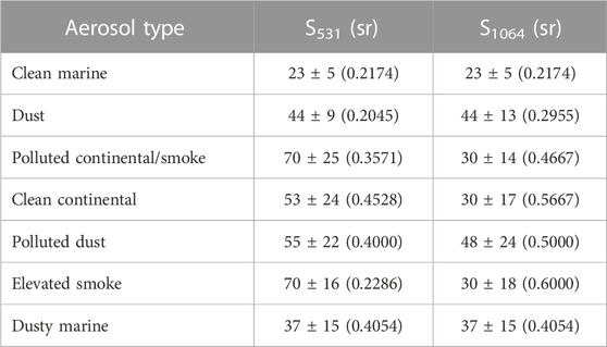
TABLE 1. Lidar ratios and absolute (relative) uncertainties for tropospheric aerosol types for CALIOP V4 aerosol retrievals (Kim et al., 2018).

In this paper, we first describe the ACTIVATE mission and the HSRL-2 instrument and measurements in Section 2. This section also describes the coincident and collocated airborne in situ measurements. The HSRL-2 observations of elevated depolarization for specific cases are presented in Section 3. Aerosol depolarization from non-spherical sea salt associated with changes in RH are discussed in this section, as are the HSRL-2 observations associated with these non-spherical aerosols throughout the ACTIVATE missions in 2020 and 2021. In Section 3 we also explain how these observations relate to the CALIOP measurements and show evidence of the CALIOP aerosol misclassification described above. Section 4 presents a summary of these observations and discusses possible ways to avoid such aerosol misclassification.

2 Methodology

2.1 ACTIVATE field mission

The measurements discussed here were acquired during the NASA EVS-3 ACTIVATE (Sorooshian et al., 2019). ACTIVATE’s overarching goal is to robustly characterize aerosol-cloud-meteorology interactions using extensive, systematic, and simultaneous in situ and remote sensing airborne measurements with two aircraft and a hierarchy of models (Sorooshian et al., 2019). ACTIVATE conducted 162 joint flights over the western Atlantic Ocean during a series of six deployments from 2020 to 2022. Here we use data collected during ACTIVATE winter and summer campaigns in 2020 and 2021 (Complete, final data from the 2022 deployment were unavailable at time of writing.) Joint flights were conducted using the NASA LaRC King Air, which flew at high altitude (∼9 km) and collected remote sensing and dropsonde data, and the NASA LaRC HU-25 Falcon, which simultaneously flew below the King Air at low altitude (0.3–2 km) and collected aerosol, cloud, trace gas, precipitation, and atmospheric state parameter measurements. Both aircraft were based at NASA Langley Research Center in Hampton, Virginia. The ACTIVATE measurements described here were acquired during the winter (February-March) and summer (August-September) flights in 2020 and during the winter (January-April) and summer (May-June) flights in 2021. All flights occurred during the daytime over the western Atlantic Ocean extending east several hundred kilometers from the coast and were typically about 3.5 h in duration. The majority (∼90%) of these flights were statistical survey flights. Brunke et al. (2022) and Dadashazar et al. (2022) provide descriptions of these flight patterns and maps showing flight locations.

2.2 NASA langley airborne high spectral resolution Lidar-2 (HSRL-2)

The second generation LaRC airborne HSRL instrument, HSRL-2, was deployed on the NASA Langley King Air aircraft during ACTIVATE. Similar to the LaRC’s first-generation HSRL, HSRL-1 (Hair et al., 2008), HSRL-2 uses the HSRL technique to independently retrieve aerosol and tenuous cloud extinction and backscatter (Shipley et al., 1983; Grund and Eloranta, 1991; She et al., 1992) without a priori assumptions on aerosol type and/or lidar ratio. HSRL-2 employs the HSRL technique at 355 and 532 nm and the standard elastic backscatter technique at 1,064 nm. It also measures aerosol and cloud depolarization at all three wavelengths. HSRL-2 employs an iodine cell to implement the HSRL technique at 532 nm and so HSRL-2 is essentially the same as HSRL-1 for measurements at 532 and 1,064 nm. HSRL measurements at 355 nm are made using an interferometer instead of an iodine cell (Burton et al., 2018).

When deployed on the King Air, HSRL-2 provides vertically resolved measurements of both aerosol extensive and intensive parameters below the aircraft. The aerosol extensive parameters include backscatter coefficient at 355, 532, and 1,064 nm (Δx ∼ 1 km, Δz ∼ 30 m); extinction coefficient via the HSRL technique at 355 and 532 nm (Δx ∼ 6 km, Δz ∼ 225 m); and optical depth at 355 and 532 nm (Approximate archival horizontal (Δx) and vertical resolutions (Δz) are listed in parentheses following each parameter.) The intensive parameters include extinction-to-backscatter ratio (S_a) at 355 and 532 nm (Δx ∼ 6 km, Δz ∼ 225 m); depolarization at 355, 532, and 1,064 nm (Δx ∼ 1 km, Δz ∼ 30 m); and aerosol backscatter wavelength dependence (i.e., Ǻngström exponent for aerosol backscatter, which is directly related to the backscatter color ratio) for two wavelength pairs (355–532 nm and 532–1,064 nm) (Δx ∼ 1 km, Δz ∼ 30 m). The profile measurements of aerosol backscatter are also used to derive aerosol mixed layer heights (MLH), which are associated with sharp gradients in the aerosol backscatter profiles (Scarino et al., 2013).

The HSRL-2 was designed so that it does not rely on an atmospheric target for calibration and so differs from standard elastic backscatter lidars, which must assume negligible or known aerosol amounts in the calibration region. The depolarization channels are calibrated using a rotating half-wave plate (Burton et al., 2015) and the aerosol and molecular measurements at 532 nm are determined using internal calibrations (Hair et al., 2008). The 1,064 nm backscatter coefficient measurement calibration constant and the 355 nm HSRL gain ratio between channels take advantage of the calibrated HSRL measurement at 532 nm in relatively clean regions of the flight. The overall systematic error associated with the backscatter calibration is estimated to be less than 2%–3%. Under typical conditions, the total systematic error for extinction coefficient is estimated to be less than 0.01 km⁻¹ at 532 nm. Rogers et al. (2009) validated the HSRL extinction coefficient profiles and found that the HSRL extinction profiles are within the typical state-of-the-art systematic error at visible wavelengths (Schmid et al., 2006). The random errors for all aerosol products are typically less than 10% for the backscatter and depolarization ratios (Hair et al., 2008). The systematic uncertainty in volume depolarization is estimated to be the larger of 4.7% (relative) or 0.001 (absolute) in the 355 nm channel, the larger of 5% (relative) or 0.007 (absolute) in the 532 nm channel, and the larger of 2.6% (relative) or 0.007 (absolute) in the 1,064 nm channel (Burton et al., 2015). The particulate (aerosol) depolarization ratio (see equation 2 in Burton et al. (2015)) depends on the total aerosol scattering ratio (i.e., ratio of aerosol to molecular scattering) as well as the volume depolarization ratio. Systematic uncertainties in particulate depolarization are typically less than 0.04 (355 nm) and 0.02 (532 and 1,064 nm) (Burton et al., 2015).

2.3 Airborne In situ measurements

Throughout ACTIVATE, profiles of water vapor, temperature, and winds were acquired by releasing Vaisala NRD412 “mini” dropsondes from the King Air using the Airborne Vertical Atmospheric Profiling System (AVAPS) dropsonde system (UCAR/NCAR, 1993; Hock and Franklin, 1999). Temperature and RH absolute uncertainties are ± 0.2°C and ± 3%, respectively (NCAR, 2022). Flight time when dropped from the King Air (∼9 km) is about 8–12 min. Typically, two to four dropsondes were released during each flight.

The NASA LaRC Falcon aircraft deployed in situ instruments to acquire measurements of aerosols, clouds, precipitation, and atmospheric state parameters while flying in a coordinated track below the King Air. An isokinetic aerosol inlet (Brechtel Manufacturing Inc.) was used to draw air into the aircraft cabin and allowed aerosols with aerodynamic diameters less than 5 μm to be sampled by cabin instruments. Submicrometer scattering and absorption coefficients were measured at three wavelengths by a nephelometer (TSI, Inc. Model 3563) and particle soot absorption photometer (PSAP, Radiance Research, Inc.), respectively. Aerosol dry size distributions between 3 and 100 nm (diameter) were measured by a TSI, Inc. Scanning Mobility particle Sizer (SMPS, Differential Mobility Analyzer model 3085) (Moore et al., 2017) and a TSI, Inc. Laser Aerosol Spectrometer (LAS) (model 3340) instrument measured dry aerosol size distributions between 100 and 5,000 nm (diameter) (Moore et al., 2021). The 5,000 nm cutoff in size was imposed by the sample inlet (McNaughton et al., 2007; Chen et al., 2011). The uncertainty in these size distribution measurements is better than ± 10–20% over the submicron size range (Moore et al., 2021). Submicrometer non-refractory aerosol chemical composition (sulfate, nitrate, ammonium, organics, and chlorine) was measured by a High-Resolution Time-of-Flight Aerosol Mass Spectrometer (HR-ToF-AMS) manufactured by Aerodyne Research (DeCarlo et al., 2006; Hilario et al., 2021). A particle-into-liquid sampler (PILS) instrument measured water-soluble concentrations of common ions using offline ion chromatography analysis (Sorooshian et al., 2006; Crosbie et al., 2020). A diode laser hygrometer (DLH) measured water vapor concentrations (Diskin et al., 2002). Temperature was measured by a Rosemount non-deiced total air temperature sensor (model E102E4AL) with a fast-response platinum sensing element (Thornhill et al., 2003). This sensor has a 20 m response time and an accuracy of 0.5 deg C. Regions where liquid water content was less than 0.001 gm⁻³ as derived from a cloud droplet probe (Droplet Measurement Technologies (Sinclair et al., 2019)) were classified as cloud-free (Schlosser et al., 2022).

3 Results

3.1 HSRL-2 observations of enhanced depolarization on 8 March 2020

HSRL-2 measurements over oceans typically show low (< 0.05) linear particulate depolarization at 532 nm because the aerosol is typically dominated by spherical sea salt, sulfate, and organic particles. For example, Figures 1A, B show HSRL-2 measurements of aerosol backscatter coefficient and particulate depolarization at 532 nm, respectively, for the ACTIVATE flights during the morning of 12 March 2020. These figures show profiles subsampled every 10 s (∼1 km). The flight track locations for the King Air and Falcon are shown in Figure 1C. Also shown in Figure 1B are color-coded RH values derived from the King Air dropsondes and the DLH measurements on board the Falcon. The Falcon in situ measurements were within 10 min and 20 km of the HSRL-2 measurements. Note the low (< 0.05) values of aerosol depolarization and the relatively high (>65%) RH values for most of the measurements below 1 km and extending downward to the surface. Particulate depolarization values at 355 and 1,064 nm (not shown) were also below 0.05. These low values of aerosol depolarization are consistent with the aerosol depolarization values typically reported for marine aerosols (Burton et al., 2012; Groß et al., 2013; Illingworth et al., 2015).

FIGURE 1

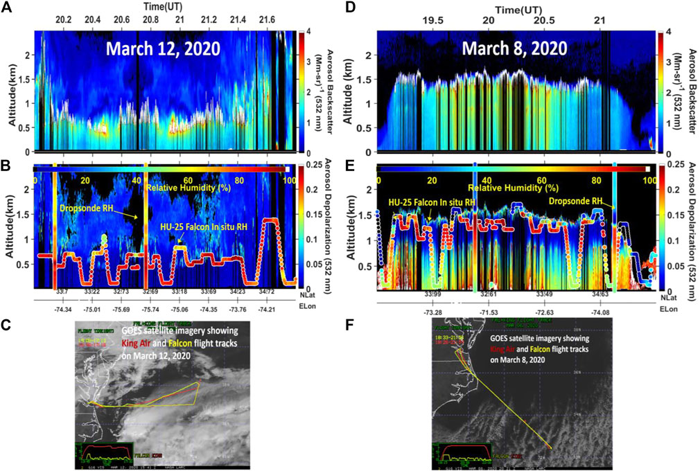
FIGURE 1. Profiles of (A) particulate backscatter and (B) particulate depolarization (532 nm) measured at 532 nm by HSRL-2 on 12 March 2020, with the corresponding color bars on the right. Also shown in (B) are in situ measurements of RH acquired from in situ measurements on the Falcon aircraft and dropsondes deployed from the King Air aircraft with the corresponding color bar at the top. Images are at 10 s (∼1 km) resolution. Cloudy areas are shown by the white areas in the backscatter images. Thick clouds completely attenuate the laser light leading to black stripes below these clouds. (C) Ground tracks of the King Air and Falcon aircraft are shown on GOES imagery. (D–F) show similar images of HSRL-2, airborne in situ, and dropsonde measurements and aircraft flight tracks for 8 March 2020. Note the pronounced increase in particulate depolarization on 8 March 2020.

In contrast, HSRL-2 measurements acquired during nearly a third of the flights conducted during 2020 and 2021 revealed enhanced particulate linear depolarization (>0.15–0.20 at 532 nm) associated with aerosols within the lowest several hundred meters of marine boundary layer. Figures 1D–F show one such example with aerosol backscatter, particulate depolarization profiles and flight track locations for the ACTIVATE flights on the afternoon of 8 March 2020. Also shown in Figures 1B, E are RH values derived from dropsonde and DLH measurements on the Falcon. Note the low RH (< 60%) values and high depolarization ratios (>0.15) occur within the lowest kilometer. High particulate depolarization values indicating the presence of non-spherical particles were also observed at 355 and 1,064 nm but are not shown. The highest depolarization values were found when the RH was below ∼60%.

Elevated depolarization measurements are commonly associated with lidar measurements of pollen (Sassen, 2008) or dust (Burton et al., 2015), but there is no evidence supporting significant amounts of dust or pollen in this 8 March 2020 case. NOAA Hybrid Single-Particle Lagrangian Integrated Trajectory (HYSPLIT) (Stein et al., 2015; Rolph et al., 2017) (https://www.ready.noaa.gov/HYSPLIT.php, last access: 30 March 2022) 3-day backtrajectories and FLEXible PARTicle dispersion model (FLEXPART) (https://www.flexpart.eu/, last access: 30 March 2022) (Stohl et al., 2005) 10-day back trajectories show air parcels in the lowest 2 km traveled from northern and western Canada and so it does not appear these observations of elevated depolarization were associated with Asian (Husar et al., 2001) or Saharan dust (Liu et al., 2008). Pollen has also been associated with lidar measurements of elevated depolarization (Bohlmann et al., 2021) but pollen and air quality reports over the mid-Atlantic states did not indicate high pollen levels (AirNow forecast from EnviroFlash http://www.cleanairpartners.net/).

GEOS-Chem (GC; http://www.geos-chem.org/) model simulations coincident with the HSRL-2 measurements were examined to gain insight into the aerosols producing such high particulate depolarization values. GC is a start-of-the-art 3-D chemical transport model. We use here the model version v11-01 (http://wiki.seas.harvard.edu/geos-chem/index.php/GEOS-Chem_v11-01, last access: November 2022) driven by meteorological fields from the MERRA-2 reanalysis from the NASA Global Modeling and Assimilation Office. The model resolution is 2 degrees latitude by 2.5 degrees longitude with 72 vertical levels. It includes sulfate-nitrate-ammonium thermodynamics coupled to ozone-NO_x-hydrocarbon-aerosol chemistry (Park et al., 2004), mineral dust in four size bins (Fairlie et al., 2007), sea salt in two size bins (Jaeglé et al., 2011), and elemental and organic carbon aerosols (Pye et al., 2010). Aerosol optical depths are calculated from the mass concentration, extinction efficiency, and particle mass density (Martin et al., 2003). Hourly model output values are sampled along the flight track. Figure 2A shows the HSRL-2 aerosol extinction (532 nm) “curtain” and Figure 2B shows the corresponding GC aerosol extinction (550 nm) “curtain” along the King Air flight track on 8 March 2020. Figures 2C–G show the contributions to the GC simulated aerosol extinction from various aerosol components. The GC total extinction values, which are in general agreement with the HSRL-2 measurements, are dominated by the contribution from sea salt aerosol (Figure 2F); aerosol extinction contributions by other aerosol components are negligible.

FIGURE 2

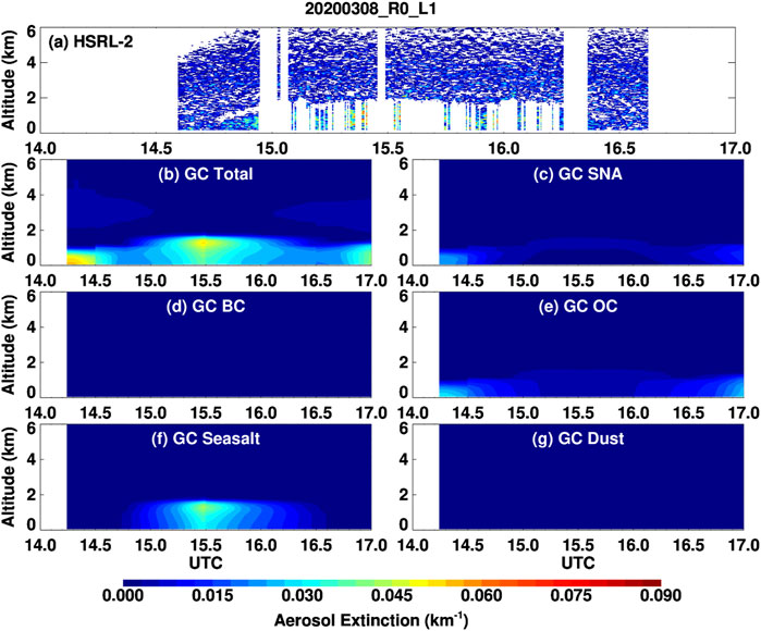
FIGURE 2. (A) Aerosol extinction derived from HSRL-2 measurements (532 nm) and (B) GEOS-Chem simulations (550 nm) of aerosol extinction during the 8 March 2020 morning flight. Aerosol extinction below and within clouds is not shown in the HSRL-2 results. Also shown are GEOS-Chem simulated contributions to aerosol extinction made by (C) sulfate + nitrate + ammonium, (D) black carbon, (E) organic carbon, (F) sea salt, and (G) dust. All panels share the same color bar. Note the large contribution to the GEOS-Chem aerosol extinction made by sea salt.

The HSRL-2 measurements of the lidar ratio showed average values for this day between 15 and 25 sr at both 355 and 532 nm below 1 km as shown in Figure 3. These values are considerably lower than the values derived from HSRL and Raman lidar measurements of dust (40–70 sr) and pollen (55–70) (Shang et al., 2020) and are consistent with sea salt (Müller et al., 2007; Burton et al., 2012; Groß et al., 2013).

FIGURE 3

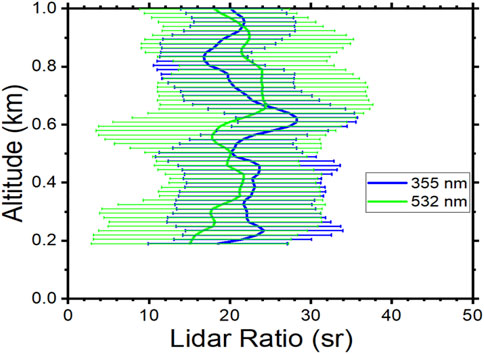
FIGURE 3. Average profiles of the lidar ratio derived from HSRL-2 observations at 355 and 532 nm during two flights (14:36–16:35 UT and 18:36–21:33 UT) on 8 March 2020. Error bars represent standard deviation of the measurements.

Figure 4 shows average profiles of water vapor mixing ratio and RH derived from the four dropsondes deployed during the morning and afternoon flights on 8 March 2020. The nearly constant mixing ratio suggests that the observations of elevated depolarization on this day occurred within a well-mixed boundary layer. The LAS airborne dry aerosol size distribution measurements acquired near the surface and at the top of the mixed layer were also very similar, which also supports that the HSRL-2 observations occurred within a well-mixed boundary layer (These size distribution measurements are discussed in more detail in Section 3.3.) Consequently, changes in aerosol intensive properties such as depolarization are due to changes in RH, and not due to changes in aerosol type.

FIGURE 4

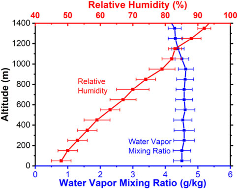
FIGURE 4. Average profiles of water vapor mixing ratio and relative humidity derived from the four dropsondes deployed during the flights on 8 March 2020. Each point represents the average of data from the four dropsondes and six altitudes averaged over 100 m deep layers. Error bars show the standard deviation of the measurements.

Figures 5A, B show expanded views of the HSRL-2 aerosol backscatter and depolarization measurements acquired between 19:45–20:00 UT on 8 March 2020. These figures show profiles sampled every 0.5 s (∼50 m). The pronounced increase in aerosol depolarization with decreasing RH is clearly shown in Figure 5B; Figures 5C,D show HSRL-2 aerosol backscatter and depolarization profiles along with the dropsonde RH profile at the time of the dropsonde at 19:52 UT. Note that while Figure 5C shows high (>0.1) depolarization at 532 nm generally below 1 km during this period, the depolarization varied below about 900 m. High values of aerosol depolarization are apparent as “plumes” with aerosol depolarization in excess of 0.2 separated by regions of lower (< 0.12) depolarization. These “plumes” of higher depolarization were separated by about 1.5–2 km. Based on the relationship between aerosol depolarization and RH, it appears that these plumes are likely plumes of dry (RH<60%) air separated by regions of moister air (RH>75%). Unfortunately, on this day, the Falcon did not fly level legs through these “plumes” (recall Figure 1E) to record these small-scale variations in RH. When RH exceeded about 75%–80% above about 900 m the aerosol depolarization dropped sharply to values below 0.05. The largest particulate depolarization values (>0.2) were generally located below 200–400 m where the RH was generally below about 50%–60%. Dropsonde wind speeds were less than 10 m/s within the lowest 1 km during these measurements.

FIGURE 5

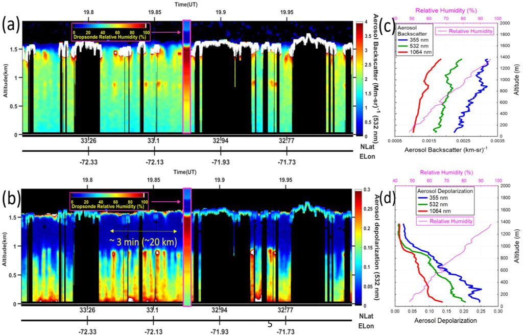
FIGURE 5. Expanded view of HSRL-2 profiles of (A) particulate backscatter (B) and particulate depolarization at 532 nm for the 8 March 2020 flight shown in Figure 1. Temporal resolution is 0.5 s (∼50 m). Also shown in these figures is the RH from the dropsonde at 19:52 UT with its corresponding color bar shown at the top. Cloudy areas are shown by the white areas in the backscatter images. Thick clouds completely attenuate the laser light leading to black stripes below these clouds. HSRL-2 multiwavelength profiles of (C) aerosol backscatter and (D) aerosol depolarization at the time of the dropsonde profile are also shown along with the dropsonde profile of RH.

3.2 Variability in sea salt depolarization due to relative humidity

We hypothesize these HSRL-2 observations of elevated and variable depolarization are associated with backscattering from sea salt particles whose shape varies with RH. Hygroscopic sea salt particles take on water with increasing RH and begin to deliquesce and eventually become spherical droplets as RH exceeds 70%–76% (Tang et al., 1997; Haarig et al., 2017; Zieger et al., 2017; Bi et al., 2018). This deliquescence point decreases slightly below 74% when salt particles are aggregated with other soluble particles (Wise et al., 2007). As the RH increases from 76% to 85%, the layer of water on the particles increases and the particles’ size rapidly increases. Above 85%, the water uptake continues, and the particles become essentially spherical. However, as revealed by x-ray phase contrast imaging, the actual deliquescence process of sea salt, which contains other species besides pure sodium-chloride, can also last over a much larger range of RH (34%–97%) compared to pure sodium-chloride (66%–89%) (Zeng et al., 2013). These images also revealed that, in such cases, sea salt did not encounter an abrupt deliquescence RH but rather remained a solid-liquid system at most of this RH range (Zeng et al., 2013).

In contrast, as RH decreases the particles retain their spherical shape and remain a droplet until the RH decreases below a threshold value of RH, when they start to lose water and solidify (efflorescence). This threshold value occurs around RH of ∼58% (Zeng et al., 2013; Haarig et al., 2017). The particles are then in a solid-liquid mix and the sea salt crystals grow as the RH continues to decrease to about 46% (Zeng et al., 2013). The hysteresis behavior described above means that, for RH between about 46% and 75%, sea salt can exist with both crystalline and spherical shapes depending on the history of the ambient RH.

The shape of the crystalline sea salt particles not only depends on their size and composition but also on the rate at which the particles have dried. Rapid drying rates cause rapid crystallization, which favor more spherical shapes; slower rates of drying lead to slower crystallization, which favor cubic shapes (Wang et al., 2010). At low RH (< 45%), crystalline sodium chloride has a cubic shape. However, dried sea salt particles are often but not always cubic (Bi et al., 2018); those that are cubic are not perfect cubes but rather have somewhat rounded edges (Haarig et al., 2017), which may be due to the chemical composition and the rate at which particles have dried. The addition of other compounds and sulfate can produce different geometries (Kandler et al., 2007; Wise et al., 2007); e.g., marine organics may produce a more spherical shape (Laskin et al., 2012).

This difference in how particle shape varies with increasing vs decreasing RH leads to corresponding differences in the behavior of particulate depolarization with changes in RH. Using a depolarization lidar, Haarig et al. (2017) observed changes in sea salt depolarization associated with both increasing and decreasing RH. With increasing RH, the particles keep their crystalline shape and produce higher depolarization, and then gradually become more spherical and produce smaller depolarization when RH increases above about 65%–70%. In contrast, with decreasing RH the particles maintain a spherical shape and low depolarization until the RH decreases to about 55%–60%, at which point the particles take on a cubic shape and the depolarization rapidly increases. Carrico et al. (2003) measured properties of aerosols including sea salt using humidified nephelometers on board the Ron Brown research vessel during ACE-Asia. Based on the behavior of scattering measurements made at various RH values, they found that the ambient aerosol was primarily on the upper (i.e., decreasing RH) branch of this hysteresis loop for marine aerosols. Murayama et al. (1999) reported on lidar depolarization measurements of particles near Tokyo Bay and found that the maximum depolarization occurred near RH of ∼66% rather than at lower RH; Bi et al. (2018) modeled the depolarization behavior of various particle shapes and particle size as a function of RH and suggested that this behavior reported by (Murayama et al., 1999) may be due to the water coating on the cubic particles, as their modeling found that the depolarization of coated cubes is larger than a bare cube.

Figure 6 shows mean particulate depolarization values at the three HSRL-2 wavelengths averaged over the dropsonde times during the 8 March 2020 flights as a function of the mean RH measured by these dropsondes. Similar results were obtained when examining HSRL-2 depolarization measurements coincident with the RH values derived from the DLH measurements on the Falcon aircraft. The curves show particulate depolarization was anti-correlated with RH. These results and those from Haarig et al. (2017) differ from the observations reported by Murayama et al. (1999) since there is no peak in the particulate depolarization values at 60%.

FIGURE 6

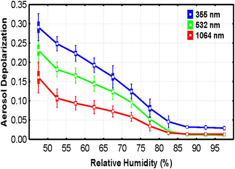
FIGURE 6. Box plot showing aerosol depolarization measured by HSRL-2 as a function of RH averaged over the four dropsonde times for the flights on 8 March 2020. Open squares show mean values, filled boxes show mean ± two standard errors, and whiskers show mean ± one standard deviation.

The vertical variability in the HSRL-2 aerosol depolarization measurements does not appear to be related to changes in the aerosol dry size distribution. The dry aerosol size distribution measured by the LAS on the Falcon aircraft near the top of the mixed layer was similar to the dry size distribution measured near the bottom of the mixed layer as shown in Figure 7A for the flights on 8 March 2020. On both March 8 and 12 March 2020 there was little vertical variability in the aerosol size distribution below 1 km. However, there was a significant change in the dry size distribution between these two dates. Figure 7B shows the dry size distribution for the 8 March 2020 afternoon flight when HSRL-2 measured enhanced depolarization and the dry size distribution for the morning flight on 12 March 2020 when HSRL-2 did not measure enhanced depolarization (recall Figure 1). During the flights on 8 March 2020, when HSRL-2 measured high aerosol depolarization, there were significantly fewer fine mode particles (i.e., particles with radii below 1 µm) than during the flights on 12 March 2020. Note the larger number of super micrometer size particles relative to the fine mode particles on 8 March 2020. The mean effective radius within the mixed layer decreased from 0.5 μm on 8 March 2020 to 0.3 μm on 12 March 2020. The relative lack of fine mode particles on 8 March 2020 likely led to coarse mode, non-spherical sea salt particles playing a larger role in contributing to the aerosol backscatter and extinction measured by HSRL-2.

FIGURE 7

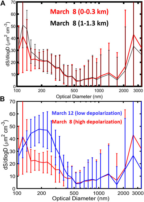
FIGURE 7. (A) Dry surface aerosol size distributions measured between 0 and 0.3 km and between 1 and 1.3 km by the Laser Aerosol Spectrometer (LAS) instrument on board the HU-25 Falcon on 8 March 2020 showing similar dry size distributions near the bottom and top of the marine boundary layer. (B) Dry surface aerosol size distributions measured between 0 and 0.3 km by the Laser Aerosol Spectrometer (LAS) instrument on board the HU-25 Falcon on 8 March 2020 (red) and 12 March 2020 (blue). Note the larger surface area associated with super micrometer particles relative to the fine mode particles on 8 March 2020 when HSRL-2 observed elevated depolarization. In contrast, the opposite occurred on 12 March 2020 when HSRL-2 observed low depolarization.

There have been various attempts to model the linear depolarization and lidar ratio of sea salt particles as they pertain to lidar measurements. However, modeling these optical properties is difficult and so such simulations have considerable uncertainties. As shown by Zeng et al. (2013), sea salt particles are often irregularly shaped so modeling their optical properties requires some simplifying assumptions about their shape(s). Various particle shapes (spheres, cubes, elongated and flattened cuboids, and superellipsoids resembling rounded cubes, spheres, and rounded octahedra) have been used to model the depolarization of sea salt particles (Bi et al., 2018; Kanngießer and Kahnert, 2021a; b). Modeling over realistic size distributions of irregularly shaped particles rather than single particles is often computationally not feasible especially when attempting to include particles in both fine and coarse modes (Kanngießer and Kahnert, 2021a). In addition, marine aerosols may contain various amounts of organic species leading to significant uncertainties in the modeled refractive index and the resulting modeled lidar ratio. Kanngieβer and Kahnert (2021a) found that the impacts of roundness and imaginary refractive index on linear depolarization are of similar magnitude.

Haarig et al. (2017) modeled depolarization and lidar ratios of dry, non-absorbing, cubic sea salt particles to explain the multiwavelength lidar measurements of depolarization and lidar ratios for sea salt aerosol over Barbados. They found general agreement between measured and modeled depolarization ratios when they assumed particle diameters were greater than the wavelength and some agreement with lidar ratios at 532 nm when they assumed particle diameters were greater than twice the wavelength. However, their modeled results overestimated linear depolarization at 1,064 nm and underestimated the lidar ratios at 355 nm. They attributed this to their modeled size distribution containing too many large particles. Kanngieβer and Kahnert (2021a) used superellipsoids comprised of cubes, rounded cubes, octahedra and rounded octahedra to model linear depolarization and lidar ratios of marine aerosols. Their simulations showed that the depolarization ratio varied between 0.14 and 0.20 and the lidar ratio varied between 12 and 20 sr for non-absorbing marine aerosols. Linear depolarization varied between 0.17 and 0.22 and lidar ratios varied between 25 and 33 sr for weakly absorbing aerosols. These results are consistent with the HSRL-2 observations reported here. Their simulations showed that both linear depolarization and lidar ratio varied significantly with refractive index so that refractive index is an important model tuning parameter and an important source of uncertainty. Depolarization produced by sea salt in various shapes coated by water has also been modeled by Bi et al. (2018). In general, the depolarization ratio of a coated cube is larger than a bare cube. These studies did not address the impacts of coating on lidar ratios. These previous studies suggest the HSRL-2 measurements of aerosol depolarization and lidar ratio values are best explained by diverse sea salt shapes, with variations in refractive indices associated with very weakly absorbing aerosols.

3.3 HSRL2 observations of elevated depolarization during ACTIVATE flights in 2020 and 2021

The HSRL-2 observations of elevated depolarization, such as those acquired on 8 March 2020, also occurred during numerous other ACTIVATE flights. During the ACTIVATE flights in 2020 and 2021, there were 63 days with coincident HSRL-2 and dropsonde measurements. Figure 8 shows the distribution of HSRL-2 aerosol depolarization measurements coincident with dropsonde RH measurements within the lowest 20% of the mixed layer (i.e., approximately the lowest 200–300 m) as defined by the HSRL-2 retrievals of mixed layer height (Scarino et al., 2013) on these 63 days. This altitude region is where the largest aerosol depolarization values were observed. Each point in this figure represents the average over all the dropsondes (∼4–8) on that date. HSRL-2 measurements of near-surface aerosol depolarization (532 nm) that exceeded 0.1 occurred simultaneously with dropsonde measurements of RH below 60% on 20 of the 63 days. These elevated depolarization observations occurred during 12 days in the winter (6 each in 2020 and 2021) and 8 days in spring/summer (3 in 2020 and 5 in 2021). Figure 8 shows that aerosol depolarization changes gradually from higher RH values until RH reaches ∼60% when there was a sharp transition in aerosol depolarization. Based on the hysteresis behavior illustrated by Haarig et al. (2017), this particular behavior shown in Figure 8 seems more consistent with sea salt particles retaining a more spherical shape as RH decreases until crystallization occurs around 60% as discussed above.

FIGURE 8

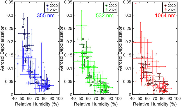
FIGURE 8. Dropsonde RH measurements and coincident HSRL-2 aerosol depolarization measurements at 355 nm (left), 532 nm (center), 1,064 nm (right) during 63 flight days conducted in 2020 and 2021. Each point represents the average over the lowest 20% of the mixed layer (i.e., approximately the lowest 200–300 m).

Figure 9 shows the average HSRL-2 depolarization as a function of dropsonde RH for all the HSRL-2/dropsonde coincidences during 2020 and 2021. These results are for altitudes z such that (z/Z_i<0.9) where Z_i is the MLH derived from the HSRL-2 data. The mean (standard deviation) MLH was 899 m (474 m). In addition, these coincidences are chosen such that water vapor mixing ratio was essentially constant through this altitude range, so changes in particle properties are assumed to be caused by changes in RH. Figure 9 shows a gradual decrease in aerosol depolarization with increasing RH when RH was less than about 75% like the 8 March 2020 case shown in Figure 6. Once RH increases above about 75%–85% there were smaller changes in aerosol depolarization as RH increased. Based on the hysteresis behavior illustrated by Haarig et al. (2017), this behavior, like that shown in Figure 6, is consistent with crystalline particles gradually taking on water as the RH increased until the particles reached the deliquescence point.

FIGURE 9

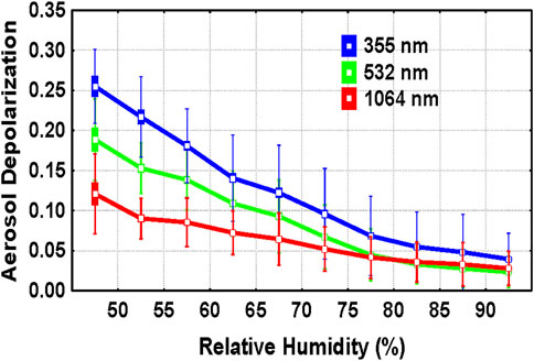
FIGURE 9. Box plot showing aerosol depolarization measured by HSRL-2 as a function of RH averaged over all the HSRL-2/dropsonde coincidences during 2020 and 2021. These results are for altitudes z such that (z/Z_i<0.9) where Z_i is the mixed layer height derived from the HSRL-2 data. Open squares show mean values, filled boxes show mean ± two standard errors, and whiskers show mean ± one standard deviation.

The average wavelength dependence is different from that reported by Haarig et al. (2017) who found the largest changes in aerosol depolarization associated with non-spherical sea salt occurred at 532 nm, with smaller increases in depolarization at 355 and 1,064 nm. As shown in Figures 6–9 the highest particulate depolarization values were above 0.25 at 355 nm, 0.2 at 532 nm, and 0.15 at 1,064 nm, which are considerably higher than the values measured in Haarig et al. (2017) (∼0.12, 0.15, 0.10 respectively). Based on field observations as well as laboratory experiments, linear depolarization ratios of up to 0.20–0.25 and lidar ratios of up to 25 sr can be considered plausible for dried sea salt aerosol (Kanngießer and Kahnert, 2021a). For the observations reported here, the largest increase in aerosol depolarization typically was measured at 355 nm and the smallest at 1,064 nm as shown in Figure 10. The difference in wavelength dependence may be due to different particle compositions in the different experiment locations; the measurements reported by Haarig et al. (2017) occurred over Barbados.

FIGURE 10

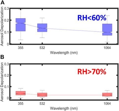
FIGURE 10. Median (line), 25–75 percentile (box), and 5–95 percentile (bars) aerosol depolarization values for (A) mean dropsonde RH< 60% in the lowest 300 m and (B) mean dropsonde RH>70% in the lowest 300 m derived from HSRL-2 and dropsonde data collected from 2020 to 2021.

The PILS and AMS composition measurements were used to estimate the contribution of sea salt to the dry aerosol mass. Sea salt mass was estimated as the sum of the PILS Na and Cl masses divided by an adjustment factor of 0.857 to account for other minor inorganic components (Seinfeld and Pandis, 1998), assuming the composition of sea-salt aerosol is equivalent to that of bulk seawater. The accumulation (fine) mode dry aerosol mass was estimated as the sum of the aerosol components measured by the AMS (i.e., Organics + SO4+NO3+NH4). Consequently, the sea salt mass fraction was computed as the ratio of the sea salt mass divided by the sum of the sea salt mass and accumulation mode dry mass. When elevated depolarization associated with non-spherical sea salt was observed on 8 March 2020, sea salt contributed about 80% to the total dry mass; in contrast, when low depolarization was observed on 12 March 2020, sea salt contributed about 40% of the total dry mass. The large fraction of sea salt present during the flights on 8 March 2020 likely accentuated the effects of RH on the aerosol depolarization associated with changes in sea salt shape. Some evidence of this can also be seen in Figure 11A, which shows that for RH below 60%, such as on 8 March 2020, aerosol depolarization tended to increase with increasing salt mass fraction. In contrast, for RH above 60%, when sea salt particles become more spherical and less crystalline, there was little correlation of aerosol depolarization with salt mass fraction.

FIGURE 11

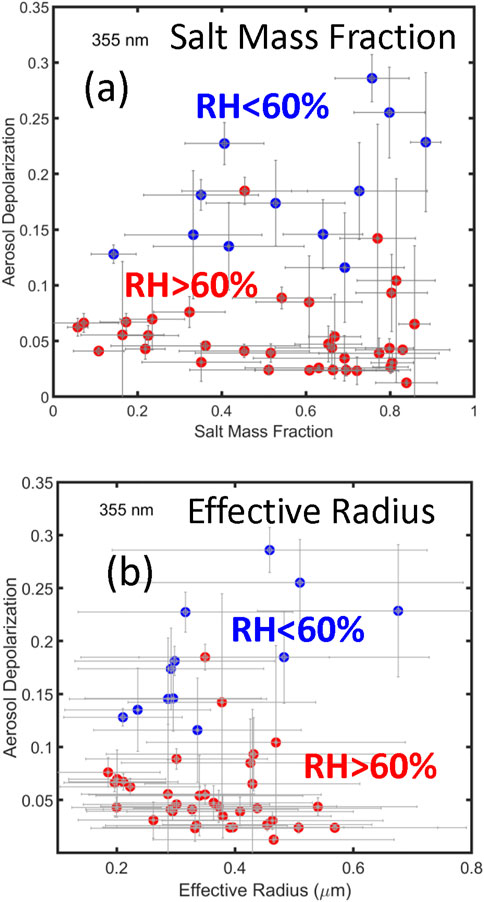
FIGURE 11. HSRL-2 measurements of aerosol depolarization at 355 nm vs. (A) salt mass fraction derived from the PILS and AMS measurements for RH< 60% (blue) and RH >60% (red) and (B) effective radii (dry) derived from the LAS measurements for RH< 60% (blue) and RH >60% (red). Each point represents the average of each flight and error bars represent the standard deviation over the flight. The Spearman rank correlation coefficients between aerosol depolarization and salt mass fraction are 0.66 (RH< 60%) and -0.16 (RH >60%). The Spearman rank correlation coefficients between aerosol depolarization and effective radius are 0.76 (RH< 60%) and -0.24 (RH >60%).

Effective radii corresponding to the dry aerosol were computed using the volume and surface concentrations measured by the LAS. Figure 11B shows that for RH below 60%, when the particles were more crystalline, the aerosol depolarization tended to increase with effective radius. For RH above 60%, when the particles were more spherical, there was little correlation between aerosol depolarization and effective radius. There was no correlation with the HSRL-2 measurements of aerosol depolarization with winds speeds measured by the dropsondes.

All the HSRL-2 profile observations throughout the ACTIVATE flights conducted in 2020 and 2021, not just those coincident with the dropsondes, were divided into two groups corresponding to whether the mean aerosol depolarization at 532 nm in the lowest 20% of the mixed layer was above or below 0.15. Figure 12A shows profiles of the aerosol depolarization for both groups. In the low depolarization group, the aerosol depolarization for each wavelength was generally at or below 0.05. In the high depolarization group, the aerosol depolarization increased with decreasing wavelength like the results in Figures 6, 8, 9. Figure 12B shows the aerosol extinction profiles associated with the low and high depolarization groups. Within the lowest kilometer, the aerosol extinction values associated with the high aerosol depolarization (i.e., non-spherical sea salt) group were about half those from the low depolarization group, with values generally less than 25 Mm⁻¹ at 532 nm. Based on the HSRL-2 observations these low values of aerosol extinction and high aerosol depolarization are associated with marine (sea salt) aerosols. The AOD contributed by these non-spherical particles was small (∼0.03–0.04 at 532 nm). In contrast, the higher values of aerosol extinction and low values of aerosol depolarization often correspond to the presence of other aerosols. Figure 12C shows the lidar ratio profiles associated with the two aerosol depolarization groups. As expected, the lidar ratios (355 and 532 nm) within the lowest 1.5 km associated with the high aerosol depolarization group are around 20–25 sr, which corresponds to marine (sea salt) aerosols. The lidar ratios associated with the low aerosol depolarization cases are generally higher as these cases may include other aerosol types such as urban aerosol and or biomass burning smoke, which have higher lidar ratios (recall Table 1). Figure 12D shows the lidar ratio vs aerosol depolarization throughout the mixed layer for the high depolarization group and, like Figures 12A, C, shows that the lidar ratios at both 355 and 532 nm were essentially constant even though aerosol depolarization varied between about 0.5 and 0.2.

FIGURE 12

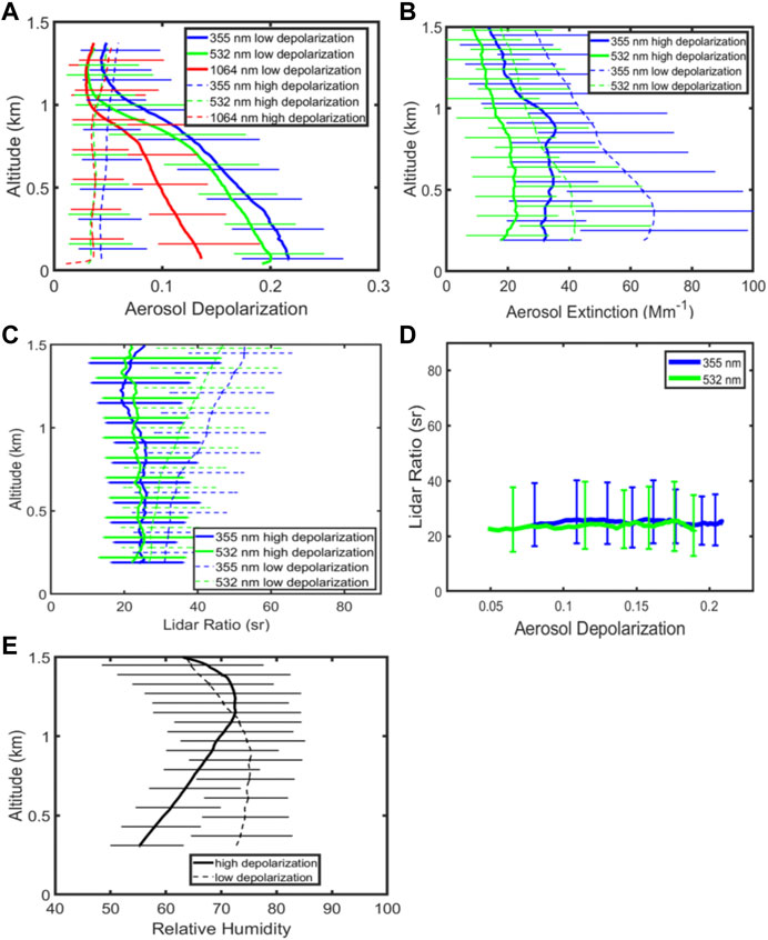
FIGURE 12. HSRL-2 profiles of (A) aerosol depolarization at 355, 532, and 1,064 nm, (B) aerosol extinction at 355 and 532 nm, and (C) lidar ratio at 355, and 532 nm for cases of low and high depolarization within the lowest 20% of the mixed layer using data from all flights. Low depolarization cases were chosen such that the median aerosol depolarization at 532 nm in the lowest 20% of the mixed layer was less than 0.15 for a given flight; high depolarization cases were chosen such that the median aerosol depolarization at 532 nm in the lowest 20% of the mixed layer was greater than 0.15 for a given flight. (D) Lidar ratio vs. aerosol depolarization throughout the mixed layer for the subset of high depolarization cases shown in a-c. (E) MERRA-2 profiles of RH for these same low and high depolarization cases.

Figure 12E shows profiles of RH corresponding to these two aerosol depolarization groups. These are RH profiles provided by the MERRA-2 reanalysis (Bosilovich et al., 2016) at three hourly intervals and 0.5 ° × 0.625 ° horizontal resolution interpolated to the King Air flight track location and HSRL-2 measurement times. A comparison of the MERRA-2 and dropsonde RH profiles shows that the MERRA-2-derived RH values were, on average, within 3% of the dropsonde-derived RH values for RH below 80% but become progressively drier by 5%–10% once the dropsonde RH exceeds 90%. These results are consistent with those reported by Seethala et al. (2021). The RH profile associated with the low depolarization group is generally above 70% within the lowest kilometer, which is consistent with the relationships between aerosol depolarization and RH discussed earlier. These results suggest that the MERRA-2 RH profiles may provide some guidance in locating regions where non-spherical aerosols may (or may not) be present. Above 1.5 km (not shown in Figure 12D), the RH associated with the high depolarization cases was generally below 20% in contrast to the high depolarization cases when RH was generally higher than 40%. This suggests that entrainment of dry air into the marine boundary layer may be associated with the observations of low RH and high depolarization.

3.4 Implications for CALIOP aerosol retrievals

The CALIOP instrument on board the Cloud Aerosol Lidar and Infrared Pathfinder Satellite Observation (CALIPSO) satellite provides retrievals of aerosol backscatter and extinction profiles at 532 and 1,064 nm and profiles of particle depolarization at 532 nm (Winker et al., 2009). Unlike HSRLs, which directly measure range-resolved particulate scattering ratios, CALIOP measures total attenuated backscatter, which is the product of the total backscatter coefficient at a particular range bin and the total two-way transmittance (i.e., signal attenuation) between the lidar and that range bin. The total backscatter coefficient is the sum of the particulate and molecular contributions. Similarly, the total two-way transmittance is the combined signal attenuation due to all molecules and particulates along the path between the lidar and the measurement location. To retrieve particulate backscatter and extinction coefficients from the CALIOP measurements, layer-mean lidar ratios must be specified for each particulate type encountered within a profile (Young, 1995; Omar et al., 2009; Young and Vaughan, 2009). On those relatively infrequent occasions when independent layer optical depth estimates are available, layer-mean lidar ratios can be derived directly from the CALIOP attenuated backscatter signals. When an independent constraint is not available, the current CALIOP algorithms use lookup tables that prescribe lidar ratios for a predetermined set of aerosol types, as shown in Table 1. The accuracies of the CALIOP aerosol extinction and backscatter profiles thus depend on the representativeness of these aerosol lidar ratios, as well as on the ability to accurately infer the appropriate aerosol type from the CALIOP measurements (Rogers et al., 2014).

The CALIOP algorithm uses the integrated attenuated backscatter at 532 nm, estimated particulate depolarization ratio, aerosol layer altitude, and measurement location to identify the aerosol type and subsequently select the lidar ratio (Omar et al., 2009). The presence of non-spherical sea salt particles with elevated (>0.15) depolarization values and low lidar ratios (20–25 sr) has important implications for CALIOP inferences of aerosol type and lidar ratios and subsequent retrievals of AOD and aerosol extinction profiles. Currently, when CALIOP detects elevated (>0.075) estimated particulate depolarization, the aerosol is classified as dusty marine, polluted dust or desert dust depending on the magnitude of the estimated particulate depolarization, layer altitude and location. These aerosol types have lidar ratios considerably larger than clean marine, as shown in Table 1. Consequently, the misclassification of sea salt as dust or a dust mixture leads to large (>60%) relative biases in CALIOP retrievals of AOD and aerosol extinction profiles.

Figure 13 shows a likely example of such a CALIOP misclassification that occurred on 9 March 2020, about 12 h after and in the same region as the HSRL-2 observations shown in Figures 1D,E. The CALIOP level 1 attenuated backscatter measurements in Figure 13A show an aerosol layer below about 1 km. The CALIOP level 2 integrated attenuated backscatter measurements shown in Figure 13B are dominated by this aerosol layer. The CALIOP retrievals of integrated particulate depolarization ratio in Figure 13C show elevated depolarization north of about 34.33 deg N (approximately the left half of the graph). Based on these elevated (>0.08) integrated particulate depolarization ratios, the integrated attenuated backscatter values, the over-ocean location, and low (< 2.5 km) layer altitude, the CALIOP algorithm classified these aerosols as dusty marine with a corresponding lidar ratio of 37 sr (Figure 13D). South of about 34.33 N (approximately the right half of the graph), the lower (< 0.08) integrated particulate depolarization ratios led to the classification of the aerosol layer below 1.5 km as clean marine with a corresponding lidar ratio of 23 sr. The MERRA-2 RH profiles shown in Figure 13E have lower values (< 65%) in the region of higher depolarization and conversely higher (>65%) values in the region of lower depolarization suggesting that sea salt is likely to be the primary contributor to observed particulate depolarization variability. GEOS-Chem model simulations driven by MERRA-2 (not shown) indicate that sea salt had the largest contribution to aerosol extinction within the lowest layer over the region at this time, further suggesting that the CALIOP algorithm misclassified the sea salt as dusty marine. The impact of this change in aerosol classification on the derived AOD is shown in Figure 13F. The probable misclassification of the clean marine aerosol in the left half of the graph leads to AOD values about 0.01–0.02 (about 40%–80%) higher than AOD values computed assuming the aerosols were clean marine.

FIGURE 13

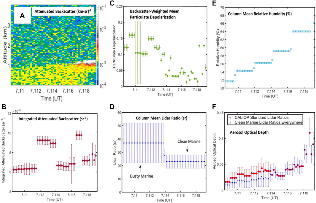
FIGURE 13. CALIOP (A) level 1 profiles of attenuated backscatter at 532 nm, (B) level 2 profiles of integrated attenuated backscatter at 532 nm, (C) backscatter-weighted mean integrated particulate depolarization ratio at 532 nm, (D) column mean lidar ratio at 532 nm, (E) column mean RH from MERRA-2 model, and (F) tropospheric aerosol optical depth at 532 nm derived from the CALIOP data using the standard lidar ratios (red) and lidar ratios corresponding to clean marine aerosol (blue). All panels correspond to the period 07:06–07:14 UT on 9 March 2020 when CALIOP acquired data in the region of the aircraft flights shown in Figure 1F.

This CALIOP misclassification may occur relatively often during specific types of meteorological events. The elevated depolarization associated with sea salt observed in the HSRL-2 measurements during ACTIVATE tended to occur during maritime cold air outbreaks (CAO), which are equatorward excursions of cold polar air masses over the relatively warm open ocean (Painemal et al., 2021; Terpstra et al., 2021; Corral et al., 2022). Several of the ACTIVATE flights conducted during 2020 and 2021 occurred during CAOs (Seethala et al., 2021). CALIOP observations of total attenuated backscatter (532 nm), particulate depolarization ratio (532 nm), and aerosol subtype along with MERRA-2 and ERA5 assimilated fields of RH and temperature profiles and surface wind speeds during 15 CAO events in January-March 2019 were examined to estimate the frequency of such observations. Each of these 15 events included some aerosol that the CALIOP algorithm classified as dusty marine. In 12 of these events, the location of the measurements, the absence of elevated aerosol layers suggesting little higher-level dust transport from the continent, and the assimilated data sets showing low (< 70%) RH near the surface within a well-mixed boundary layer suggest that the CALIOP operational algorithm misclassified depolarizing sea salt as dusty marine aerosol. Such misclassifications could lead to some systematic high biases in the retrievals of AOD and aerosol extinction profiles. Given the HSRL-2 measurements of relatively low AOD and aerosol extinction associated with these non-spherical sea salt observations (recall Figure 12B) and the CALIOP example shown in Figure 13F, the absolute biases in aerosol extinction and layer AOD would be relatively small (< 0.02), but the relative biases would be large (∼50%).

Li et al. (2022) assessed CALIOP V4.2 aerosol types and assigned lidar ratios (recall Table 1) using AOD retrievals from the Synergized Optical Depth of Aerosols (SODA) algorithm (Josset et al., 2008; Josset et al., 2011) and the retrieved columnar lidar ratio estimated by combining SODA AOD and CALIOP attenuated backscatter. Using CALIOP data acquired over the ocean from 2006 to 2011, they found that the V4.2 assigned lidar ratios and the lidar ratios derived using the SODA AOD constraint were in good agreement for clean marine aerosol over the open ocean, elevated smoke over the southeast Atlantic Ocean, and dust over the subtropical Atlantic Ocean. However, they found that over the open ocean, for aerosols classified as dusty marine aerosol (S_a = 37), the lidar ratios retrieved using the SODA AOD columnar constraint had magnitudes and spatial distributions like those classified as clean marine (S_a = 23). Their conclusion that some dusty marine aerosols should be classified as clean marine support the observations reported here of the presence of depolarizing sea salt.

4 Summary and conclusion

Lidar measurements typically show low (< 0.05 at 532 nm) linear particulate depolarization associated with marine sea salt aerosols (Burton et al., 2012; Groß et al., 2013; Illingworth et al., 2015). However, during 20 of the 63 days in 2020 and 2021 when the NASA ACTIVATE mission conducted flights over the western Atlantic Ocean, airborne HSRL-2 and dropsonde measurements revealed that elevated depolarization (>0.1 at 532 nm) occurred within marine boundary layers within several hundred meters to a kilometer above the surface. These observations of elevated depolarization typically occurred during cold air outbreaks when the RH at these altitudes is below about 60%. The strong correlation of elevated depolarization with low (< 60%) RH, low aerosol lidar ratios (20–25 sr) at 532 nm and 355 nm, coincident airborne in situ size and composition measurements, and aerosol transport models indicate that the elevated depolarization is associated with crystalline sea salt. These observations of elevated depolarization occurred during both winter and summer. Largest values of particulate depolarization occurred at 355 nm (∼0.25–0.30), in contrast to results reported by Haarig et al. (2017) who found the largest values at 532 nm. The aerosol extinction and optical thickness corresponding to these non-spherical sea salt particles were low; aerosol extinction values were around 20 Mm⁻¹ at 532 nm and the optical depth contributed by these non-spherical particles was about 0.03–0.04 at 532 nm which represented on average about 30%–40% of the total column AOD. These HSRL-2 multiwavelength measurements of aerosol depolarization and lidar ratio are examples of the type of field measurements that can be used to help refine models of the optical properties of marine aerosols under different meteorological conditions (Kahnert and Kanngießer, 2023).

Airborne in situ measurements of aerosol size distribution and fine mode aerosol composition acquired simultaneously with the HSRL-2 measurements revealed that the elevated depolarization measurements occurred when more coarse mode particles relative to fine mode particles were observed in contrast to observations of lower depolarization when more fine mode particles were observed. In those cases when RH was below 60%, aerosol depolarization was correlated with both salt mass fraction and particle effective radius but was not correlated with wind speed.

The presence of non-spherical sea salt can lead to possible misidentification of these aerosols as a dust-like mixture. The CALIOP operational aerosol classification algorithm classifies aerosols, including non-spherical sea salt, as various mixtures of dust when aerosol depolarization is above about 0.075. This misclassification of non-spherical sea salt leads to a high bias in the lidar ratio assigned to these aerosols, which in turn leads to high biases in the aerosol extinction and AOD derived from the CALIOP measurements. Examination of CALIOP measurements during several CAO episodes and SODA retrievals of column lidar ratio suggest that the CALIOP operational aerosol algorithm tended to classify these non-spherical aerosols as dusty marine rather than marine aerosols during CAO events.

How can such misclassification of sea salt be avoided? Examination of model (e.g., MERRA-2) reanalysis RH profiles coincident with the ACTIVATE dropsonde and HSRL-2 measurements indicates that such profiles may provide an indication of the low RH conditions leading to the presence of non-spherical sea salt. While the presence of low (< 60%) RH by itself does not necessarily indicate the presence of such aerosols since other non-spherical aerosols (e.g., dust) may also be associated with low RH, the spatial and vertical variability in RH, when well correlated with similar variability in aerosol depolarization, would likely provide a good indicator of non-spherical sea salt. In addition, the presence of higher (>70%) RH would essentially rule out the presence of non-spherical sea salt.

The wavelength dependence of depolarization may help discriminate between non-spherical sea salt and dust, especially if depolarization is measured at both 355 and 532 nm. The HSRL-2 measurements showed aerosol depolarization was generally larger at 355 nm than at 532 nm, in contrast to aerosol depolarization measurements of dust where aerosol depolarization at 532 nm is larger (Burton et al., 2015). The spectral depolarization between 532 and 1,064 nm is less definitive. Burton et al. (2012) found that dust depolarization at 1,064 nm could be lower, higher, or about the same as the value at 532 nm. Since the HSRL-2 measurements of sea salt showed smaller aerosol depolarization at 1,064 nm than at 532 nm, the presence of higher aerosol depolarization at 1,064 nm would likely indicate the presence of dust and not non-spherical sea salt.

Measurements of the lidar ratio provide a more definitive discrimination between dust and non-spherical sea salt. Non-spherical sea salt had similar lidar ratio values as spherical sea salt (∼20–25 sr at both 355 and 532 nm) that are lower than the values typically measured for dust (e.g., 30–50 sr) (Burton et al., 2012). For backscatter lidars such as CALIOP on CALIPSO, which do not measure the lidar ratio directly, the total column AOD may be a useful constraint to derive a lidar ratio associated with the depolarizing aerosols for cases where most, if not all, of the total AOD is due to these depolarizing aerosols and these layers have well-defined boundaries and large optical depths. This column AOD constraint can be provided by AOD retrieved from passive sensors during the daytime (e.g., MODIS (Burton et al., 2010)) or from techniques such that use the ocean surface reflectance to derive column transmission and AOD (Josset et al., 2008; Venkata and Reagan, 2016). More direct measurements of the lidar ratio associated with the depolarizing aerosols by a spaceborne High Spectral Resolution Lidar such as the ATLID lidar on the EarthCARE satellite could also help distinguish non-spherical sea salt and dust.

Data availability statement

Publicly available datasets were analyzed in this study. This data can be found here:

HSRL-2 and other data from the NASA ACTIVATE mission are available from https://asdc.larc.nasa.gov/project/ACTIVATE. CALIPSO data are available via Langley Research Center’s Atmospheric Science Data Center (ASDC) at https://asdc.larc.nasa.gov/project/CALIPSO. The GEOS-Chem model code is available at http://wiki.seas.harvard.edu/geos-chem/index.php/GEOS-Chem_v11-01.

Author contributions

Data analyses: RF, MF, MC, AS, and SC. Data providers: JH, CH, TS, DH, SS, AC, EC, EW, LZ, LT, CR, RM, MV, AS, HL, BZ, GD, JD, JN, and YC, Text: all authors. All authors contributed to the article and approved the submitted version.

Funding

This work was funded through the NASA ACTIVATE Earth Venture Suborbital-3 (EVS-3) investigation, which is funded by the NASA Earth Science Division and managed through the Earth System Science Pathfinder Program Office. AS was partially supported by ONR grant N00014-21-1-2115. JS was supported by appointment to the NASA Postdoctoral Program at NASA Langley Research Center, administered by Oak Ridge Associated Universities under contract with NASA. HL and BZ were supported by NASA grant 80NSSC19K038.

Acknowledgments

We thank pilots, aircrew, and maintenance personnel from the NASA Langley Research Center Research Services Division for their dedicated support in conducting the extensive ACTIVATE flights. The satellite images were obtained from the NASA LaRC Satellite ClOud and Radiation Property retrieval System (SatCORPS) Team, https://satcorps.larc.nasa.gov. The authors gratefully acknowledge the NOAA Air Resources Laboratory for the HYSPLIT transport and dispersion model and the READY website (http://ready.arl.noaa.gov). HL and BZ would like to thank the GEOS-Chem support team at Harvard University and Washington University in St. Louis for their effort. The NASA Center for Climate Simulation (NCCS) provided supercomputing resources for the GEOS-Chem simulation.

Conflict of interest

Authors MF, MC, AS, EC, EW, LT, CR, and YC were employed by the company Science Systems and Applications, Inc.

The remaining authors declare that the research was conducted in the absence of any commercial or financial relationships that could be construed as a potential conflict of interest.

Publisher’s note

All claims expressed in this article are solely those of the authors and do not necessarily represent those of their affiliated organizations, or those of the publisher, the editors and the reviewers. Any product that may be evaluated in this article, or claim that may be made by its manufacturer, is not guaranteed or endorsed by the publisher.

References

Anderson, T. L., Charlson, R. J., Winker, D. M., Ogren, J. A., and Holmen, K. (2003). Mesoscale variations of tropospheric aerosols. J. Atmos. Sci. 60 (1), 119–136. doi:10.1175/1520-0469(2003)060<0119:mvota>2.0.co;2

CrossRef Full Text | Google Scholar

Bi, L., Lin, W., Wang, Z., Tang, X., Zhang, X., and Yi, B. (2018). Optical modeling of sea salt aerosols: The effects of nonsphericity and inhomogeneity. J. Geophys. Res. Atmos. 123 (1), 543–558. doi:10.1002/2017jd027869

CrossRef Full Text | Google Scholar

Bohlmann, S., Shang, X., Vakkari, V., Giannakaki, E., Leskinen, A., Lehtinen, K. E., et al. (2021). Lidar depolarization ratio of atmospheric pollen at multiple wavelengths. Atmos. Chem. Phys. 21 (9), 7083–7097. doi:10.5194/acp-21-7083-2021

CrossRef Full Text | Google Scholar

Bosilovich, M. G., Lucchesi, R., and Suarez, M. (2016). MERRA-2: File specification. GMAO Office Note No. 9. Version 1.1.

Google Scholar

Brunke, M. A., Cutler, L., Urzua, R. D., Corral, A. F., Crosbie, E., Hair, J., et al. (2022). Aircraft observations of turbulence in cloudy and cloud-free boundary layers over the western north Atlantic Ocean from ACTIVATE and implications for the Earth system model evaluation and development. J. Geophys. Res. Atmos. 127 (19), e2022JD036480. doi:10.1029/2022JD036480

CrossRef Full Text | Google Scholar

Burton, S., Hair, J., Kahnert, M., Ferrare, R., Hostetler, C., Cook, A., et al. (2015). Observations of the spectral dependence of linear particle depolarization ratio of aerosols using NASA Langley airborne High Spectral Resolution Lidar. Atmos. Chem. Phys. 15 (23), 13453–13473. doi:10.5194/acp-15-13453-2015

CrossRef Full Text | Google Scholar

Burton, S., Hostetler, C., Cook, A., Hair, J., Seaman, S., Scola, S., et al. (2018). Calibration of a high spectral resolution lidar using a Michelson interferometer, with data examples from ORACLES. Appl. Opt. 57 (21), 6061–6075. doi:10.1364/ao.57.006061

PubMed Abstract | CrossRef Full Text | Google Scholar

Burton, S. P., Ferrare, R. A., Hostetler, C. A., Hair, J. W., Kittaka, C., Vaughan, M. A., et al. (2010). Using airborne high spectral resolution lidar data to evaluate combined active plus passive retrievals of aerosol extinction profiles. J. Geophys. Research-Atmospheres 115, D00H15. doi:10.1029/2009jd012130

CrossRef Full Text | Google Scholar

Burton, S. P., Ferrare, R. A., Hostetler, C. A., Hair, J. W., Rogers, R. R., Obland, M. D., et al. (2012). Aerosol classification of airborne high spectral resolution lidar measurements – methodology and examples. Atmos. Meas. Tech. 5, 73–98. doi:10.5194/amt-5-73-2012

CrossRef Full Text | Google Scholar

Carrico, C. M., Kus, P., Rood, M. J., Quinn, P. K., and Bates, T. S. (2003). Mixtures of pollution, dust, sea salt, and volcanic aerosol during ACE-Asia: Radiative properties as a function of relative humidity. J. Geophys. Res. 108 (23), 8650. doi:10.1029/2003jd003405

CrossRef Full Text | Google Scholar

Chen, G., Ziemba, L. D., Chu, D. A., Thornhill, K. L., Schuster, G. L., Winstead, E. L., et al. (2011). Observations of Saharan dust microphysical and optical properties from the Eastern Atlantic during NAMMA airborne field campaign. Atmos. Chem. Phys. 11 (2), 723–740. doi:10.5194/acp-11-723-2011

CrossRef Full Text | Google Scholar

Corral, A. F., Choi, Y., Crosbie, E., Dadashazar, H., DiGangi, J. P., Diskin, G. S., et al. (2022). Cold air outbreaks promote new particle formation off the U.S. East coast. Geophys. Res. Lett. 49 (5), e2021GL096073. doi:10.1029/2021GL096073

CrossRef Full Text | Google Scholar

Crosbie, E., Shook, M. A., Ziemba, L. D., Anderson, B. E., Braun, R. A., Brown, M. D., et al. (2020). Coupling an online ion conductivity measurement with the particle-into-liquid sampler: Evaluation and modeling using laboratory and field aerosol data. Aerosol Sci. Technol. 54 (12), 1542–1555. doi:10.1080/02786826.2020.1795499

PubMed Abstract | CrossRef Full Text | Google Scholar

Dadashazar, H., Crosbie, E., Choi, Y., Corral, A. F., DiGangi, J. P., Diskin, G. S., et al. (2022). Analysis of MONARC and ACTIVATE airborne aerosol data for aerosol-cloud interaction investigations: Efficacy of stairstepping flight legs for airborne in situ sampling. Atmosphere 13 (8), 1242. doi:10.3390/atmos13081242

CrossRef Full Text | Google Scholar

DeCarlo, P. F., Kimmel, J. R., Trimborn, A., Northway, M. J., Jayne, J. T., Aiken, A. C., et al. (2006). Field-deployable, high-resolution, time-of-flight aerosol mass spectrometer. Anal. Chem. 78 (24), 8281–8289. doi:10.1021/ac061249n

PubMed Abstract | CrossRef Full Text | Google Scholar

Diskin, G. S., Podolske, J. R., Sachse, G. W., and Slate, T. A. (2002). “Open-path airborne tunable diode laser hygrometer,” in Diode lasers and applications in atmospheric sensing: SPIE), 196–204.

CrossRef Full Text | Google Scholar

Fairlie, T. D., Jacob, D. J., and Park, R. J. (2007). The impact of transpacific transport of mineral dust in the United States. Atmos. Environ. 41 (6), 1251–1266. doi:10.1016/j.atmosenv.2006.09.048

CrossRef Full Text | Google Scholar

Groß, S., Esselborn, M., Weinzierl, B., Wirth, M., Fix, A., and Petzold, A. (2013). Aerosol classification by airborne high spectral resolution lidar observations. Atmos. Chem. Phys. 13, 2487–2505. doi:10.5194/acp-13-2487-2013

CrossRef Full Text | Google Scholar

Grund, C. J., and Eloranta, E. W. (1991). University-of-Wisconsin high spectral resolution lidar. Opt. Eng. 30 (1), 6–12. doi:10.1117/12.55766

CrossRef Full Text | Google Scholar

Haarig, M., Ansmann, A., Gasteiger, J., Kandler, K., Althausen, D., Baars, H., et al. (2017). Dry versus wet marine particle optical properties: RH dependence of depolarization ratio, backscatter, and extinction from multiwavelength lidar measurements during SALTRACE. Atmos. Chem. Phys. 17 (23), 14199–14217. doi:10.5194/acp-17-14199-2017

CrossRef Full Text | Google Scholar

Hair, J. W., Hostetler, C. A., Cook, A. L., Harper, D. B., Ferrare, R. A., Mack, T. L., et al. (2008). Airborne high spectral resolution lidar for profiling aerosol optical properties. Appl. Opt. 47 (36), 6734. doi:10.1364/ao.47.006734

PubMed Abstract | CrossRef Full Text | Google Scholar

Hilario, M. R. A., Crosbie, E., Shook, M., Reid, J. S., Cambaliza, M. O. L., Simpas, J. B. B., et al. (2021). Measurement report: Long-range transport patterns into the tropical northwest pacific during the CAMP&amp;lt;sup&amp;gt;2&amp;lt;/sup&amp;gt;Ex aircraft campaign: Chemical composition, size distributions, and the impact of convection. Atmos. Chem. Phys. 21 (5), 3777–3802. doi:10.5194/acp-21-3777-2021

CrossRef Full Text | Google Scholar

Hock, T. F., and Franklin, J. L. (1999). The ncar gps dropwindsonde. Bull. Am. Meteorological Soc. 80 (3), 407–420. doi:10.1175/1520-0477(1999)080<0407:tngd>2.0.co;2

CrossRef Full Text | Google Scholar

Husar, R. B., Tratt, D., Schichtel, B. A., Falke, S., Li, F., Jaffe, D., et al. (2001). Asian dust events of April 1998. J. Geophys. Res. Atmos. 106 (D16), 18317–18330. doi:10.1029/2000jd900788

CrossRef Full Text | Google Scholar

Illingworth, A. J., Barker, H., Beljaars, A., Ceccaldi, M., Chepfer, H., Clerbaux, N., et al. (2015). The EarthCARE satellite: The next step forward in global measurements of clouds, aerosols, precipitation, and radiation. Bull. Am. Meteorological Soc. 96 (8), 1311–1332. doi:10.1175/bams-d-12-00227.1

CrossRef Full Text | Google Scholar

Jaeglé, L., Quinn, P., Bates, T., Alexander, B., and Lin, J.-T. (2011). Global distribution of sea salt aerosols: New constraints from in situ and remote sensing observations. Atmos. Chem. Phys. 11 (7), 3137–3157. doi:10.5194/acp-11-3137-2011

CrossRef Full Text | Google Scholar

Josset, D., Pelon, J., Protat, A., and Flamant, C. (2008). New approach to determine aerosol optical depth from combined CALIPSO and CloudSat ocean surface echoes. Geophys. Res. Lett. 35 (10). doi:10.1029/2008gl033442

CrossRef Full Text | Google Scholar

Josset, D., Rogers, R., Pelon, J., Hu, Y., Liu, Z., Omar, A., et al. (2011). CALIPSO lidar ratio retrieval over the ocean. Opt. Express 19 (19), 18696–18706. doi:10.1364/oe.19.018696

PubMed Abstract | CrossRef Full Text | Google Scholar

Kahnert, M., and Kanngießer, F. (2023). Optical properties of marine aerosol: Modelling the transition from dry, irregularly shaped crystals to brine-coated, dissolving salt particles. J. Quantitative Spectrosc. Radiat. Transf. 295, 108408. doi:10.1016/j.jqsrt.2022.108408

CrossRef Full Text | Google Scholar

Kandler, K., Benker, N., Bundke, U., Cuevas, E., Ebert, M., Knippertz, P., et al. (2007). Chemical composition and complex refractive index of Saharan Mineral Dust at Izaña, Tenerife (Spain) derived by electron microscopy. Atmos. Environ. 41 (37), 8058–8074. doi:10.1016/j.atmosenv.2007.06.047

CrossRef Full Text | Google Scholar

Kanngießer, F., and Kahnert, M. (2021a). Modeling optical properties of non-cubical sea-salt particles. J. Geophys. Res. Atmos. 126 (4), e2020JD033674.

Google Scholar

Kanngießer, F., and Kahnert, M. (2021b). Optical properties of water-coated sea salt model particles. Opt. Express 29 (22), 34926–34950. doi:10.1364/oe.437680

PubMed Abstract | CrossRef Full Text | Google Scholar

Kim, M.-H., Omar, A. H., Tackett, J. L., Vaughan, M. A., Winker, D. M., Trepte, C. R., et al. (2018). The CALIPSO version 4 automated aerosol classification and lidar ratio selection algorithm. Atmos. Meas. Tech. 11 (11), 6107–6135. doi:10.5194/amt-11-6107-2018

PubMed Abstract | CrossRef Full Text | Google Scholar

Laskin, A., Moffet, R. C., Gilles, M. K., Fast, J. D., Zaveri, R. A., Wang, B., et al. (2012). Tropospheric chemistry of internally mixed sea salt and organic particles: Surprising reactivity of NaCl with weak organic acids. J. Geophys. Res. Atmos. 117 (D15). doi:10.1029/2012jd017743

CrossRef Full Text | Google Scholar

Lewis, E. R., and Schwartz, S. E. (2004). sea salt aerosol production: Mechanisms, methods, measurements, and models. American Geophysical Union.

Google Scholar

Li, Z., Painemal, D., Schuster, G., Clayton, M., Ferrare, R., Vaughan, M., et al. (2022). Assessment of tropospheric CALIPSO Version 4.2 aerosol types over the ocean using independent CALIPSO–SODA lidar ratios. Atmos. Meas. Tech. 15 (9), 2745–2766. doi:10.5194/amt-15-2745-2022

CrossRef Full Text | Google Scholar

Liu, Z. Y., Omar, A., Vaughan, M., Hair, J., Kittaka, C., Hu, Y. X., et al. (2008). CALIPSO lidar observations of the optical properties of saharan dust: A case study of long-range transport. J. Geophys. Research-Atmospheres 113, D07207. doi:10.1029/2007jd008878

CrossRef Full Text | Google Scholar

Martin, R. V., Jacob, D. J., Yantosca, R. M., Chin, M., and Ginoux, P. (2003). Global and regional decreases in tropospheric oxidants from photochemical effects of aerosols. J. Geophys. Res. Atmos. 108 (D3). doi:10.1029/2002JD002622

CrossRef Full Text | Google Scholar

McNaughton, C. S., Clarke, A. D., Howell, S. G., Pinkerton, M., Anderson, B., Thornhill, L., et al. (2007). Results from the DC-8 inlet characterization experiment (DICE): Airborne versus surface sampling of mineral dust and sea salt aerosols. Aerosol Sci. Technol. 41 (2), 136–159. doi:10.1080/02786820601118406

CrossRef Full Text | Google Scholar

Moore, R. H., Thornhill, K. L., Weinzierl, B., Sauer, D., D’Ascoli, E., Kim, J., et al. (2017). Biofuel blending reduces particle emissions from aircraft engines at cruise conditions. Nature 543 (7645), 411–415. doi:10.1038/nature21420

PubMed Abstract | CrossRef Full Text | Google Scholar

Moore, R. H., Wiggins, E. B., Ahern, A. T., Zimmerman, S., Montgomery, L., Campuzano Jost, P., et al. (2021). Sizing response of the ultra-high sensitivity aerosol spectrometer (UHSAS) and laser aerosol spectrometer (LAS) to changes in submicron aerosol composition and refractive index. Atmos. Meas. Tech. 14 (6), 4517–4542. doi:10.5194/amt-14-4517-2021

CrossRef Full Text | Google Scholar

Müller, D., Mattis, I., Ansmann, A., Wandinger, U., Ritter, C., and Kaiser, D. (2007). Multiwavelength Raman lidar observations of particle growth during long-range transport of forest-fire smoke in the free troposphere. Geophys. Res. Lett. 34 (5). doi:10.1029/2006GL027936

CrossRef Full Text | Google Scholar

Murayama, T., Furushima, M., Oda, A., Iwasaka, N., and Kai, K. (1996). Depolarization ratio measurements in the atmospheric boundary layer by lidar in Tokyo. J. Meteorological Soc. Jpn. 74 (4), 571–578. doi:10.2151/jmsj1965.74.4_571

CrossRef Full Text | Google Scholar

Murayama, T., Okamoto, H., Kaneyasu, N., Kamataki, H., and Miura, K. (1999). Application of lidar depolarization measurement in the atmospheric boundary layer: Effects of dust and sea-salt particles. J. Geophys. Research-Atmospheres 104 (D24), 31781–31792. doi:10.1029/1999jd900503

CrossRef Full Text | Google Scholar

NCAR (2022). AVAPS dropsondes. Accessed June 2022.

Google Scholar

Omar, A. H., Winker, D. M., Kittaka, C., Vaughan, M. A., Liu, Z. Y., Hu, Y. X., et al. (2009). The CALIPSO automated aerosol classification and lidar ratio selection algorithm. J. Atmos. Ocean. Technol. 26 (10), 1994–2014. doi:10.1175/2009JTECHA1231.1

CrossRef Full Text | Google Scholar

Painemal, D., Corral, A. F., Sorooshian, A., Brunke, M. A., Chellappan, S., Afzali Gorooh, V., et al. (2021). An overview of atmospheric features over the western north Atlantic Ocean and north American east coast—Part 2: Circulation, boundary layer, and clouds. J. Geophys. Res. Atmos. 126 (6), e2020JD033423. doi:10.1029/2020JD033423

CrossRef Full Text | Google Scholar

Park, R. J., Jacob, D. J., Field, B. D., Yantosca, R. M., and Chin, M. (2004). Natural and transboundary pollution influences on sulfate-nitrate-ammonium aerosols in the United States: Implications for policy. J. Geophys. Res. Atmos. 109 (D15), D15204. doi:10.1029/2003jd004473

CrossRef Full Text | Google Scholar

Pye, H., Chan, A., Barkley, M., and Seinfeld, J. (2010). Global modeling of organic aerosol: The importance of reactive nitrogen (NO&amp;lt;sub&amp;gt;x&amp;lt;/sub&amp;gt; and NO&amp;lt;sub&amp;gt;3&amp;lt;/sub&amp;gt;). Atmos. Chem. Phys. 10 (22), 11261–11276. doi:10.5194/acp-10-11261-2010

CrossRef Full Text | Google Scholar

Rogers, R. R., Hair, J. W., Hostetler, C. A., Ferrare, R. A., Obland, M. D., Cook, A. L., et al. (2009). NASA LaRC airborne high spectral resolution lidar aerosol measurements during MILAGRO: Observations and validation. Atmos. Chem. Phys. 9 (14), 4811–4826. doi:10.5194/acp-9-4811-2009

CrossRef Full Text | Google Scholar

Rogers, R., Vaughan, M., Hostetler, C., Burton, S., Ferrare, R., Young, S., et al. (2014). Looking through the haze: Evaluating the CALIPSO level 2 aerosol optical depth using airborne high spectral resolution lidar data. Atmos. Meas. Tech. 7 (12), 4317–4340. doi:10.5194/amt-7-4317-2014

CrossRef Full Text | Google Scholar

Rolph, G., Stein, A., and Stunder, B. (2017). Real-time environmental applications and display system: Ready. Environ. Model. Softw. 95, 210–228. doi:10.1016/j.envsoft.2017.06.025

CrossRef Full Text | Google Scholar

Sakai, T., Shibata, T., Kwon, S.-A., Kim, Y.-S., Tamura, K., and Iwasaka, Y. (2000). Free tropospheric aerosol backscatter, depolarization ratio, and relative humidity measured with the Raman lidar at nagoya in 1994–1997: Contributions of aerosols from the asian continent and the pacific ocean. Atmos. Environ. 34 (3), 431–442. doi:10.1016/s1352-2310(99)00328-3

CrossRef Full Text | Google Scholar

Sassen, K. (2008). Boreal tree pollen sensed by polarization lidar: Depolarizing biogenic chaff. Geophys. Res. Lett. 35 (18), L18810. doi:10.1029/2008gl035085

CrossRef Full Text | Google Scholar

Sassen, K. (1977). Ice crystal habit discrimination with the optical backscatter depolarization technique. J. Appl. Meteorology 16 (4), 425–431. doi:10.1175/1520-0450(1977)016<0425:ichdwt>2.0.co;2

CrossRef Full Text | Google Scholar

Sassen, K. (2000). “Lidar backscatter depolarization technique for cloud and aerosol research,” in Light scattering by nonspherical particles: Theory, measurements, and applications. Editors M. I. Mishchenko, J. W. Hovenier, and L. D. Travis (San Diego, CA: Academic).

CrossRef Full Text | Google Scholar

Scarino, A. J., Obland, M. D., Fast, J. D., Burton, S. P., Ferrare, R. A., Hostetler, C. A., et al. (2013). Comparison of mixed layer heights from airborne high spectral resolution lidar, ground-based measurements, and the WRF-Chem model during CalNex and CARES. Atmos. Chem. Phys. Discuss. 13 (5), 13721–13772. doi:10.5194/acpd-13-13721-2013

CrossRef Full Text | Google Scholar

Schlosser, J. S., Stamnes, S., Burton, S. P., Cairns, B., Crosbie, E., Van Diedenhoven, B., et al. (2022). Polarimeter + lidar–derived aerosol particle number concentration. Front. Remote Sens. 3. doi:10.3389/frsen.2022.885332

CrossRef Full Text | Google Scholar

Schmid, B., Ferrare, R., Flynn, C., Elleman, R., Covert, D., Strawa, A., et al. (2006). How well do state-of-the-art techniques measuring the vertical profile of tropospheric aerosol extinction compare? J. Geophys. Res. 111, D05S07. doi:10.1029/2005jd005837

CrossRef Full Text | Google Scholar

Schuster, G. L., Vaughan, M., MacDonnell, D., Su, W., Winker, D., Dubovik, O., et al. (2012). Comparison of CALIPSO aerosol optical depth retrievals to AERONET measurements, and a climatology for the lidar ratio of dust. Atmos. Chem. Phys. 12 (16), 7431–7452. doi:10.5194/acp-12-7431-2012

CrossRef Full Text | Google Scholar

Seethala, C., Zuidema, P., Edson, J., Brunke, M., Chen, G., Li, X. Y., et al. (2021). On assessing ERA5 and MERRA2 representations of cold-air outbreaks across the Gulf Stream. Geophys. Res. Lett. 48 (19), e2021GL094364. doi:10.1029/2021gl094364

PubMed Abstract | CrossRef Full Text | Google Scholar

Seinfeld, J. H., and Pandis, S. N. (1998). From air pollution to climate change. Atmos. Chem. Phys. 1326.

Google Scholar

Shang, X., Giannakaki, E., Bohlmann, S., Filioglou, M., Saarto, A., Ruuskanen, A., et al. (2020). Optical characterization of pure pollen types using a multi-wavelength Raman polarization lidar. Atmos. Chem. Phys. 20 (23), 15323–15339. doi:10.5194/acp-20-15323-2020

CrossRef Full Text | Google Scholar

She, C. Y., Alvarez, R. J., Caldwell, L. M., and Krueger, D. A. (1992). High-spectral-resolution Rayleigh-mie lidar measurement of aerosol and atmospheric profiles. Opt. Lett. 17 (7), 541–543. doi:10.1364/ol.17.000541

PubMed Abstract | CrossRef Full Text | Google Scholar

Shipley, S. T., Tracy, D. H., Eloranta, E. W., Trauger, J. T., Sroga, J. T., Roesler, F. L., et al. (1983). High spectral resolution lidar to measure optical-scattering properties of atmospheric aerosols .1. Theory and instrumentation. Appl. Opt. 22 (23), 3716–3724. doi:10.1364/ao.22.003716

PubMed Abstract | CrossRef Full Text | Google Scholar

Sinclair, K., Van Diedenhoven, B., Cairns, B., Alexandrov, M., Moore, R., Crosbie, E., et al. (2019). Polarimetric retrievals of cloud droplet number concentrations. Remote Sens. Environ. 228, 227–240. doi:10.1016/j.rse.2019.04.008

CrossRef Full Text | Google Scholar

Sorooshian, A., Anderson, B., Bauer, S. E., Braun, R. A., Cairns, B., Crosbie, E., et al. (2019). Aerosol–cloud–meteorology interaction airborne field investigations: Using lessons learned from the US West coast in the design of activate off the US East Coast. Bull. Am. Meteorological Soc. 100 (8), 1511–1528. doi:10.1175/bams-d-18-0100.1

CrossRef Full Text | Google Scholar

Sorooshian, A., Brechtel, F. J., Ma, Y., Weber, R. J., Corless, A., Flagan, R. C., et al. (2006). Modeling and characterization of a particle-into-liquid sampler (PILS). Aerosol Sci. Technol. 40 (6), 396–409. doi:10.1080/02786820600632282

CrossRef Full Text | Google Scholar

Stein, A. F., Draxler, R. R., Rolph, G. D., Stunder, B. J. B., Cohen, M. D., and Ngan, F. (2015). NOAA’s HYSPLIT atmospheric transport and dispersion modeling system. Bull. Am. Meteorological Soc. 96 (12), 2059–2077. doi:10.1175/bams-d-14-00110.1

CrossRef Full Text | Google Scholar

Stohl, A., Forster, C., Frank, A., Seibert, P., and Wotawa, G. (2005). Technical note: The Lagrangian particle dispersion model FLEXPART version 6.2. Atmos. Chem. Phys. 5 (9), 2461–2474. doi:10.5194/acp-5-2461-2005

CrossRef Full Text | Google Scholar

Sugimoto, N., Matsui, I., Shimizu, A., Pinandito, M., and Sugondo, S. (2000). Climatological characteristics of cloud distribution and planetary boundary layer structure in Jakarta, Indonesia revealed by lidar observation. Geophys. Res. Lett. 27 (18), 2909–2912. doi:10.1029/2000gl011544

CrossRef Full Text | Google Scholar

Tang, I. N., Tridico, A., and Fung, K. (1997). Thermodynamic and optical properties of sea salt aerosols. J. Geophys. Res. Atmos. 102 (D19), 23269–23275. doi:10.1029/97jd01806

CrossRef Full Text | Google Scholar

Terpstra, A., Renfrew, I. A., and Sergeev, D. E. (2021). Characteristics of cold-air outbreak events and associated polar mesoscale cyclogenesis over the North Atlantic region. J. Clim. 34 (11), 1–52. doi:10.1175/jcli-d-20-0595.1

CrossRef Full Text | Google Scholar

Thornhill, K. L., Anderson, B. E., Barrick, J. D., Bagwell, D. R., Friesen, R., and Lenschow, D. H. (2003). Air motion intercomparison flights during transport and chemical evolution in the pacific (trace-P)/ACE-ASIA. J. Geophys. Res. Atmos. 108 (D20), 9001. doi:10.1029/2002jd003108

CrossRef Full Text | Google Scholar

UCAR/NCAR (1993). “Earth observing laboratory,” in NCAR airborne vertical atmospheric profiling system (AVAPS) (UCAR/NCAR - Earth Observing Laboratory). Retrieved December 2021. doi:10.5065/D66W9848

CrossRef Full Text | Google Scholar

Vaughan, M., Pitts, M., Trepte, C., Winker, D., Detweiler, P., Garnier, A., et al. (2019). Cloud-Aerosol LIDAR Infrared Pathfinder Satellite Observations (CALIPSO) data management system data products catalog. NASA Langley Research Center Document.

Google Scholar

Venkata, S. L., and Reagan, J. A. (2016). Aerosol retrievals from CALIPSO lidar ocean surface returns. Remote Sens. 8 (12), 1006. doi:10.3390/rs8121006

CrossRef Full Text | Google Scholar

Wang, Z., King, S. M., Freney, E., Rosenoern, T., Smith, M. L., Chen, Q., et al. (2010). The dynamic shape factor of sodium chloride nanoparticles as regulated by drying rate. Aerosol Sci. Technol. 44 (11), 939–953. doi:10.1080/02786826.2010.503204

CrossRef Full Text | Google Scholar

Winker, D. M., Vaughan, M. A., Omar, A., Hu, Y. X., Powell, K. A., Liu, Z. Y., et al. (2009). Overview of the CALIPSO mission and CALIOP data processing algorithms. J. Atmos. Ocean. Technol. 26 (11), 2310–2323. doi:10.1175/2009jtecha1281.1

CrossRef Full Text | Google Scholar

Wise, M. E., Semeniuk, T. A., Bruintjes, R., Martin, S. T., Russell, L. M., and Buseck, P. R. (2007). Hygroscopic behavior of NaCl-bearing natural aerosol particles using environmental transmission electron microscopy. J. Geophys. Res. Atmos. 112 (D10). doi:10.1029/2006jd007678

CrossRef Full Text | Google Scholar

Young, S. A. (1995). Analysis of lidar backscatter profiles in optically thin clouds. Appl. Opt. 34 (30), 7019–7031. doi:10.1364/ao.34.007019

PubMed Abstract | CrossRef Full Text | Google Scholar

Young, S. A., and Vaughan, M. A. (2009). The retrieval of profiles of particulate extinction from cloud-aerosol lidar infrared pathfinder satellite observations (CALIPSO) data: Algorithm description. J. Atmos. Ocean. Technol. 26 (6), 1105–1119. doi:10.1175/2008JTECHA1221.1

CrossRef Full Text | Google Scholar

Zeng, J., Zhang, G., Long, S., Liu, K., Cao, L., Bao, L., et al. (2013). sea salt deliquescence and crystallization in atmosphere: An in situ investigation using x-ray phase contrast imaging. Surf. interface analysis 45 (5), 930–936. doi:10.1002/sia.5184

CrossRef Full Text | Google Scholar

Zieger, P., Väisänen, O., Corbin, J. C., Partridge, D. G., Bastelberger, S., Mousavi-Fard, M., et al. (2017). Revising the hygroscopicity of inorganic sea salt particles. Nat. Commun. 8 (1), 15883–15910. doi:10.1038/ncomms15883

PubMed Abstract | CrossRef Full Text | Google Scholar