Accuracy and Reproducibility of Above-Water Radiometry With Calibrated Smartphone Cameras Using RAW Data

Consumer cameras, especially on smartphones, are popular and effective instruments for above-water radiometry. The remote sensing reflectance R_rs is measured above the water surface and used to estimate inherent optical properties and constituent concentrations. Two smartphone apps, HydroColor and EyeOnWater, are used worldwide by professional and citizen scientists alike. However, consumer camera data have problems with accuracy and reproducibility between cameras, with systematic differences of up to 40% in intercomparisons. These problems stem from the need, until recently, to use JPEG data. Lossless data, in the RAW format, and calibrations of the spectral and radiometric response of consumer cameras can now be used to significantly improve the data quality. Here, we apply these methods to above-water radiometry. The resulting accuracy in R_rs is around 10% in the red, green, and blue (RGB) bands and 2% in the RGB band ratios, similar to professional instruments and up to 9 times better than existing smartphone-based methods. Data from different smartphones are reproducible to within measurement uncertainties, which are on the percent level. The primary sources of uncertainty are environmental factors and sensor noise. We conclude that using RAW data, smartphones and other consumer cameras are complementary to professional instruments in terms of data quality. We offer practical recommendations for using consumer cameras in professional and citizen science.

1 Introduction

The remote sensing reflectance R_rs(λ) is an apparent optical property that contains a wealth of information about the substances within the water column (IOCCG, 2008). In above-water radiometry, R_rs is measured using one or more (spectro)radiometers deployed above the water surface (Ruddick et al., 2019). The absorption and scattering coefficients and concentrations of colored dissolved organic matter (CDOM), suspended particulate matter, and prominent phytoplankton pigments such as chlorophyll-a (chl-a) can be determined from R_rs (Werdell et al., 2018). Due to spectral range and long-term stability requirements, the equipment necessary for accurate measurements of R_rs is often expensive. High costs limit the uptake and, therefore, impact of these instruments.

Consumer cameras have long been seen as a low-cost alternative or complement to professional instruments (Sunamura and Horikawa, 1978). Work in this direction has mostly focused on hand-held digital cameras, which measure the incoming radiance in red-green-blue (RGB) spectral bands typically spanning the visible range from 390 to 700 nm (Goddijn-Murphy et al., 2009). Uncrewed aerial vehicles (UAVs or drones) and webcams have similar optical properties, often contain the same sensors, and are also increasingly used in remote sensing (Burggraaff et al., 2019). Consumer cameras have been used to retrieve CDOM, chl-a, and suspended mineral concentrations through above-water radiometry (Goddijn-Murphy et al., 2009; Hoguane et al., 2012). They are particularly useful for measuring at small spatial scales, short cadence, and over long time periods (Lim et al., 2010; Iwaki et al., 2021).

Smartphones are especially effective as low-cost sensing platforms thanks to their wide availability, cameras, and functionalities including accelerometers, GPS, and wireless communications. They are already commonly used in place of professional sensors in laboratories (Friedrichs et al., 2017; Hatiboruah et al., 2020). However, what smartphones truly excel at is providing a platform for citizen science in the field (Snik et al., 2014; Garcia-Soto et al., 2021). There is a vibrant ecosystem of applications (apps) using the smartphone camera for environmental citizen science purposes (Andrachuk et al., 2019). Some use additional fore-optics to measure hyperspectrally (Burggraaff et al., 2020; Stuart et al., 2021), while most use the camera as it is (Busch J. et al., 2016; Leeuw and Boss, 2018; Gao et al., 2022). Smartphone science apps are also commonly used for educational purposes and in professional research (Gallagher and Chuan, 2018; Ayeni and Odume, 2020; Al-Ghifari et al., 2021).

Two apps are currently widely used for above-water radiometry, namely HydroColor (Leeuw and Boss, 2018) and EyeOnWater (Busch J. et al., 2016). HydroColor measures R_rs in the RGB bands using the Mobley (1999) protocol, guiding the user to the correct pointing angles with on-screen prompts. Through an empirical algorithm based on the red band of R_rs, the app estimates the turbidity, suspended matter concentration, and backscattering coefficient of the target body of water. EyeOnWater uses the WACODI algorithm (Novoa et al., 2015) to determine the hue angle α of the water, representing its intrinsic color. From α it also estimates the Forel-Ule (FU) index, a discrete water color scale with a century-long history (Novoa et al., 2013). α and the FU index are reasonable first-order indicators of the surface chl-a concentration and optical depth (Pitarch et al., 2019).

While these apps and other consumer camera-based methods provide useful data, improvements to the accuracy and reproducibility are necessary to derive high-quality end products. Validation campaigns have consistently found the radiance, R_rs in the RGB bands, and hue angle from consumer cameras to be well-correlated with reference instruments, but often with a wide dispersion and a significant bias. For R_rs, the mean difference between smartphone and reference match-up data is typically $\ge 0.003$ sr⁻¹ or $\ge 30\%$, but varies wildly between studies (Leeuw and Boss, 2018; Yang et al., 2018; Gao et al., 2020, 2022). As an extreme example, Malthus et al. (2020) found no correlation at all between HydroColor and reference R_rs data, albeit under challenging observing conditions. The typical accuracy in α is around 10° or 1–2 FU (Novoa et al., 2015; Busch J. A. et al., 2016; Malthus et al., 2020; Gao et al., 2022). Differences in R_rs between smartphones can be as large as 40% (Yang et al., 2018). The uncertainties, as well as the differences between smartphones and reference instruments, in observed optical properties and derived water constituent concentrations are often even greater than 40% (Ouma et al., 2018; Malthus et al., 2020; Pratama et al., 2021), although this may be explained in part by differences in inherent optical properties and observing conditions between study sites.

A major source of uncertainty in existing methods is the use of the JPEG data format. Until recently JPEG was the only format available to third-party developers on most smartphones and other consumer cameras. JPEG data are irreversibly compressed and post-processed for visual appeal, at the cost of radiometric accuracy and dynamic range. Most importantly, they are very nonlinear, meaning a 2× increase in radiance does not cause a 2× increase in response (Burggraaff et al., 2019). Instead, in a process termed gamma correction or gamma compression, the radiance is scaled by a power law. The nonlinearity of JPEG data is a significant contributor to the uncertainty in R_rs obtained from consumer cameras and apps such as HydroColor (Burggraaff et al., 2019; Gao et al., 2020; Malthus et al., 2020). Some approaches, including WACODI, attempt to correct for nonlinearity through an inverse gamma correction (Novoa et al., 2015; Gao et al., 2020). This inverse correction cannot be performed consistently because the smartphone JPEG processing differs between smartphone brands, models, and firmware versions (Burggraaff et al., 2019).

A secondary source of uncertainty are the spectral response functions (SRFs) of the cameras. Because exact SRF profiles are laborious to measure and are rarely provided by manufacturers, it is often necessary to use simplified SRFs and assume them to be device-independent (Novoa et al., 2015; Leeuw and Boss, 2018). However, the SRFs of different cameras actually vary significantly (Burggraaff et al., 2019).

The quality of consumer camera radiometry can be improved significantly by using lossless data, in the RAW format, and camera calibrations. RAW data are almost entirely unprocessed and thus are not affected by the uncertainties introduced by the JPEG format. Furthermore, through calibration and characterization of the radiometric and spectral response, consumer cameras can be used as professional-grade (spectro)-radiometers (Burggraaff et al., 2019).

In this work, we assess the uncertainty, reproducibility, and accuracy of calibrated smartphone cameras, using RAW data, for above-water radiometry. By comparing in situ observations from two smartphone cameras and two hyperspectral instruments, we test the hypothesis that the new methods decrease the uncertainty and increase the reproducibility and accuracy of data from consumer cameras. To our knowledge, this is the first time that the new methods have been applied or assessed in a field setting.

Section 2 describes the data acquisition and processing as well as the performed experiments. The results are presented in Section 3. In Section 4, we discuss the results, compare them to the literature, and present some recommendations for projects using smartphones. Finally, the conclusions of the analysis are presented in Section 5.

2 Methods

Smartphone and reference data were gathered on and around Lake Balaton, Hungary, from 3 to 5 July 2019. Lake Balaton is the largest (597 km²) lake in central Europe, with a mean depth of only 3.3 m, and is well-studied. It has a high concentration of suspended mineral particles and appears very bright and turquoise (bluish-green) to the eye (Figure 1, further discussed in Section 2.1). Due to inflow from the Zala river, the western side of the lake is richer in nutrients than the eastern side. The adjacent Kis-Balaton reservoir is hypereutrophic with chl-a concentrations up to 160 mg m⁻³. More detailed descriptions of this site are given in Riddick (2016) and Palmer (2015).

FIGURE 1

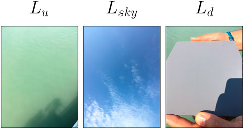
FIGURE 1. Example iPhone SE images of L_u, L_sky, and L_d, taken at Lake Balaton on 3 July 2019 at 07:47 UTC (09:47 local time). Little wave motion is visible on the water surface in L_u, while L_sky shows patchy cloud coverage. The conditions seen here were representative for the entire campaign.

Two smartphones were used, an Apple iPhone SE and a Samsung Galaxy S8, and two hyperspectral spectroradiometer instruments were used as references. The reference instruments were a set of three TriOS RAMSES instruments mounted on a prototype Solar-tracking Radiometry (So-Rad) platform (Wright and Simis, 2021) to maintain a favorable viewing geometry throughout the day, and a hand-held Water Insight WISP-3 spectroradiometer (Hommersom et al., 2012). The spectral and radiometric calibration of the smartphones is described in Burggraaff et al. (2019); manufacturer calibrations were used for the So-Rad and WISP-3.

Data processing and analysis were done using custom Python scripts based on the NumPy (Harris et al., 2020), SciPy (Virtanen et al., 2020), and SPECTACLE (Burggraaff et al., 2019) libraries, available from GitHub¹. The smartphone data processing pipeline supports RAW data from most consumer cameras. The processing of the reference and smartphone data is further discussed in Section 2.2-2.4, the analysis in Section 2.5 and Section 2.6.

2.1 Data Acquisition

Observations were performed on 3 July 2019 from the Tihany-Szántód ferry on eastern Lake Balaton, performing continuous transects around 46°53′00″N 17°53′43″E, facing southwest before 10:00 UTC (12:00 local time) and northeast afterwards. Data were also acquired on 4 July in the Kis-Balaton reservoir at 46°39′41″N 17°07′45″E and on 5 July on western Lake Balaton at 46°45′15″N 17°15′09″E, 46°42′25″N 17°15′53″E, 46°43′59″N 17°16′34″E, and 46°45′04″N 17°24′46″E. The So-Rad, which was mounted on the ferry, was only used in the morning on 3 July; the two smartphones and WISP-3 were used at all stations. All data, including a detailed station log, are available from Zenodo².

The upwelling radiance L_u, sky radiance L_sky, and either downwelling radiance L_d (smartphones) or downwelling irradiance E_d (references) were measured. The So-Rad and WISP-3 data were hyperspectral, the smartphones multispectral in different RGB bands (Burggraaff et al., 2019). A Brandess Delta 1 18% gray card was used to measure L_d, which is discussed in Section 2.3. The observations on 3 and 5 July were done under a partially clouded sky (Figure 1), which introduced uncertainties in L_sky and R_rs by increasing the variability of the sky brightness and causing cloud glitter effects on the water surface (Mobley, 1999). Simultaneous measurements from different instruments were affected in the same way, meaning an intercomparison was still possible. However, for measurements taken farther apart in time and space, the match-up error may be significant. On 4 July, the sky was overcast.

Following standard procedure (Mobley, 1999; Ruddick et al., 2019), the smartphone observations were performed pointing 135° away from the solar azimuth in the direction furthest from the observing platform and 40° from nadir (L_u, L_d) or zenith (L_sky). The smartphones were taped together and aligned in azimuth by eye and in elevation using the tilt sensors in the iPhone SE, to approximately 5° precision. Example smartphone images are shown in Figure 1. The same viewing geometry is used in HydroColor, but not EyeOnWater (Malthus et al., 2020). The reference observations were performed in the same way, following standard procedure for the respective sensors (Hommersom et al., 2012; Simis and Olsson, 2013).

The So-Rad and WISP-3 each recorded L_u, L_sky, and E_d simultaneously while the smartphones took sequential L_u, L_d, and L_sky images within 1 minute. Using the SPECTACLE apps for iOS and Android smartphones (Burggraaff et al., 2019), the iPhone SE took one RAW image and one JPEG image simultaneously, and the Galaxy S8 took 10 sequential RAW images per exposure. The exposure settings on both smartphones were chosen manually to prevent saturation and were not recorded, but were kept constant throughout the campaign.

In total, 304 and 453 sets of WISP-3 and So-Rad spectra, respectively, and 28 sets each of iPhone SE and Galaxy S8 images were obtained. For the WISP-3, one set of spectra (5 July at 10:35:51 UTC) was manually removed because it appeared excessively noisy. Six sets of smartphone data were discarded due to saturation.

2.2 Reference Data Processing

R_rs spectra were calculated from the WISP-3 and So-Rad data (Figure 2). For the WISP-3, the Mobley (1999) method shown in Eq. 1, with a sea surface reflectance factor of ρ = 0.028, was used. Wavelength dependencies are dropped for brevity. The value of ρ = 0.028 was chosen for the WISP-3 and smartphone data processing (Section 2.3) to enable a direct comparison to HydroColor, which uses the same value (Leeuw and Boss, 2018). Given the brightness of Lake Balaton, the relative magnitude of ρL_sky compared to L_u was small (typically $<5\%$ in the WISP-3 data) for any value of ρ around 0.03, and thus the effect of a small difference in ρ on R_rs was negligible. The So-Rad data, having a wider spectral range, were processed using the three-component (3C) method, which subtracts an additional glint term Δ and determines ρ empirically from a spectral optimization (Groetsch et al., 2017; Jordan et al., 2022).

$R_{rs}=\frac{L_u-\rho L_{\mathit{sky}}}{E_d}(1)$

FIGURE 2

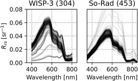
FIGURE 2. Reference R_rs spectra derived from measurements on and around Lake Balaton. There is a difference in normalization between the two data sets, which is discussed in Section 4.3.

The general appearance of the reflectance spectra (Figure 2) is that of a broad peak around 560 nm. On the short wavelength side of this peak, absorption by phytoplankton and CDOM suppresses R_rs to approximately 25% of the peak amplitude. Towards longer wavelengths, the effects of increasing absorption by water are clearly seen around 600 nm and beyond 700 nm, and R_rs reaches near-zero amplitude at the edge of the visible spectrum. The reflectance is ultimately skewed towards blue-green wavelengths, giving the water a turquoise appearance. A minor absorption feature of chl-a and associated accessory pigments is visible around 675 nm. Sun-induced chl-a fluorescence is visible at 680–690 nm in the WISP-3 spectra taken on 4 and 5 July, but not the WISP-3 or So-Rad spectra taken on 3 July.

2.3 Smartphone Data Processing

The RAW smartphone images were processed using a SPECTACLE-based (Burggraaff et al., 2019) pipeline (Figure 3). The images were first corrected for bias or black level, which shifts the pixel values in each image by a constant amount. On the Galaxy S8, the nominal black level was 0 analog-digital units (ADU), while on the iPhone SE it was 528 ADU or 13% of the dynamic range, as determined from the RAW image metadata and validated experimentally (Burggraaff et al., 2019). Next, a flat-field correction was applied, correcting for pixel-to-pixel sensitivity variations. The sensitivity varies by up to 142% across the iPhone SE sensor (Burggraaff et al., 2019), although in the central 100 × 100 pixels, the variations are only 0.2% on the iPhone SE and 1.6% on the Galaxy S8. A central slice of 100 × 100 pixels was taken to decrease the uncertainties introduced by spatial variations across the image (Leeuw and Boss, 2018). The central pixels were then demosaicked into separate images for the RGBG₂ channels, where G₂ is the duplicate green channel present in most consumer cameras (Burggraaff et al., 2019). The RGBG₂ images were flattened into lists of 10,000 samples per channel and normalized by the effective spectral bandwidths of the channels, determined from the SRFs (Burggraaff et al., 2019). The mean radiance was calculated per channel, after which the G and G₂ channels, which have identical SRFs, were averaged together. Finally, R_rs was calculated from L_u, L_sky, and L_d using Eq. 2 (Mobley, 1999). Like for the WISP-3 (Section 2.2) and in HydroColor, a constant ρ = 0.028 was used. R_ref is the gray card reference reflectance, nominally 0.18.

$R_{rs}=\frac{L_u-\rho L_{\mathit{sky}}}{\frac{\pi }{R_{\mathit{ref}}}{L}_d}(2)$

FIGURE 3

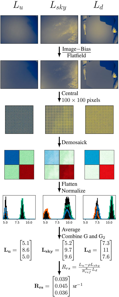
FIGURE 3. Smartphone data processing pipeline, from RAW images to multispectral R_rs. The example input images are those from Figure 1. Some processing steps have been combined for brevity. The histograms show the distribution of normalized pixel values in the central 100 × 100 pixels for the RGBG₂ channels separately (colored lines, G and G₂ combined) and together (black bars). The order of elements in L and R_rs is RGB.

For R_ref, a Brandess Delta 1 18% gray card was used by manually holding it horizontal in front of the camera. The nominal reflectance of R_ref = 18% was verified to within 0.5 percent point in the smartphone RGB bands by comparing spectroradiometer measurements of L_d on a similar gray card to cosine collector measurements of E_d. Angular variations in R_ref were found to be ⪅1 percent point for nadir angles of 35°–45° in a laboratory experiment with the iPhone SE. This value is similar to previous characterizations of different consumer-grade gray cards (Soffer et al., 1995). To account for these factors as well as fouling, an uncertainty of ${\sigma }_{R_{\mathit{ref}}}=0.01$, or 1 percent point, was used in our data processing. This does not account for systematic errors (Section 4.3).

Unlike EyeOnWater, which selects multiple sub-images from different parts of each image, our pipeline only used a central slice of 100 × 100 pixels. The use of sub-images was not necessary since all images were manually curated and sub-imaging has been shown to have little impact on the data quality (Malthus et al., 2020). The 100 × 100 size was chosen to minimize spatial variations, but a comparison of box sizes from 50 to 200 pixels showed that the exact size made little difference. For example, the mean radiance typically varied by $<0.4\%$, less than the typical uncertainty on the radiance estimated from each image (Section 3.1). Furthermore, the signal-to-noise ratio (SNR) varied by $<3\%$ for L_u and L_d but up to 19% in L_sky due to the patchy cloud coverage.

The iPhone SE JPEG data were processed using a simplified version of the RAW pipeline, lacking the bias and flat-field corrections and G-G₂ averaging. Smartphone cameras perform these three tasks internally for JPEG data (Burggraaff et al., 2019). The processing was repeated with an additional linearization step, like in WACODI and EyeOnWater, to determine whether linearization improves the data quality. Following WACODI, the default sRGB inverse gamma curve was used, although this curve has already been shown to be poorly representative of real smartphones (Burggraaff et al., 2019).

The uncertainties in the image data, determined from the sample covariance matrix of the 10,000 pixels per channel per image, were propagated analytically as described in Supplementary Datasheet S1. The pixel values were approximately normally distributed (Figure 3). Significant correlations between the RGBG₂ channels were found. For example, the iPhone SE L_sky image from 3 July 2019 at 07:47 UTC had a correlation of r_RG = 0.68 between R and G, while in the 08:01 image this was only r_RG = 0.09. The observed correlations were likely due to spatial structures in the images (Menon et al., 2007), such as patchy clouds for L_sky and waves for L_u. In larger data sets, the presence of strong correlations could be used as a means to filter out images that are not sufficiently homogeneous. The propagated uncertainties in R_rs were typically 5–10% of the mean R_rs and similarly correlated between channels. For example, the 07:47 data had correlations in R_rs of r_RG = 0.67, r_RB = 0.57, and r_GB = 0.72.

2.4 Color

In addition to absolute R_rs in the RGB bands, several relative color measurements were investigated, namely RGB band ratios, hue angle, and FU index.

The band ratios were calculated as specific combinations of R_rs bands. For simplicity in notation, the ratios are expressed as, for example, G/R instead of R_rs(G)/R_rs(R). Following the literature, the numerators and denominators were chosen as G/R, B/G, and R/B. The G/R ratio is sensitive to water clarity and optical depth (Gao et al., 2022). B/G is sensitive to the chl-a concentration (Goddijn-Murphy et al., 2009), at least in water types where phytoplankton covaries with other absorbing substances. Finally, the R/B ratio is particularly sensitive to broad features such as CDOM absorption, as well as the concentration of scatterers (turbidity, suspended matter concentrations), as described in Hoguane et al. (2012) and Goddijn-Murphy et al. (2009).

To calculate the hue angle, the data were first transformed to the CIE XYZ color space. CIE XYZ is a standard color space representing the colors that a person with average color vision can experience (Sharma, 2003). The reference data were spectrally convolved with the XYZ color matching functions (Nimeroff, 1957). The spectral convolution was applied directly to R_rs, since R_rs represents the true color of the water (Burggraaff, 2020). For the smartphone data, transformation matrices calculated from the smartphone camera SRFs (Supplementary Datasheet S1) were used (Juckett, 2010; Wernand et al., 2013). These matrices are given in Eqs 3, 4. The uncertainties on the matrix elements were not included since this would require a full re-analysis of the raw SRF data (Wyszecki, 1959), which is outside the scope of this work. The resulting colors were relative to an E-type (flat spectrum, x = y = 1/3) illuminant.

${\mathbf{M}}_{RGB\to XYZ}^{iPhoneSE}=\left[\begin{array}{ccc}\hfill 0.5709\hfill & \hfill 0.2452\hfill & \hfill 0.1839\hfill \\ \hfill 0.3760\hfill & \hfill 0.4346\hfill & \hfill 0.1894\hfill \\ \hfill 0.0439\hfill & \hfill 0.0913\hfill & \hfill 0.8648\hfill \end{array}\right](3)$

${\mathbf{M}}_{RGB\to XYZ}^{GalaxyS8}=\left[\begin{array}{ccc}\hfill 0.5611\hfill & \hfill 0.1451\hfill & \hfill 0.2938\hfill \\ \hfill 0.3944\hfill & \hfill 0.2391\hfill & \hfill 0.3666\hfill \\ \hfill 0.0231\hfill & \hfill 0.0416\hfill & \hfill 0.9353\hfill \end{array}\right](4)$

From XYZ, the chromaticity (x, y) and hue angle α were calculated as shown in Eqs 5, 6. Chromaticity is a normalization of the XYZ color space that removes information on brightness (Sharma, 2003). The FU index was determined from α using a look-up table (Novoa et al., 2013; Pitarch et al., 2019). The uncertainties in R_rs were propagated analytically into XYZ and (x, y), as described in Supplementary Datasheet S1. However, further propagation into α was not feasible, since the linear approximation of Eq. 6 breaks down near the white point (x, y) = (1/3, 1/3), especially with highly correlated x and y (Onusic and Mandic, 1989).

$x=\frac{X}{X+Y+Z}y=\frac{Y}{X+Y+Z}(5)$

$\alpha =\mathrm{arctan2}\left(y-1/3,x-1/3\right)\mathrm{mod}2\pi (6)$

2.5 Replicate Analysis

The Galaxy S8 data were taken in sets of 10 sequential replicates per image. The variability between these replicates was analyzed to assess the uncertainty in smartphone data.

The processing chain described in Section 2.3 was applied to each image from each set, resulting in 10 measurements per channel of L_u, L_sky, and L_d. R_rs was calculated from each combination of images, resulting in 1,000 values. From these, the band ratios, α, and FU were calculated.

The relative uncertainty in L_u, L_sky, L_d, R_rs, and the band ratios was estimated through the coefficient of variation $\frac{\sigma }{\mu }$, σ being the standard deviation and μ the mean value. Because α and FU have arbitrary zero-points, relative uncertainties are not applicable to them, and σ was instead used to estimate the absolute uncertainty.

2.6 Match-Up Analysis

Simultaneous data taken with the various sensors were matched up and compared. There were 27 pairs of iPhone SE and Galaxy S8 images, taken on average 50 s apart. On the ferry, which had an average speed of 8 km/h, a 50 s delay corresponded to a distance along the transect of approximately 120 m. The smartphone images were also matched to reference spectra taken within a 10-min time frame, resulting in 1–41 reference spectra per match-up. The reference R_rs spectra were convolved to the smartphone RGB bands by first convolving the reference radiances (Burggraaff, 2020). For match-ups with multiple reference spectra per smartphone image, the median value of each variable in the reference spectra was used, with the standard deviation as an estimate for the uncertainty. For match-ups with a single reference spectrum per smartphone image, the uncertainty was instead estimated as the median uncertainty on the multiple-spectrum match-ups, for each variable. Match-up reference spectra with large uncertainties, for example relative uncertainties of $>10\%$ in R_rs, were not discarded because these represent common measurement scenarios.

The match-up data were compared using the metrics shown in Eqs 7–10. Here P, Q are any two data sets with elements p_i, q_i; cov (P, Q) is their covariance; σ_P, σ_Q are the standard deviations in P and Q, respectively; Med_i is the median evaluated over the indices i; and sgn is the sign function. The RGB channels were treated as separate samples, as were the three band ratios.

$r=\frac{\mathrm{cov}\left(P,Q\right)}{{\sigma }_P{\sigma }_Q}(7)$

$\mathcal{M}={\mathrm{Med}}_i\left(|q_i-p_i|\right)(8)$

$\zeta =\exp \left[{\mathrm{Med}}_i\left(\left|\ln \frac{q_i}{p_i}\right|\right)-1\right](9)$

$\mathcal{B}=\mathrm{sgn}\left[{\mathrm{Med}}_i\left(\ln \frac{q_i}{p_i}\right)\right]\times \left[\exp \left(\left|{\mathrm{Med}}_i\left(\ln \frac{q_i}{p_i}\right)\right|\right)-1\right](10)$

The Pearson correlation r and median absolute deviation $\mathcal{M}$ are well-known (Morley et al., 2018; Seegers et al., 2018). The median symmetric accuracy ζ and signed symmetric percentage bias $\mathcal{B}$, both expressed as a percentage, are recent introductions, which we chose to use for their robustness, symmetry, and ability to span multiple orders of magnitude in the data (Morley et al., 2018). r expresses the degree of linear correlation between variables, from −1 to 1, but is sensitive to outliers and the data range. $\mathcal{M}$ and ζ measure the typical random error or dispersion between variables in absolute and relative terms, respectively. Both are robust to outliers. $\mathcal{B}$ is similar to ζ but measures the bias towards over- or underestimation. The covariance, standard deviations, and median calculated in r and $\mathcal{M}$ were weighted by $w_i=\frac{1}{{\sigma }_{p_i}^2+{\sigma }_{q_i}^2}$. ζ and $\mathcal{B}$ are unweighted.

The FU indices were also compared by the number of matches (Busch J. A. et al., 2016; Seegers et al., 2018), considering both full (ΔFU = 0) and near-matches (ΔFU ≤ 1). The typical uncertainty on human observations is 1 FU (Burggraaff et al., 2021).

5–95% confidence intervals (CIs) on the metrics were estimated by bootstrapping over pairs of (p_i, q_i), and w_i if applicable. Bootstrapping involves randomly resampling the data with replacement, mimicking the original sampling process (Wasserman, 2004). This was necessary to account for the relatively small size of our data set, which increases the effects of outliers, even on robust metrics like $\mathcal{M}$ or ζ. The bootstraps were evaluated with 9,999 resamples, sufficient to obtain consistent results matching the analytical formula for CIs on unweighted r to 4 decimals (Wasserman, 2004).

Some data were also compared through a linear regression (y = ax + b with parameters a, b), to convert data to the same units or account for normalization differences. The regression was done through the scipy.odr function for orthogonal distance regression, which minimizes differences and accounts for weights on both axes. The same process was used to fit a power law (y = ax^b) in the JPEG data comparison (Section 3.4).

3 Results

3.1 Replicate Analysis

The Galaxy S8 replicate analysis showed that among the radiances, L_u had the largest relative variability with a quartile range (QR, the 25–75% percentile range of variability among the sets of replicate observations) of 1.8–5.8%, followed by L_sky with 1.1–3.4%, and L_d with 0.4–1.2% (Figure 4). L_u and L_sky were affected primarily by cloud and wave movement, shaking of the camera, and movement of the ferry on 3 July. Therefore, the variability in L_u and L_sky was largely methodological in nature, as discussed further in Section 4.1. Since L_d was measured on a bright, stable gray card, it was not affected by the above factors, and its variability best represented the radiometric stability of the smartphone camera.

FIGURE 4

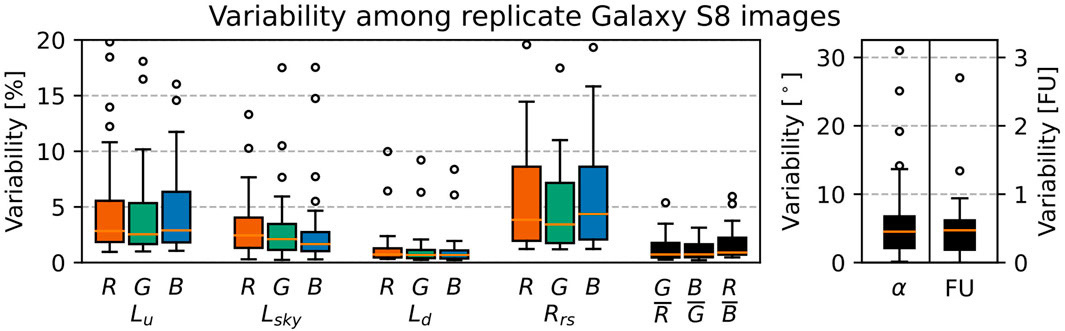
FIGURE 4. Variability in radiance, R_rs, and color between replicate Galaxy S8 images. The boxes show the distribution, among 27 individually processed sets of 10 replicates, of the variability between replicate images. The orange lines indicate the medians, the boxes span the quartile range (QR), the whiskers extend to 1.5 times the QR, and circles indicate outliers. Up to two outliers per column fell outside the y-axis range.

The RGB R_rs varied by 1.9–8.1%, while the R_rs band ratios only varied by 0.5–1.9%. The difference can be explained by correlations between channels. For example, wave movements between successive images affected all three RGB channels of L_u equally, changing the individual R_rs values, but having little effect on their ratios. The same held true for other environmental variations and camera stability issues.

Finally, there was a variability in hue angle α of 2.1°–6.8° and in FU index of 0.19–0.62 FU. The variability distributions of α and FU index did not have the same shape because the hue angle difference between successive FU indices varies greatly.

The variability between replicates represents the typical uncertainty associated with random effects on our data. However, there are some caveats. First, systematic effects such as an error in R_ref would affect successive measurements equally, and not cause random variations. Second, the uncertainty in individual images may be larger due to spatial structures, which the uncertainty propagation described in Section 2.3 does account for. Both of these issues explain differences between the replicate and propagated uncertainties in our data. For example, the propagated uncertainty in individual images was 6.6–9.0% for RGB R_rs and 4.5–7.0% for the band ratios. While the exact uncertainties will differ between campaigns, sites, and even smartphones, the trends seen here can be generalized.

As a point of comparison, the uncertainty QRs for the spectrally convolved WISP-3 data in the Galaxy S8 match-up (Section 3.3), were 4.2–38% in L_u, 4.8–14% in L_sky, 2.5–30% in E_d, 2.6%–7.2% in RGB R_rs, 0.7%–2.9% in R_rs band ratios, 0.4°–2.8° in α, and 0–0.46 in FU. While the Galaxy S8 and WISP-3 variability cannot be compared 1:1 due to differences in data acquisition and processing and in the uncertainty estimation, the order of magnitude of the uncertainties in the Galaxy S8 and WISP-3 reference data was the same.

3.2 Smartphone Comparison

There was a strong correlation, r = 0.94 (CI 0.90, 0.96), between the iPhone SE and Galaxy S8 radiances (Figure 5). Due to differences in exposure settings, both cameras measured radiance in different, arbitrary units (a.u.). After re-scaling the Galaxy S8 data through a linear regression (Section 2.6), the median absolute deviation was $\mathcal{M}=0.39$ (CI 0.29, 0.52) in iPhone SE units and the median symmetric accuracy was ζ = 6.9% (CI 5.1%, 8.7%). The value of ζ was comparable to the variability between replicate images (Section 3.1).

FIGURE 5

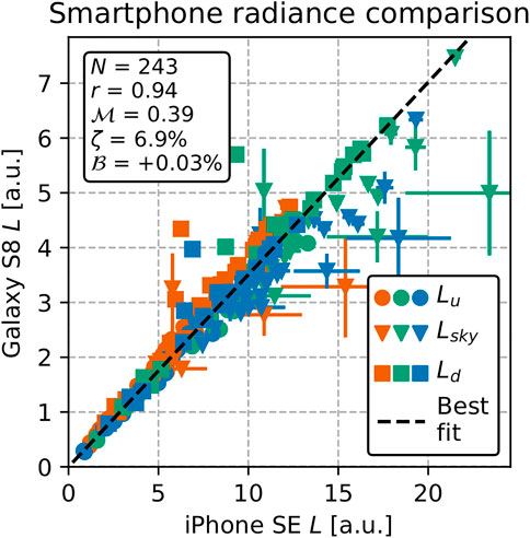
FIGURE 5. Comparison between iPhone SE and Galaxy S8 radiance measurements. The axes are in different units due to differences in exposure settings. The RGB channels are shown in their respective colors, with different symbols for L_u, L_sky, and L_d. The statistics in the text box are relative to the regression line.

The R_rs match-ups between the two smartphones, in both RGB (Figure 6) and band ratios (Figure 7), showed excellent agreement. The data were strongly correlated, with r = 0.98 (CI 0.95, 0.99) for RGB and r = 0.99 (CI 0.99, 1.00) for band ratio R_rs. The typical difference in RGB R_rs was $\mathcal{M}=0.0010$ (CI 0.0005, 0.0013) sr⁻¹ or ζ = 5.5% (CI 3.8%, 8.2%). For band ratios, the typical difference was $\mathcal{M}=0.032$ (CI 0.026, 0.035), unitless, and ζ = 2.9% (CI 2.3%, 3.7%). Both values of ζ are consistent with Section 3.1, as is the observation that band ratios are more reproducible than RGB R_rs. Finally, the signed symmetric percentage bias in RGB R_rs, $\mathcal{B}=-2.7\%$ (CI −7.0%, −1.8%), was smaller than the typical uncertainty. There was no significant offset in the band ratios, with $\mathcal{B}=-1.1\%$ (CI −1.8%, +0.7%).

FIGURE 6

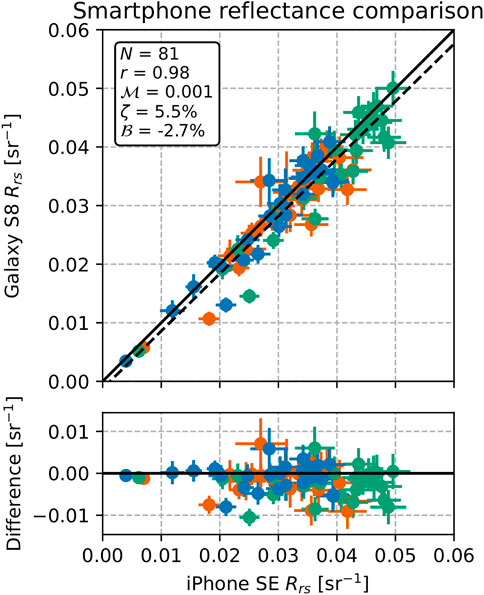
FIGURE 6. Comparison between iPhone SE and Galaxy S8 R_rs measurements in the RGB bands. The solid line corresponds to a 1:1 relation, the dashed line is the best-fitting linear regression line. The statistics in the text box are based on a 1:1 comparison, as are the differences in the lower panel.

FIGURE 7

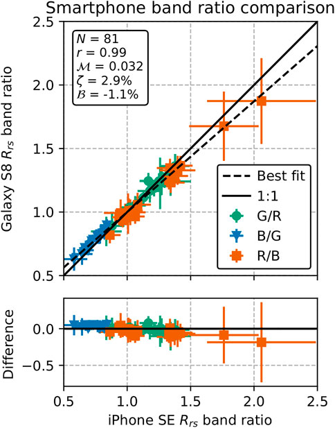
FIGURE 7. Comparison between iPhone SE and Galaxy S8 R_rs band ratios. The solid line corresponds to a 1:1 relation, the dashed line is the best-fitting linear regression line. The statistics in the text box are based on a 1:1 comparison, as are the differences in the lower panel.

The agreement in α and FU was poorer but still similar to the expected uncertainties (Figure 8). The typical difference was $\mathcal{M}={8.3}^{°}$ (CI 5.0°, 11°) in α and $\mathcal{M}=1$ (CI 0, 2) in FU index. 33% (CI 15%, 48%) of the match-up pairs had the same FU index, 59% (CI 37%, 74%) had a difference ΔFU ≤ 1. The wide CIs are due to the relatively small number (N = 27) of match-ups. The data did not span the full range of α, but were mostly concentrated into two clusters, around 50° (FU 14–16, greenish brown) and 90° (FU 8–9, bluish green). Interestingly, while the 90° cluster was centered roughly on the 1:1 line, the 50° cluster fell entirely underneath it. However, due to the small N and the uncertainties on the data, it is difficult to say whether this was significant.

FIGURE 8

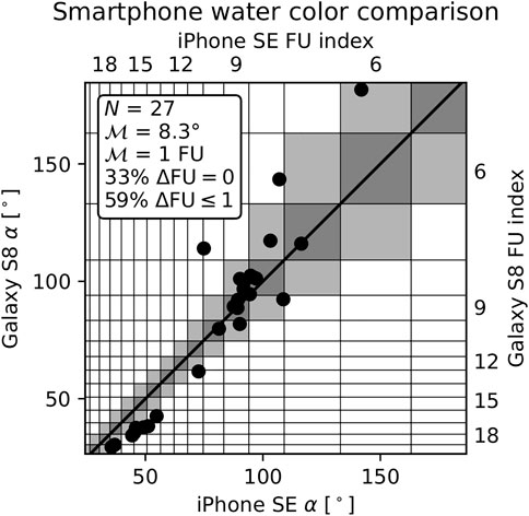
FIGURE 8. Comparison between iPhone SE and Galaxy S8 measurements of hue angle and FU index. The solid line corresponds to a 1:1 relation. The dark gray squares indicate a full FU match, the light gray ones a near-match. Accurate uncertainties on individual points could not be determined (Section 2.4). The statistics in the text box are based on a 1:1 comparison.

3.3 Smartphone vs. Reference Comparison

A total of 72 pairs of smartphone vs. reference match-up spectra were analyzed, four of which are shown in Figure 9. There were 27 match-ups between the WISP-3 and each smartphone and 9 between the So-Rad and each smartphone. Except for the normalization difference that was also present between the So-Rad and WISP-3 (Figure 2, discussed in Section 4.3), there was good agreement between the instruments (Figure 9).

FIGURE 9

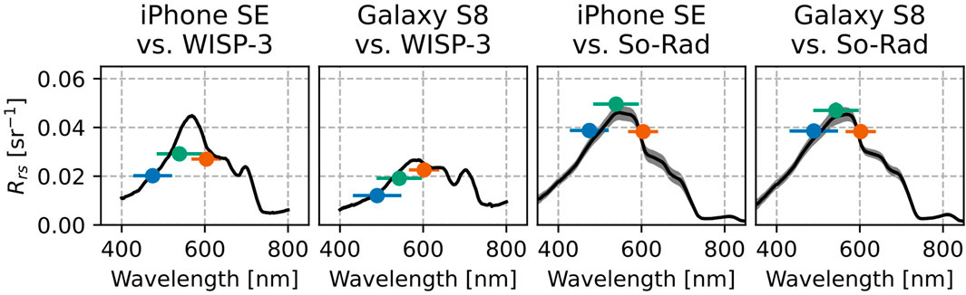
FIGURE 9. Examples of smartphone vs. reference R_rs match-ups at different stations. The solid lines show the reference spectrum, with uncertainties in gray. The RGB dots show the smartphone data, with error bars indicating the effective bandwidth (horizontal) and R_rs uncertainty (vertical). In some panels, the vertical error bars are smaller than the data point size.

The full statistics of the match-up analysis are given in Table 1. The correlation between smartphone and reference radiance was r ≥ 0.71 in all pairs of instruments (Figure 10). The median symmetric accuracy ζ ranged between 12% and 19%, larger than the typical uncertainties and the value from the smartphone vs. smartphone comparison. This larger difference in observed radiance is not surprising, since the smartphone vs. reference match-ups typically differed more in time and location than the smartphone vs. smartphone match-ups. No significant differences in the match-up statistics between the individual RGB bands were found.

TABLE 1

TABLE 1. Summary of the smartphone vs. reference match-up analysis. The values between parentheses indicate the 5–95% CI determined from bootstrapping. N is the number of matching observations; the other metrics are described in Section 2.6. $\mathcal{M}(L)$ is in units of W m⁻² nm⁻¹ sr⁻¹. For the WISP-3, R_rs was compared 1:1 and with a linear regression (regr.).

FIGURE 10

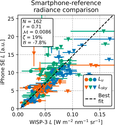
FIGURE 10. Comparison between iPhone SE and spectrally convolved WISP-3 radiance measurements. The RGB channels are shown in their respective colors, with different symbols for L_u and L_sky. The statistics in the text box are relative to the regression line. We note that this regression line cannot be used as a general absolute radiometric calibration for the iPhone SE due to the arbitrary choice of exposure settings.

The RGB R_rs data were strongly correlated between smartphone and reference sensors (r ≥ 0.94 for the WISP-3) and showed a relatively small dispersion, although with a normalization difference in the WISP-3 comparisons (Figure 11), similar to that between the WISP-3 and So-Rad data (Figure 2). To negate the normalization issue, the smartphone data were re-scaled based on a linear regression (Section 2.6) for the smartphone vs. WISP-3 RGB R_rs comparison. The So-Rad and smartphone data were compared 1:1. The typical differences in R_rs, then, were on the order of 10^–3 sr⁻¹ for the So-Rad and 10^–4 sr⁻¹ for the WISP-3, differing mostly due to their different ranges. The difference in range of R_rs also decreased the correlation coefficient r for the So-Rad comparisons. In the four smartphone vs. reference R_rs comparisons, ζ was between 9% and 13%, twice the value seen in the smartphone vs. smartphone comparison but similar to the differences between smartphone and reference radiances.

FIGURE 11

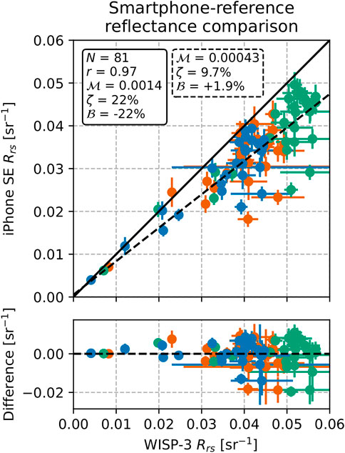
FIGURE 11. Comparison between iPhone SE and spectrally convolved WISP-3 R_rs measurements in the RGB bands. The solid line corresponds to a 1:1 relation, the dashed line is the best-fitting linear regression line. The statistics in the solid-outline text box are based on a 1:1 comparison, those in the dashed-outline text box are based on the regression line. The differences in the lower panel are based on the regression line.

The agreement between smartphone and reference R_rs band ratios was better than the agreement in RGB R_rs (Figure 12). In all four band ratio comparisons, the correlation was near-perfect (r ≥ 0.97), and the typical differences (1.1% ≤ ζ ≤ 3.8%) were consistent with the uncertainties in the data. The WISP-3 normalization difference did not affect this comparison since it divided out.

FIGURE 12

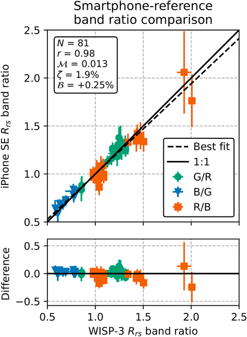
FIGURE 12. Comparison between iPhone SE and spectrally convolved WISP-3 R_rs band ratios. The solid line corresponds to a 1:1 relation, the dashed line is the best-fitting linear regression line. The statistics in the text box are based on a 1:1 comparison, as are the differences in the lower panel.

The agreement in α and FU was not as good as that in L and R_rs, like in the smartphone intercomparison (Section 3.2). For each smartphone, there were only N = 27 WISP-3 match-ups and even fewer So-Rad ones, making the CIs wide and the interpretation difficult. The difference between the WISP-3 and iPhone SE was slightly larger than in the smartphone comparison, at $\mathcal{M}(\alpha )={9.4}^{°}$ (CI 6.3°, 12°) and $\mathcal{M}(\text{FU})=1$ (CI 1, 2). The Galaxy S8 and WISP-3 differed more, at $\mathcal{M}(\alpha )={16}^{°}$ (CI 11°, 21°) and $\mathcal{M}(\text{FU})=2$ (CI 1, 4). The cause for this difference is unclear but may simply be an artifact of the small number of match-ups; the Galaxy S8 also differed more in RGB R_rs but not in the band ratios. Both smartphones performed similarly in the FU match-ups, with 19–26% of the match-ups agreeing fully and 48–59% to within 1 FU, although these figures had particularly wide CIs.

3.4 JPEG Data

28 sets of JPEG images from the iPhone SE, taken simultaneously with the RAW images, were analyzed and compared to the RAW and reference data.

The relationship between JPEG and RAW radiances was highly nonlinear (Figure 13). Each RGB channel had a different best-fitting power law, with exponents ranging from 0.477 ± 0.005 for B to 0.949 ± 0.013 for R. Due to differences between the RAW and JPEG data processing, the power law exponents are not equivalent to sRGB gamma exponents (Burggraaff et al., 2019). Figure 13 also shows the significant dispersion of the data around the power law curves. Comparing the RAW and re-scaled JPEG data yielded ζ ranging from 8.9% (CI 7.5%, 11%) for B to 38% (CI 29%, 43%) for R.

FIGURE 13

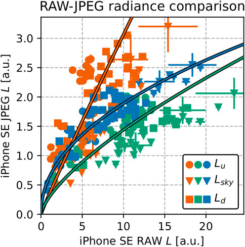
FIGURE 13. Comparison between RAW- and JPEG-based iPhone SE radiance measurements. The axes are in different units due to differences in exposure settings and normalization. The RGB channels are shown in their respective colors, with different symbols for L_u, L_sky, and L_d. The colored lines show the best-fitting power law for each channel.

The JPEG vs. RAW R_rs match-ups agreed better, particularly in the band ratios. The RGB R_rs were strongly correlated, with r = 0.92 (CI 0.84, 0.97), but the JPEG data showed a large, consistent overestimation of $\mathcal{B}=+52\%$ (CI +39%, +59%). Comparing R_rs through a linear regression removed this offset, although a significant dispersion of ζ = 15% (CI 12%, 21%) remained. Conversely, the R_rs band ratios were more similar with r = 0.97 (CI 0.95, 0.98), $\mathcal{M}=0.033$ (CI 0.023, 0.042), and ζ = 4.9% (CI 3.6%, 6.8%).

Finally, the agreement in α and FU was similar to the smartphone vs. smartphone and smartphone vs. reference comparisons. $\mathcal{M}$ was 11° (CI 3.6°, 14°) in α and 1 (CI 0, 2) in FU. 39% (CI 18%, 54%) of match-up pairs had the same FU index, while 61% (CI 39%, 75%) agreed to within 1 FU.

The agreement between JPEG and reference data was notably worse than between RAW and reference data. While the JPEG vs. reference radiance match-ups appeared to follow a single linear relationship, rather than the multiple power laws seen in the JPEG vs. RAW comparison, they were only weakly correlated, with r = 0.39 (CI 0.22, 0.52) in the JPEG vs. WISP-3 comparison. The dispersion around the regression line was ζ = 31% (CI 26%, 41%), 1.6× larger than for the RAW data.

The JPEG data consistently overestimated R_rs compared to the references, and were widely dispersed. In the JPEG vs. WISP-3 comparison, $\mathcal{B}=+17\%$ (CI +10%, +19%), although this was reduced to $\mathcal{B}=+1.1\%$ (CI −7.3%, +5.8%) when comparing to a regression line instead of the 1:1 line, as in Section 3.3. However, the dispersion remained significant at $\mathcal{M}=0.0039$ (CI 0.0018, 0.0047) sr⁻¹ or ζ = 21% (CI 12%, 24%), with $\mathcal{M}9\times$ as much as for the RAW data, and ζ 2.1×.

The JPEG band ratios deviated from the WISP-3 by $>2.5\times$ as much as the RAW data, with $\mathcal{M}=0.032$ (CI 0.023, 0.041) and ζ = 5.5% (CI 3.7%, 6.4%). The So-Rad comparison showed a similarly stark difference. However, while this represents a serious reduction in performance, a typical difference of 5.5% is still relatively small.

It was only in α and FU that the JPEG vs. reference and RAW vs. reference agreements were similar. $\mathcal{M}(\alpha )$ in the JPEG vs. WISP-3 comparison was even marginally better at 7.1° (CI 5.0°, 11°); in the JPEG vs. So-Rad comparison it was 13° (CI 3.8°, 16°), almost identical to Table 1. $\mathcal{M}(\text{FU})$ and the fraction of FU matches were also similar, at $\mathcal{M}(\text{FU})=1$ (CI 1, 2), with 26% (CI 7.4%, 41%) full and 59% (CI 37%, 74%) partial FU matches between the JPEG and WISP-3 data. The agreement between JPEG and reference α and FU is discussed further in Section 4.3.

The effectiveness of an sRGB linearization applied to the JPEG data, like in WACODI, was also investigated (Section 2.3). In α and FU, the main outputs from WACODI, the linearization had very little effect. In the JPEG vs. WISP-3 comparison, $\mathcal{M}(\alpha )$ changed from 7.1° (CI 5.0°, 11°) originally to 7.0° (CI 5.4°, 9.4°) with linearization. In radiance and R_rs, the linearization made all comparison metrics significantly worse.

4 Discussion

4.1 Uncertainty

The uncertainty of the smartphone data as derived from replicate measurements (Section 3.1) is comparable to that of professional spectroradiometers. This was shown by the comparison with WISP-3 replicate measurements, which had a variability similar to, and in some cases larger than, the Galaxy S8. In general, the uncertainty from instrumental effects, excluding environmental factors and photon noise, in professional spectroradiometer data is around 1% (Vabson et al., 2019). In field data, the typical uncertainty is 1–7% (Białek et al., 2020). The Galaxy S8 replicate variability, which was 0.4–1.2% (L_d), 1.1–3.4% (L_sky), and 1.8–5.8% (L_u), falls within this range.

The same is true for the smartphone R_rs uncertainty, both in RGB (1.9–8.1%) and in band ratios (0.5–1.9%). R_rs is typically measured with an uncertainty of 5% at blue and green wavelengths (IOCCG, 2019) and this is the target for satellites like PACE (Werdell et al., 2019). The 5% target also applies to narrower bands than the smartphone SRFs and to waters considerably darker than Lake Balaton, which increases the influence of sensor noise. The reduced uncertainty in band ratios is well-known and can be attributed to correlated uncertainties dividing out (Lee et al., 2014). Propagated into the mineral suspended sediment (MSS) algorithm described in Hoguane et al. (2012), for R/B ranging from 1.0 to 1.4, a 2% uncertainty in R/B results in a relative MSS uncertainty of only 1%. In the chl-a algorithm from Goddijn-Murphy et al. (2009), a 2% uncertainty in B/G induces a relative chl-a uncertainty of 9%. This level of uncertainty is well within the desired limits for many end users (IOCCG, 2019).

Finally, the uncertainty of the Galaxy S8 α (2.1°–6.8°) and FU index (0.19–0.62 FU) estimates is similar to the uncertainty of satellite and human measurements as well as the existing EyeOnWater app. Through propagation from R_rs, Pitarch et al. (2019) found uncertainties on SeaWiFS-derived α of 6°–18°, although it is difficult to compare these values due to the vastly different water types examined. Furthermore, propagated and replicate-based uncertainty estimates may vary significantly due to differences in sensitivity to various factors (Section 3.1). A more representative comparison point is the standard deviation of 3.15° among replicate EyeOnWater observations by Malthus et al. (2020), which falls squarely within the range found in this work. The similarity in uncertainty is interesting because EyeOnWater is based on JPEG data, not RAW. However, since we did not take replicate JPEG images, a direct comparison in uncertainty between JPEG and RAW could not be made. The accuracy of JPEG and RAW data, including α and FU index, is compared in Section 4.3. The uncertainty of 0.19–0.62 FU is 5.3–1.6× better than human measurements, which have a typical uncertainty of 1 FU with perfect color vision (Burggraaff et al., 2021).

Since the use of RAW data eliminates virtually all smartphone-specific sources of uncertainty (Burggraaff et al., 2019), the primary remaining sources are those that apply to all (spectro)-radiometers as well as environmental factors. For a thorough overview of the former, we refer the reader to Białek et al. (2020) and Mittaz et al. (2019); for the latter, to IOCCG (2019). Read-out noise, thermal dark current, and digitization noise are negligible for well-lit smartphone images (Burggraaff et al., 2019). Since L_d was measured on a stable target, its variability of 0.4–1.2% between replicates can be ascribed mostly to sensor noise (Section 3.1). Sensor noise scales with the square root of the number of photons, so the induced uncertainty will be larger in darker conditions such as overcast days, highly absorbing waters, and low solar elevation angles. In practice, smartphone observations under dark conditions will require longer exposure times or multiple images to attain similar levels of uncertainty. The impact of sun glint, which is estimated from L_sky, on the uncertainty in R_rs is also larger for darker waters. The sensitivity of smartphone cameras to temperature variations and polarization is unknown, although the latter is expected to be negligible unless special fore-optics are used (Burggraaff et al., 2020). Because our data were gathered in a single 3-days campaign, long-term sensor drift is unlikely to have had any effect; in general, sensor drift does not affect relative measurements like R_rs and α. Environmental factors, such as the patchy clouds that were present during our campaign (Figure 1), likely contributed the bulk of the uncertainty in L_sky and L_u. These environmental factors also affected the reference measurements and are inherent to above-water radiometry.

4.2 Reproducibility

As there are hundreds of different smartphone models, reproducibility between devices is key. This is a major problem with HydroColor, as reported to us directly by users and as reported in the literature. For example, HydroColor measurements of R_rs with different smartphones regularly differ by as much as 50% or 0.005 sr⁻¹ (Leeuw and Boss, 2018; Yang et al., 2018). This is largely due to the use of JPEG data, which are processed differently on every smartphone model, leading to a wide variety of errors and uncertainties that cannot be reliably corrected (Burggraaff et al., 2019). On the other hand, Goddijn-Murphy et al. (2009) reported smaller differences (4 ± 4%) between JPEG data from two high-quality digital cameras, suggesting that some of the problems may be specific to smartphones.

In Section 3.2, we showed that with RAW data and camera calibrations, excellent agreement and thus reproducibility between smartphones can be achieved. Near-simultaneous iPhone SE and Galaxy S8 measurements of radiance and R_rs were nearly perfectly correlated (r ≥ 0.94), and their dispersion could be explained by the uncertainties in the individual measurements. The typical difference in R_rs was 0.0010 (CI 0.0005, 0.0013) sr⁻¹ or 5.5% (CI 3.8%, 8.2%), both major improvements over HydroColor. In fact, the dispersion in radiance between the two smartphones, ζ = 6.9% (CI 5.1%, 8.7%), is only slightly larger than that between professional instruments in a similar experiment (Vabson et al., 2019).

On the contrary, the smartphone JPEG processing algorithm was found to be poorly constrained and highly inconsistent between the RGB channels (Section 3.4). Moreover, the internal JPEG processing in the smartphone is re-tuned every time a camera session is started (Burggraaff et al., 2019). Combined, the differences between channels and between sessions highly limit the reproducibility of JPEG-based measurements of radiance and R_rs. As discussed below, white-balancing further reduces the reproducibility of JPEG-based R_rs band ratios and hue angles. Finally, the JPEG processing algorithms differ between manufacturers, further reducing the reproducibility of JPEG data between devices (Burggraaff et al., 2019). Due to limitations in the SPECTACLE app in 2019, we did not collect Galaxy S8 JPEG data in this study, meaning a direct comparison between the RAW vs. RAW and JPEG vs. JPEG reproducibility could not be performed. Reproducing JPEG data from the RAW data was not possible, due to the aforementioned proprietary smartphone algorithms.

Differences in smartphone SRFs set some minor fundamental limits on the reproducibility between different cameras (Nguyen et al., 2014). However, since most natural waters have broad and smooth spectra, this should only lead to minor differences. In theory, JPEG data do not have this problem because they are always in the sRGB color space (Novoa et al., 2015), but in practice the various proprietary color algorithms cause larger differences in JPEG data than in RAW (Burggraaff et al., 2019). Furthermore, to account for illumination differences, JPEG data are white-balanced, changing the relative intensity of each channel. The re-normalization directly reduces the accuracy of band ratio and hue angle measurements and is difficult to correct post-hoc (Burggraaff et al., 2019; Gao et al., 2022). The white-balance setting may be locked between exposures (Goddijn-Murphy et al., 2009; Leeuw and Boss, 2018), but this does not guarantee consistency between different devices. Finally, due to differences in field-of-view between cameras, the central slice of 100 × 100 pixels does not always subtend the same solid angle. In future work, it may be advisable to use a constant solid angle rather than a constant pixel slice (Leeuw and Boss, 2018).

4.3 Accuracy

In Section 3.3, we compared smartphone and reference data to determine the accuracy of the smartphone data, but this comes with important caveats. While each instrument measured L_u and L_sky, they did not do so in exactly the same way, having differences in field of view, spectral response, spectral resolution, and time and location. While the smartphones measured L_d on a gray card, the references measured E_d with a cosine collector. Due to these differences, the true “ground truth” value of each measurand is not known (Mittaz et al., 2019; Woodhouse, 2021). The reference data can be used to approximate the true values and achieve closure (Werdell et al., 2018), but one must be aware of the uncertainties and systematic errors that may be present. Additionally, one must exercise caution when comparing different metrics, such as the median symmetric accuracy ζ and the mean percentage deviation, which measure the same quantity but are calculated differently and on different data.

The WISP-3 and So-Rad R_rs spectra were similarly shaped, but differently normalized (Section 2.2). Both were similar to spectra from previous work in shape, with the So-Rad more similar in magnitude (Palmer, 2015; Riddick, 2016). Normalization differences and offsets have been seen in previous comparisons between the WISP-3 and other instruments (Hommersom et al., 2012; Vabson et al., 2019), so we felt confident in using a linear regression to re-scale R_rs in the smartphone vs. WISP-3 comparisons. In fact, since each smartphone R_rs measurement was based on three images from the same camera, rather than from three separate sensors like the WISP-3, and the gray card reference was independently verified, we can be more confident in the normalization of the smartphone R_rs than that of the WISP-3, at least for the particular unit and calibration settings used during our campaign. These results suggest that smartphones and other low-cost cameras could be used to provide closure when there is tension between data from professional instruments (Section 4.5).

Considering the above, the level of closure between smartphone and reference data was comparable to intercomparisons between professional radiometers to within a factor of 2–3. The dispersion ζ in radiance was relatively large at 12–19%, 2–3× that reported in a comparison of hyperspectral instruments on a single, stable platform (Vabson et al., 2019), but as discussed previously, our radiance measurements were particularly affected by environmental factors and were taken at slightly different times and positions between instruments. Patchy clouds can increase the dispersion in radiance match-ups by a factor of 10 or more (Hommersom et al., 2012). In R_rs, the typical difference was on the order of 10⁻⁴–10⁻³ sr⁻¹ or 9–13%. Comparing hyperspectral radiometers, Tilstone et al. (2020) found mean differences between sensors on the order of 10^–3 sr⁻¹ or 1–8%, with outliers up to 13%. A comparison between WISP-3 and RAMSES sensors under cloudy conditions, similar to ours, found differences in R_rs of 20–30% (Hommersom et al., 2012).

Most importantly, the smartphone and reference measurements of R_rs band ratios agreed to within 2% in three out of four comparisons. The difference was only larger in the iPhone SE vs. So-Rad comparison, at 3.8%. Since band ratios are what most inversion algorithms for inherent optical properties and constituent concentrations are based on, it is the band ratio accuracy that determines the usefulness of smartphones as spectroradiometers. An accuracy and uncertainty of around 2% is well within most user requirements (Section 4.1).

The accuracy of the JPEG data was considerably worse (Section 3.4). In R_rs, the dispersion in the JPEG vs. WISP-3 comparison was 0.0039 (CI 0.0018, 0.0047) sr⁻¹ or 21% (CI 12%, 24%), which is in line with previous validation efforts for HydroColor (Leeuw and Boss, 2018; Yang et al., 2018) and other JPEG-based methods (Gao et al., 2020, 2022). At $\mathcal{M}=0.032$ (CI 0.023, 0.041) and ζ = 5.5% (CI 3.7%, 6.4%), the same is true for the R_rs band ratios (Yang et al., 2018). The RAW data performed better on each of these metrics, most notably by 9× for the RGB R_rs and 2.5× for the band ratios. These results do not completely invalidate previous JPEG-based methods nor HydroColor specifically (Malthus et al., 2020), but demonstrate the significant increase in accuracy and decrease in uncertainty obtained by using RAW data.

The results for the hue angle α and FU index were less conclusive. While at first glance the dispersion of approximately 10° or 1 FU appears to be in line with previous studies (Novoa et al., 2015; Busch J. A. et al., 2016; Malthus et al., 2020), our measurement protocol did not follow the EyeOnWater protocol exactly, so the results cannot be compared directly to the aforementioned validation efforts. Additionally, our data only contained 27 smartphone vs. WISP-3 match-ups and even fewer for the So-Rad, with little diversity. Lastly, hue angles derived from narrow-band multispectral satellite data have been shown to differ systematically by several degrees, up to 20° in extreme cases, compared to hue angles derived from hyperspectral data (van der Woerd and Wernand, 2018; Pitarch et al., 2019). This effect may also be present in the smartphone data and a correction term in the hue angle algorithm may be necessary (van der Woerd and Wernand, 2015). This work used the original hue angle algorithm, which is based only on the SRFs (Wernand et al., 2013), to enable a comparison between RAW and JPEG data and between the current study and previous works, particularly the WACODI algorithm (Novoa et al., 2015). We recommend that future work be done to investigate the magnitude of the hue angle bias in consumer camera data. Interestingly, there was little difference in accuracy between the RAW- and JPEG-derived hue angles and FU indices. It is unclear whether this is because the method is inherently robust to JPEG-induced errors (Novoa et al., 2015), although Gao et al. (2022) have suggested that it is not. More data, from more diverse waters, will be necessary to compare the accuracy of RAW- and JPEG-based hue angles and FU indices.

A potentially important source of systematic error is the 18% gray card. While the gray card used here did not deviate significantly from R_ref = 18% (Section 2.3), this may not be true in general. Since many smartphone radiometry projects are aimed at citizen scientists, who may purchase a wide variety of gray cards and may not always use them correctly, this presents an important possible source for error. Even a small difference in R_ref can significantly bias R_rs. One possible solution to this problem is to issue or recommend standardized gray cards (Gao et al., 2022). Characterizing the most popular gray cards is another possibility (Soffer et al., 1995), which may itself be done through citizen science. The use of relative quantities like band ratios negates this problem.

4.4 Recommendations

Based on previous work and the results discussed above, several recommendations can be made. Some are specific to smartphones, but most apply in general to above-water radiometry with consumer cameras since the cameras in most smartphones, digital cameras, UAVs, and webcams are extremely similar (Burggraaff et al., 2019).

RAW data provide professional-grade radiometric performance and should be used whenever possible. Most consumer cameras now support this natively and many smartphone apps provide this capacity. Within the MONOCLE³ project, a universal smartphone library for RAW acquisition and processing is in development. In the future, apps like HydroColor may simply import this library and use RAW data without further work from the user. The SPECTACLE Python library (Section 2.3) provides this functionality on PCs.

Few calibration data are necessary for above-water radiometry. Our processing pipeline contains bias and flatfield corrections, demosaicks the data to the RGBG₂ channels, and normalizes by the SRF spectral bandwidths (Figure 3). RAW files from virtually all cameras contain metadata describing the bias correction and demosaicking pattern. The flatfield correction requires additional data, which can be obtained through do-it-yourself methods (Burggraaff et al., 2019), but may also be neglected at little cost in accuracy because its effect is typically small (0.2% for the iPhone SE and 1.6% for the Galaxy S8) in the central 100 × 100 pixels. The flat-field correction is more important in approaches that require a wider field-of-view like the multiple gray card approach (Gao et al., 2022). The bandwidth normalization divides out in the calculation of R_rs and thus is only necessary to obtain accurate radiances. The SRFs are also required to accurately calculate α and convolve hyperspectral data in validation efforts, but may be approximated by standard profiles (Leeuw and Boss, 2018). Low-cost smartphone spectrometers and other novel methods will soon enable on-the-fly SRF calibrations (Burggraaff et al., 2020; Tominaga et al., 2022).

As discussed in Burggraaff et al. (2019), it is important to accurately record exposure settings. In the current study, the exposure settings were not recorded, so it is not possible to combine our data with data from other studies, taken with different settings. The most important exposure settings are ISO speed and exposure time, which strongly affect the observed signal, but are not recorded accurately in the image metadata (EXIF). The settings must therefore be recorded by the user or the app. Since ISO speed does not affect the signal-to-noise ratio (SNR), a constant value maybe used. Longer exposure times increase the SNR but run the risk of saturation. Ideally, an automatic exposure time is determined and recorded for each image; if this is not possible, a single value may be used.

Algorithms to retrieve inherent optical properties from smartphone-based R_rs measurements are best based on band ratios since they are the most precise, reproducible, and accurate. Algorithms based on absolute R_rs in RGB (Leeuw and Boss, 2018; Gao et al., 2022) are more susceptible to uncertainty and systematic errors. Because the RGB SRFs are broad and overlapping, some narrow spectral features like pigment absorption peaks cannot be distinguished, and retrieval algorithms require tuning to specific sites (Hoguane et al., 2012). In edge cases where spectral features fall on wavelengths where SRFs vary significantly between devices, the reproducibility of retrieval algorithms between devices may also vary. For example, the iPhone SE and Galaxy S8 B-band SRFs differ greatly between 550 and 600 nm (Burggraaff et al., 2019). Algorithms that use spectrally distinct peaks, for example to retrieve chl-a concentrations, should be unaffected. Distinguishing between chl-a and CDOM, which both absorb in the B and G bands, may require a three-band algorithm that also estimates the backscattering coefficient b_b from the R-band (Hoge and Lyon, 1996). Alternative color spaces like relative RGB (Hoguane et al., 2012; Iwaki et al., 2021), hue-saturation-intensity (Hatiboruah et al., 2020), and CIE L*a*b* (Watanabe et al., 2016) are also worth exploring. Potential algorithms may be identified through spectral convolution of archival R_rs spectra (Burggraaff, 2020).

4.5 Outlook

The findings presented in this work extend to other methods for smartphone (spectro)radiometry and to most consumer cameras. This study was performed as a precursor to the field validation for the iSPEX 2 smartphone spectropolarimeter (Burggraaff et al., 2020). The uncertainty, accuracy, and reproducibility of iSPEX 2 data will be comparable to what was found in this study, although longer exposure times will be necessary to attain similar photon counts. The low uncertainty and high accuracy of the R_rs band ratios is particularly promising since iSPEX 2 will measure hyperspectrally across the visible range, enabling many such algorithms. Also applicable to iSPEX 2 are some of the limitations found in this work, primarily the dependence on a gray card and the question of sensitivity in low-light conditions.

There is also potential for low-cost cameras, like webcams and UAV cameras, to augment professional spectroradiometers. Removal of the direct sun glint remains challenging, requiring assumptions about the spectrum and wave statistics (Groetsch et al., 2017; Ruddick et al., 2019). Low-cost camera images, taken simultaneously with the spectra, could be used to determine the wave statistics akin to Cox and Munk (1954) but for individual exposures. A similar system, which flags spectra if the associated image has saturated pixels, was already demonstrated in Garaba et al. (2012), and there are further opportunities for image-based anomaly detection. Finally, low-cost cameras can serve as simple validation checks for other sensors, for example to identify normalization problems.

5 Conclusion

In this work, we have assessed the performance of smartphones as multispectral above-water radiometers. We have extended the existing smartphone-based approaches by using RAW data, processed through the SPECTACLE method for calibration of consumer cameras (Burggraaff et al., 2019). Using field data gathered under realistic observing conditions on and around Lake Balaton, we have analyzed the uncertainty, reproducibility, and accuracy of above-water radiometry data taken with smartphone cameras. Furthermore, by comparing RAW and JPEG data, we have determined to what extent our new method improves upon existing work.

The uncertainty of the smartphone data, determined from replicate observations, was on the percent level and was comparable to professional radiometers. The typical uncertainty on R_rs band ratios was 0.5–1.9%, leading to percent-level uncertainties in retrieved inherent optical properties and constituent concentrations. This level of uncertainty falls within the desired limits for many end users.

The reproducibility between smartphones was excellent, representing a significant improvement over existing methods, in some cases nearly tenfold. Any differences in the data between smartphones could be explained by measurement uncertainties.

The accuracy of smartphone data, as determined from match-ups with reference instruments, was comparable to professional instruments. The typical difference between smartphone and reference instruments was 10⁻⁴–10⁻³ sr⁻¹ or 9–13% in RGB R_rs, and 0.004–0.013 or 1.1–3.8% in R_rs band ratios. These differences were an improvement of 9× and 2.5×, respectively, over JPEG data.

Based on the findings of this study, we recommend the use of RAW data for above-water radiometry with smartphones by professional and citizen scientists alike. We further recommend that retrieval algorithms be based on R_rs band ratios rather than absolute RGB R_rs. Potential algorithms may be identified through spectral convolution of archival hyperspectral data. The conclusions and recommendations described above extend to other consumer cameras and to hyperspectral approaches like iSPEX 2. Future work should focus on determining the limitations of consumer cameras, primarily in terms of sensitivity, and exploring opportunities for complementary use of consumer cameras and professional spectroradiometers.

Data Availability Statement

The datasets presented in this study can be found in online repositories. The names of the repository/repositories and accession number(s) can be found below: Zenodo, https://doi.org/10.5281/zenodo.4549621.

Author Contributions

OB, EB, and FS formulated the original concept for this study. OB, MW, EB, and SS collected the in situ data. OB implemented the data processing and analysis. MW, EB, SS, and FS advised on the analysis. OB drafted the manuscript. All authors contributed to the final manuscript and gave final approval for publication.

Funding

This project has received funding from the European Union’s Horizon 2020 research and innovation programme under grant agreement No 776480.

Conflict of Interest

The authors declare that the research was conducted in the absence of any commercial or financial relationships that could be construed as a potential conflict of interest.

Publisher’s Note

All claims expressed in this article are solely those of the authors and do not necessarily represent those of their affiliated organizations, or those of the publisher, the editors and the reviewers. Any product that may be evaluated in this article, or claim that may be made by its manufacturer, is not guaranteed or endorsed by the publisher.

Acknowledgments

The authors would like to thank Tom Jordan, Victor Martínez-Vicente, Aser Mata, Caitlin Riddick, Norbert Schmidt, and Anna Windle for their help in the data acquisition and processing, and Thomas Leeuw, Sanjana Panchagnula, and Hans van der Woerd for valuable discussions relating to this work.

Supplementary Material

The Supplementary Material for this article can be found online at: https://www.frontiersin.org/articles/10.3389/frsen.2022.940096/full#supplementary-material

Footnotes

¹https://github.com/burggraaff/smartphone-water-colour

²https://dx.doi.org/10.5281/zenodo.4549621

³https://monocle-h2020.eu/

References

Al-Ghifari, K., Nurdjaman, S., Dika Praba P Cahya, B., Nur, S., Widiawan, D. A., and Jatiandana, A. P. (2021). Low Cost Method of Turbidity Estimation Using A Smartphone Application in Cirebon Waters, Indonesia. Borneo J. Mar. Sci. Aqua 5, 32–36. doi:10.51200/bjomsa.v5i1.2713

CrossRef Full Text | Google Scholar

Andrachuk, M., Marschke, M., Hings, C., and Armitage, D. (2019). Smartphone Technologies Supporting Community-Based Environmental Monitoring and Implementation: a Systematic Scoping Review. Biol. Conserv. 237, 430–442. doi:10.1016/j.biocon.2019.07.026

CrossRef Full Text | Google Scholar

Ayeni, A. O., and Odume, J. I. (2020). Analysis of Algae Concentration in the Lagos Lagoon Using Eye on Water and Algae Estimator Mobile App. FUTY J. Environ. 14, 105–115.

Google Scholar

Białek, A., Douglas, S., Kuusk, J., Ansko, I., Vabson, V., Vendt, R., et al. (2020). Example of Monte Carlo Method Uncertainty Evaluation for Above-Water Ocean Colour Radiometry. Remote Sens. 12, 780. doi:10.3390/rs12050780

CrossRef Full Text | Google Scholar

Burggraaff, O. (2020). Biases from Incorrect Reflectance Convolution. Opt. Express 28, 13801–13816. doi:10.1364/OE.391470

PubMed Abstract | CrossRef Full Text | Google Scholar

Burggraaff, O., Panchagnula, S., and Snik, F. (2021). Citizen Science with Colour Blindness: A Case Study on the Forel-Ule Scale. PLOS ONE 16, e0249755. doi:10.1371/journal.pone.0249755

PubMed Abstract | CrossRef Full Text | Google Scholar

Burggraaff, O., Perduijn, A. B., van Hek, R. F., Schmidt, N., Keller, C. U., and Snik, F. (2020). A Universal Smartphone Add-On for Portable Spectroscopy and Polarimetry: iSPEX 2. Proc. SPIE (SPIE) 11389, 113892K. doi:10.1117/12.2558562

CrossRef Full Text | Google Scholar

Burggraaff, O., Schmidt, N., Zamorano, J., Pauly, K., Pascual, S., Tapia, C., et al. (2019). Standardized Spectral and Radiometric Calibration of Consumer Cameras. Opt. Express 27, 19075–19101. doi:10.1364/OE.27.019075

PubMed Abstract | CrossRef Full Text | Google Scholar

Busch, J. A., Price, I., Jeansou, E., Zielinski, O., and van der Woerd, H. J. (2016). Citizens and Satellites: Assessment of Phytoplankton Dynamics in a NW Mediterranean Aquaculture Zone. Int. J. Appl. Earth Observation Geoinformation 47, 40–49. doi:10.1016/j.jag.2015.11.017

CrossRef Full Text | Google Scholar

Busch, J., Bardaji, R., Ceccaroni, L., Friedrichs, A., Piera, J., Simon, C., et al. (2016). Citizen Bio-Optical Observations from Coast- and Ocean and Their Compatibility with Ocean Colour Satellite Measurements. Remote Sens. 8, 879. doi:10.3390/rs8110879

CrossRef Full Text | Google Scholar

Cox, C., and Munk, W. (1954). Measurement of the Roughness of the Sea Surface from Photographs of the Sun's Glitter. J. Opt. Soc. Am. 44, 838–850. doi:10.1364/JOSA.44.000838

CrossRef Full Text | Google Scholar

Friedrichs, A., Busch, J., van der Woerd, H., and Zielinski, O. (2017). SmartFluo: A Method and Affordable Adapter to Measure Chlorophyll a Fluorescence with Smartphones. Sensors 17, 678. doi:10.3390/s17040678

PubMed Abstract | CrossRef Full Text | Google Scholar

Gallagher, J. B., and Chuan, C. H. (2018). Chlorophyll a and Turbidity Distributions: Applicability of Using a Smartphone "App" across Two Contrasting Bays. J. Coast. Res. 345, 1236–1243. doi:10.2112/JCOASTRES-D-16-00221.1

CrossRef Full Text | Google Scholar

Gao, M., Li, J., Wang, S., Zhang, F., Yan, K., Yin, Z., et al. (2022). Smartphone-Camera-Based Water Reflectance Measurement and Typical Water Quality Parameter Inversion. Remote Sens. 14, 1371. doi:10.3390/rs14061371

CrossRef Full Text | Google Scholar

Gao, M., Li, J., Zhang, F., Wang, S., Xie, Y., Yin, Z., et al. (2020). Measurement of Water Leaving Reflectance Using a Digital Camera Based on Multiple Reflectance Reference Cards. Sensors 20, 6580. doi:10.3390/s20226580

PubMed Abstract | CrossRef Full Text | Google Scholar

Garaba, S. P., Schulz, J., Wernand, M. R., and Zielinski, O. (2012). Sunglint Detection for Unmanned and Automated Platforms. Sensors 12, 12545–12561. doi:10.3390/s120912545

CrossRef Full Text | Google Scholar

Garcia-Soto, C., Seys, J. J. C., Zielinski, O., Busch, J. A., Luna, S. I., Baez, J. C., et al. (2021). Marine Citizen Science: Current State in Europe and New Technological Developments. Front. Mar. Sci. 8, 621472. doi:10.3389/fmars.2021.621472

CrossRef Full Text | Google Scholar

Goddijn-Murphy, L., Dailloux, D., White, M., and Bowers, D. (2009). Fundamentals of In Situ Digital Camera Methodology for Water Quality Monitoring of Coast and Ocean. Sensors 9, 5825–5843. doi:10.3390/s90705825

PubMed Abstract | CrossRef Full Text | Google Scholar

Groetsch, P. M. M., Gege, P., Simis, S. G. H., Eleveld, M. A., and Peters, S. W. M. (2017). Validation of a Spectral Correction Procedure for Sun and Sky Reflections in Above-Water Reflectance Measurements. Opt. Express 25, A742–A761. doi:10.1364/OE.25.00A742

PubMed Abstract | CrossRef Full Text | Google Scholar

Harris, C. R., Millman, K. J., van der Walt, S. J., Gommers, R., Virtanen, P., Cournapeau, D., et al. (2020). Array Programming with NumPy. Nature 585, 357–362. doi:10.1038/s41586-020-2649-2

PubMed Abstract | CrossRef Full Text | Google Scholar

Hatiboruah, D., Das, T., Chamuah, N., Rabha, D., Talukdar, B., Bora, U., et al. (2020). Estimation of Trace-Mercury Concentration in Water Using a Smartphone. Measurement 154, 107507. doi:10.1016/j.measurement.2020.107507

CrossRef Full Text | Google Scholar

Hoge, F. E., and Lyon, P. E. (1996). Satellite Retrieval of Inherent Optical Properties by Linear Matrix Inversion of Oceanic Radiance Models: An Analysis of Model and Radiance Measurement Errors. J. Geophys. Res. 101, 16631–16648. doi:10.1029/96JC01414

CrossRef Full Text | Google Scholar

Hoguane, A. M., Green, C. L., Bowers, D. G., and Nordez, S. (2012). A Note on Using a Digital Camera to Measure Suspended Sediment Load in Maputo Bay, Mozambique. Remote Sens. Lett. 3, 259–266. doi:10.1080/01431161.2011.566287

CrossRef Full Text | Google Scholar

Hommersom, A., Kratzer, S., Laanen, M., Ansko, I., Ligi, M., Bresciani, M., et al. (2012). Intercomparison in the Field between the New WISP-3 and Other Radiometers (TriOS Ramses, ASD FieldSpec, and TACCS). J. Appl. Remote Sens. 6, 063615. doi:10.1117/1.JRS.6.063615

CrossRef Full Text | Google Scholar

IOCCG (2019). “Uncertainties in Ocean Colour Remote Sensing,” in Vol. 18 of Reports of the International Ocean Colour Coordinating Group (Dartmouth, Canada: IOCCG). doi:10.25607/OBP-696

CrossRef Full Text | Google Scholar

IOCCG (2008). “Why Ocean Colour? the Societal Benefits of Ocean-Colour Technology,” in Vol. 7 of Reports of the International Ocean Colour Coordinating Group (Dartmouth, Canada: IOCCG). doi:10.25607/OBP-97

CrossRef Full Text | Google Scholar

Iwaki, M., Takamura, N., Nakada, S., and Oguma, H. (2021). Monitoring of Lake Environment Using a Fixed Point and Time-Lapse Camera — Case Study of South Basin of Lake Biwa. J. Remote Sens. Soc. Jpn. 41, 563–574. doi:10.11440/rssj.41.563

CrossRef Full Text | Google Scholar

Jordan, T. M., Simis, S. G. H., Grötsch, P. M. M., and Wood, J. (2022). Incorporating a Hyperspectral Direct-Diffuse Pyranometer in an Above-Water Reflectance Algorithm. Remote Sens. 14, 2491. doi:10.3390/rs14102491

CrossRef Full Text | Google Scholar

[Dataset] Juckett, R. (2010). RGB Color Space Conversion. Available at: https://www.ryanjuckett.com/rgb-color-space-conversion/.

Google Scholar

Lee, Z., Shang, S., Hu, C., and Zibordi, G. (2014). Spectral Interdependence of Remote-Sensing Reflectance and its Implications on the Design of Ocean Color Satellite Sensors. Appl. Opt. 53, 3301–3310. doi:10.1364/AO.53.003301

PubMed Abstract | CrossRef Full Text | Google Scholar

Leeuw, T., and Boss, E. (2018). The HydroColor App: Above Water Measurements of Remote Sensing Reflectance and Turbidity Using a Smartphone Camera. Sensors 18, 256. doi:10.3390/s18010256

PubMed Abstract | CrossRef Full Text | Google Scholar

Lim, H. S., Mat Jafri, M. Z., Abdullah, K., and Abu Bakar, M. N. (2010). Water Quality Mapping Using Digital Camera Images. Int. J. Remote Sens. 31, 5275–5295. doi:10.1080/01431160903283843

CrossRef Full Text | Google Scholar

Malthus, T. J., Ohmsen, R., and van der Woerd, H. J. (2020). An Evaluation of Citizen Science Smartphone Apps for Inland Water Quality Assessment. Remote Sens. 12, 1578. doi:10.3390/rs12101578

CrossRef Full Text | Google Scholar

Menon, D., Andriani, S., and Calvagno, G. (2007). Demosaicing with Directional Filtering and A Posteriori Decision. IEEE Trans. Image Process. 16, 132–141. doi:10.1109/TIP.2006.884928

PubMed Abstract | CrossRef Full Text | Google Scholar

Mittaz, J., Merchant, C. J., and Woolliams, E. R. (2019). Applying Principles of Metrology to Historical Earth Observations from Satellites. Metrologia 56, 032002. doi:10.1088/1681-7575/ab1705

CrossRef Full Text | Google Scholar

Mobley, C. D. (1999). Estimation of the Remote-Sensing Reflectance from Above-Surface Measurements. Appl. Opt. 38, 7442–7455. doi:10.1364/AO.38.007442

PubMed Abstract | CrossRef Full Text | Google Scholar

Morley, S. K., Brito, T. V., and Welling, D. T. (2018). Measures of Model Performance Based on the Log Accuracy Ratio. Space Weather 16, 69–88. doi:10.1002/2017SW001669

CrossRef Full Text | Google Scholar

Nimeroff, I. (1957). Propagation of Errors in Tristimulus Colorimetry. J. Opt. Soc. Am. 47, 697–702. doi:10.1364/JOSA.47.000697

CrossRef Full Text | Google Scholar

Novoa, S., Wernand, M. R., and van der Woerd, H. J. (2013). The Forel-Ule Scale Revisited Spectrally: Preparation Protocol, Transmission Measurements and Chromaticity. J. Eur. Opt. Soc. 8, 13057. doi:10.2971/jeos.2013.13057

CrossRef Full Text | Google Scholar

Novoa, S., Wernand, M., and van der Woerd, H. J. (2015). WACODI: A Generic Algorithm to Derive the Intrinsic Color of Natural Waters from Digital Images. Limnol. Oceanogr. Methods 13, 697–711. doi:10.1002/lom3.10059

CrossRef Full Text | Google Scholar

Onusic, H., and Mandic, D. (1989). Propagation of Errors in Chromaticity Coefficients (x, y) Obtained from Spectroradiometric Curves: Tristimulus Covariances Included. Int. J. Veh. Des. 10, 79–88. doi:10.1504/IJVD.1989.061564

CrossRef Full Text | Google Scholar

Ouma, Y. O., Waga, J., Okech, M., Lavisa, O., and Mbuthia, D. (2018). Estimation of Reservoir Bio-Optical Water Quality Parameters Using Smartphone Sensor Apps and Landsat ETM+: Review and Comparative Experimental Results. J. Sensors 2018, 1–32. doi:10.1155/2018/3490757

CrossRef Full Text | Google Scholar

Palmer, S. C. J. (2015). Remote Sensing of Spatiotemporal Phytoplankton Dynamics of the Optically Complex Lake Balaton. Leicester, United Kingdom: University of Leicester. Phd thesis.

Google Scholar

Pitarch, J., van der Woerd, H. J., Brewin, R. J. W., and Zielinski, O. (2019). Optical Properties of Forel-Ule Water Types Deduced from 15 Years of Global Satellite Ocean Color Observations. Remote Sens. Environ. 231, 111249. doi:10.1016/j.rse.2019.111249

CrossRef Full Text | Google Scholar

Pratama, I. A., Hariyadi, H., Wirasatriya, A., Maslukah, L., and Yusuf, M. (2021). Validasi Pengukuran Turbiditas dan Material Padatan Tersuspensi di Banjir Kanal Barat, Semarang dengan Menggunakan Smartphone. Indonesian J. Oceanogr. 3, 149–156. doi:10.14710/ijoce.v3i2.11158

CrossRef Full Text | Google Scholar

Rang, N. H. M., Prasad, D. K., and Brown, M. S. (2014). “Raw-to-raw: Mapping between Image Sensor Color Responses,” in 2014 IEEE Conference on Computer Vision and Pattern Recognition (Columbus, Ohio, USA: IEEE), 3398–3405. doi:10.1109/CVPR.2014.434

CrossRef Full Text | Google Scholar

Riddick, C. A. L. (2016). Remote Sensing and Bio-Geo-Optical Properties of Turbid, Productive Inland Waters: A Case Study of Lake Balaton. Stirling, United Kingdom: University of Stirling. Phd thesis.

Google Scholar

Ruddick, K. G., Voss, K., Boss, E., Castagna, A., Frouin, R., Gilerson, A., et al. (2019). A Review of Protocols for Fiducial Reference Measurements of Water-Leaving Radiance for Validation of Satellite Remote-Sensing Data over Water. Remote Sens. 11, 2198. doi:10.3390/rs11192198

CrossRef Full Text | Google Scholar

Seegers, B. N., Stumpf, R. P., Schaeffer, B. A., Loftin, K. A., and Werdell, P. J. (2018). Performance Metrics for the Assessment of Satellite Data Products: an Ocean Color Case Study. Opt. Express 26, 7404–7422. doi:10.1364/OE.26.007404

PubMed Abstract | CrossRef Full Text | Google Scholar

Sharma, G. (2003). Digital Color Imaging Handbook. 1st edn. Boca Raton, Florida, USA: CRC Press LLC.

Google Scholar

Simis, S. G. H., and Olsson, J. (2013). Unattended Processing of Shipborne Hyperspectral Reflectance Measurements. Remote Sens. Environ. 135, 202–212. doi:10.1016/j.rse.2013.04.001

CrossRef Full Text | Google Scholar

Snik, F., Rietjens, J. H. H., Apituley, A., Volten, H., Mijling, B., Di Noia, A., et al. (2014). Mapping Atmospheric Aerosols with a Citizen Science Network of Smartphone Spectropolarimeters. Geophys. Res. Lett. 41, 7351–7358. doi:10.1002/2014GL061462

CrossRef Full Text | Google Scholar

Soffer, R. J., Harron, J. W., and Miller, J. R. (1995). “Characterization of Kodak Grey Cards as Reflectance Reference Panels in Support of BOREAS Field Activities,” in Proceedings of the 17th Canadian Symposium on Remote Sensing: Saskatoon, Saskatchewan, Canada (Ottawa, Ontario Canada: Canadian Remote Sensing Society), 357–362.

Google Scholar

Stuart, M. B., McGonigle, A. J. S., Davies, M., Hobbs, M. J., Boone, N. A., Stanger, L. R., et al. (2021). Low-cost Hyperspectral Imaging with a Smartphone. J. Imaging 7, 136. doi:10.3390/jimaging7080136

PubMed Abstract | CrossRef Full Text | Google Scholar

Sunamura, T., and Horikawa, K. (1978). Visible-region Photographic Remote Sensing of Nearshore Waters. Int. Conf. Coast. Eng. 1, 85–1453. doi:10.9753/icce.v16.85

CrossRef Full Text | Google Scholar

Tilstone, G., Dall’Olmo, G., Hieronymi, M., Ruddick, K., Beck, M., Ligi, M., et al. (2020). Field Intercomparison of Radiometer Measurements for Ocean Colour Validation. Remote Sens. 12, 1587. doi:10.3390/rs12101587

CrossRef Full Text | Google Scholar

Tominaga, S., Nishi, S., Ohtera, R., and Sakai, H. (2022). Improved Method for Spectral Reflectance Estimation and Application to Mobile Phone Cameras. J. Opt. Soc. Am. A 39, 494–508. doi:10.1364/JOSAA.449347

CrossRef Full Text | Google Scholar

Vabson, V., Kuusk, J., Ansko, I., Vendt, R., Alikas, K., Ruddick, K., et al. (2019). Field Intercomparison of Radiometers Used for Satellite Validation in the 400-900 nm Range. Remote Sens. 11, 1129. doi:10.3390/rs11091129

CrossRef Full Text | Google Scholar

van der Woerd, H., and Wernand, M. (2018). Hue-Angle Product for Low to Medium Spatial Resolution Optical Satellite Sensors. Remote Sens. 10, 180. doi:10.3390/rs10020180

CrossRef Full Text | Google Scholar

van der Woerd, H. J., and Wernand, M. (2015). True Colour Classification of Natural Waters with Medium-Spectral Resolution Satellites: SeaWiFS, MODIS, MERIS and OLCI. Sensors 15, 25663–25680. doi:10.3390/s151025663

PubMed Abstract | CrossRef Full Text | Google Scholar

Virtanen, P., Gommers, R., Oliphant, T. E., Haberland, M., Reddy, T., Cournapeau, D., et al. (2020). SciPy 1.0: Fundamental Algorithms for Scientific Computing in Python. Nat. Methods 17, 261–272. doi:10.1038/s41592-019-0686-2

PubMed Abstract | CrossRef Full Text | Google Scholar

Wasserman, L. A. (2004). All of Statistics: A Concise Course in Statistical Inference. Springer.

Google Scholar

Watanabe, S., Vincent, W. F., Reuter, J., Hook, S. J., and Schladow, S. G. (2016). A Quantitative Blueness Index for Oligotrophic Waters: Application to Lake Tahoe, California-Nevada. Limnol. Oceanogr. Methods 14, 100–109. doi:10.1002/lom3.10074

CrossRef Full Text | Google Scholar

Werdell, P. J., Behrenfeld, M. J., Bontempi, P. S., Boss, E., Cairns, B., Davis, G. T., et al. (2019). The Plankton, Aerosol, Cloud, Ocean Ecosystem Mission: Status, Science, Advances. Bull. Am. Meteorological Soc. 100, 1775–1794. doi:10.1175/BAMS-D-18-0056.1

CrossRef Full Text | Google Scholar

Werdell, P. J., McKinna, L. I. W., Boss, E., Ackleson, S. G., Craig, S. E., Gregg, W. W., et al. (2018). An Overview of Approaches and Challenges for Retrieving Marine Inherent Optical Properties from Ocean Color Remote Sensing. Prog. Oceanogr. 160, 186–212. doi:10.1016/j.pocean.2018.01.001

PubMed Abstract | CrossRef Full Text | Google Scholar

Wernand, M. R., Hommersom, A., and van der Woerd, H. J. (2013). MERIS-Based Ocean Colour Classification with the Discrete Forel-Ule Scale. Ocean. Sci. 9, 477–487. doi:10.5194/os-9-477-2013

CrossRef Full Text | Google Scholar

Woodhouse, I. H. (2021). On 'ground' Truth and Why We Should Abandon the Term. J. Appl. Remote Sens. 15, 041501. doi:10.1117/1.JRS.15.041501

CrossRef Full Text | Google Scholar

Wright, A., and Simis, S. (2021). Solar-tracking Radiometry Platform (So-Rad). Tech. rep., MONOCLE. doi:10.5281/zenodo.4485805

CrossRef Full Text | Google Scholar

Wyszecki, G. (1959). Propagation of Errors in Colorimetric Transformations. J. Opt. Soc. Am. 49, 389–393. doi:10.1364/JOSA.49.000389

CrossRef Full Text | Google Scholar

Yang, Y., Cowen, L., and Costa, M. (2018). Is Ocean Reflectance Acquired by Citizen Scientists Robust for Science Applications? Remote Sens. 10, 835. doi:10.3390/rs10060835

CrossRef Full Text | Google Scholar