- 1Institute of Geography, University of Tübingen, Tübingen, Germany
- 2Christian Doppler Laboratory for Geospatial and EO-Based Humanitarian Technologies, Department of Geoinformatics, University of Salzburg, Salzburg, Austria
This work presents a technique to merge two Sentinel-1 image products of complementary polarimetric information (HH/HV and VH/VV) to derive pseudo-polarimetric features, such as polarimetric covariance, but also model-based and eigenvalue-based decompositions and an unsupervised Wishart classification of scattering types. The images were acquired within a 6-day period over Southern Germany and have been processed to mimic an actual quad-pol product. This was analyzed statistically, visually and within several classification processes to get an understanding of how well such a dataset depicts scattering mechanisms and other polarimetric features as inputs for land use and land cover mapping. A systematic comparison with the original dual-polarization product showed an increase in information content and largely feasible polarimetric features. Yet, especially the average Alpha angle was found to be biased and too high for some of the compared surfaces. Despite these inaccuracies, the polarimetric features turned out to improve potential land cover mapping as compared with backscatter intensities and dual-polarization features of the input products alone. Among the most significant variables related to land use and cover reported by an independent dataset, Entropy, the co-polarization ratio and the C22 element of the covariance matrix generated the strongest impact on the class separability, although misclassifications between physically related classes remain. Yet, the findings are encouraging concerning further investigation of the polarimetric potential to combine repeat-pass acquisitions of Sentinel-1 for a better description of more specific types of land cover.
1 Introduction
Spaceborne radar imagery is an effective source of information for many applications in the field of Earth Observation and is particularly considered complementary to optical sensors because they operate independently of daylight and cloud-cover (Closson et al., 2014). With the launch of Sentinel-1A in 2014, a new era of openly available radar imagery has been entered enabling acquisition of repetitive coverage of the entire Earth’s land masses at regular intervals and with high spatial resolutions (Potin et al., 2019b). It is a part of the operational provision of data within the Copernicus Programme of the European Space Agency (ESA) involving tens of petabytes of daily imagery and information products at different spatial scales to tackle environmental challenges (Jutz and Milagro-Pérez, 2020).
It its basic configuration, Sentinel-1 operates at Interferometric Wide Swath (IW) mode which acquires images at a spatial resolution of approximately 3 m (range) by 22 m (azimuth) covering swath widths of 250 km in range direction (ESA, 2021b). As defined by the Sentinel-1 observation baseline scenario, the main polarization of land acquisitions is VV (vertically transmitted and vertically received) and VH (vertically transmitted and horizontally received) which adequately supports the various land cover applications (Potin et al., 2019a). This dual-polarimetric configuration has been proven effective for a wide range of studies, including crop growth monitoring (Mandal et al., 2020), vegetation damage assessment (Petris et al., 2021), biomass retrieval (Periasamy, 2018), soil moisture modeling (Nguyen et al., 2021), snow depth estimation (Varade et al., 2020), as well as flood mapping of both vegetated (Plank et al., 2017) and urban areas (Jo et al., 2018).
Yet, classic polarimetric approaches, such as the decomposition of the complex signal into different types of backscatter mechanisms (Cloude and Pottier, 1996) are not applicable to Sentinel-1 data because of their lacking HH (horizontally transmitted and horizontally received) and VH (horizontally transmitted and vertically received) channels, as they are provided by Radarsat-2 or ALOS-2, for example. To overcome this limitation, adapted measures were developed, for example a dual-pol radar vegetation index (RVI) which is based on a 2 × 2 covariance matrix (C2) as suggested by Nasirzadehdizaji et al. (2019), new forms of model-based decomposition of dual-polarized data (Mascolo et al., 2022), or by combining Sentinel-1 data with ALOS-2 imagery of complementary polarization (Braun et al., 2019). Other studies developed pseudo scattering type descriptors derived from ground range detected (GRD) Sentinel-1 products (Bhogapurapu et al., 2021) or dual-polarimetric decompositions of Sentinel-1 slant range complex (SLC) products (Haldar et al., 2021; Lu et al., 2021; Roda Husman et al., 2021). However, most studies agree that the information content of dual-polarimetric systems is only a fraction of the one which is achievable by quad-pol configurations, especially because it only contains diagonal matrix elements (Nasirzadehdizaji et al., 2019) and cannot provide the fine-scaled shades of entropy (Dhar et al., 2011; Ji and Wu, 2015; Xie et al., 2015).
Within the routine calibration activities of the Sentinel-1 mission, the operating polarization of the sensor is temporarily switched to HH and HV over land areas where transponders are located as had been done in early 2021 over southern Germany (ESA, 2021a). As this does is not done for both Sentinel-1A and Sentinel-1B simultaneously, SLC image products with VV/VH and HH/HV configuration are available for the same track within a 6-day timeframe. This allows having all four polarizations of the same wavelength at high temporal integrity. This study combines a pair of Sentinel-1 SLC products to synthesize fully polarimetric information to test for its relationship with land cover classes. Because complex information from two different acquisition dates is not referring to the exact same targets, we call this approach pseudo-polarimetric analysis. The results give insights on how Sentinel-1 data would appear in fully polarimetric mode and how it contributes to land cover mapping. A similar approach has already been conducted within the airborne AgriSAR and EAGLE campaigns in 2006 which simulated quad-pol data at similar wavelength and spatial resolution as Sentinel-1 to test its sensitivity to different land surface types (DLR, 2006). However, this experiment has been conducted at a time long before Sentinel-1 was actually launched, and no tests have been conducted with actual Sentinel-1 data. We therefore expect our findings to continue these research stream and to furthermore reveal how pseudo-polarimetric data can improve the detection of land use and land cover classes. The results can furthermore assist deliberations within the design of future missions where spatial resolution, number of bands, and the achievable footprints have to be carefully budgeted and balanced.
2 Data and processing
2.1 Primary input data
Two Sentinel-1 IW SLC products were used in this study, acquired in descending orbit (track 66) on 01 March 2021 (Sentinel-1B with HH + HV polarization) and 07 March 2021 (Sentinel-1A, VV + VH polarization). Their full product IDs are given in the “Data Availability Statement” at the end of this article to facilitate replication of the results. As shown in Figure 1, the two Sentinel-1 acquisitions cover large parts of the state of Baden-Württemberg in southwestern Germany. It contains coniferous woodland of the Black Forest in the west, followed by larger plains of cropland, pasture and orchards which are a typical element of Southwestern German landscapes and a hot spot of biodiversity (Herzog, 1998). The broad-leaved and mixed forests of the Schönbuch reservation area and the Rammert are located in center of the study and confined by the scarped ridges of the Jurassic platau of the Swabian Alb in the southwest (Plieninger et al., 2013). The largest urban areas are Tübingen and Reutlingen in the center and Böblingen and the Stuttgart airport in the north. The figure also shows that the two image footprints are shifted by four bursts along the flight track which is not unusual for Sentinel-1A and 1B.The products were processed using the ESA Sentinel Application Platform (ESA, 2021d) and PolSAR Pro (Pottier et al., 2018) as described in the following.
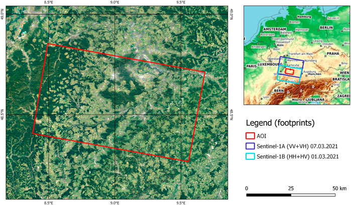
FIGURE 1. Location of the study area (AOI) and extent of the satellite image products. Base map © European Union, contains modified Copernicus data [2022], processed by Bundesamt für Kartographie und Geodäsie (BKG).
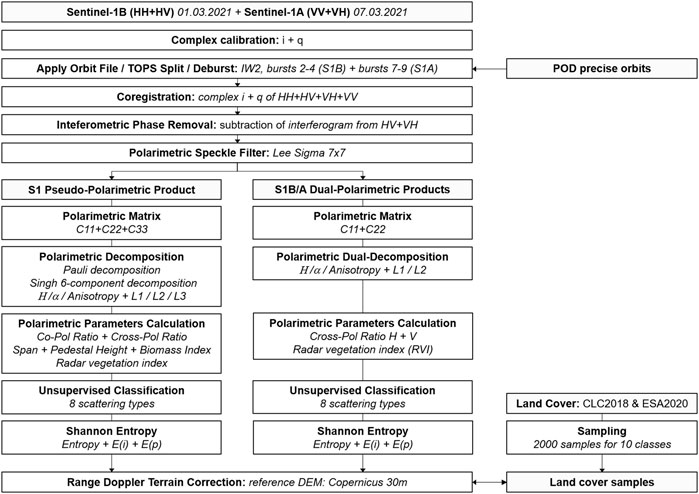
In a first step, the data was radiometrically calibrated with complex output to compensate for different sensitivities in low backscattering areas of Sentinel-1B compared to Sentinel-1A (Schmidt et al., 2020). To increase the geolocation accuracy and the coregistration quality, precise orbit information was retrieved by the Copernicus Precise Orbit Determination (POD) Service (ESA, 2021c) and applied to the metadata. As a consequence of the TOPS (Terrain Observation with Progressive Scan) acquisition mode of Sentinel-1 IW products, portions of an entire image have to be selected (here: sub-swath two; bursts two to four and seven to nine respectively) and merged using the operators “Split” and “Deburst” (Yagüe-Martínez et al., 2016). The resulting subsets cover the same geographic region and were coregistered based on 8,000 randomly generated ground control points (GCPs) which were used to match the two images within a moving registration window having a 32-pixel size, a root mean square error (RMSE) threshold of 0.05, and a cubic interpolation method. A total of 74 GPCs remained after the matching with a mean spatial RMSE of 3.1 m and a standard deviation RMSE of 5.9 m, confirming sub-pixel accuracy. The perpendicular baseline of the images was 126 m. After coregistration using nearest neighbor pixel resampling, the stack contained all four polarizations in their complex representation - real [i] and imaginary [q] parts - which allowed performing polarimetric operators and analyses on the data. To correct for potential errors due to phase difference an interferogram was computed from the HV and VH polarization and subtracted from the data as described by DLR (2006) and Scheiber et al. (2007). The refined Lee Sigma filter was applied to the stack to suppress speckle effects within homogenous areas (Lee et al., 2009). From this step, the synthetic quad-pol information and the original dual-pol products were processed separately as demonstrated in Figure 2.
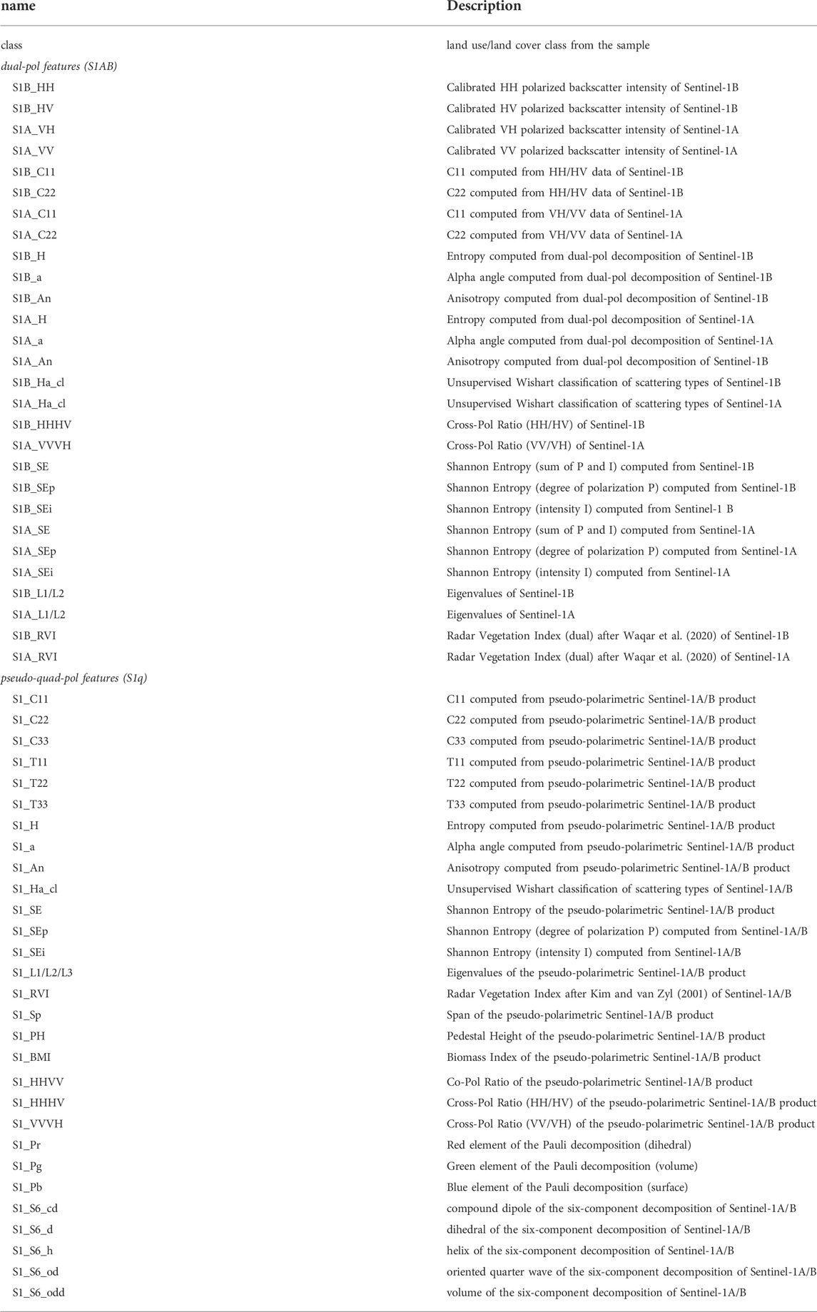
All products were converted to their covariance matrix representations (C3 for quad-pol product, C2 for both Sentinel-1B and Sentinel-1A, respectively) in a first step. Several polarimetric decompositions were applied to the data, including Pauli (Cloude and Pottier, 1996), resulting in surface (blue), dihedral (red), and volume (green) scattering and the model-based six-component decomposition by Singh and Yamaguchi (2018), which furthermore adds helix scattering, oriented dipole scattering and oriented quarter wave reflection to the known three mechanisms. Both decompositions were only applicable to the pseudo-polarimetric stack. Secondly, the eigenvalues of the covariance matrix (L1, L2, L3) were calculated to extract Entropy (H; degree of randomness of targets), Anisotropy (A; impact of secondary scattering mechanism), and the average Alpha angle (α) (Cloude and Pottier, 1996). The same was done for the dual-pol products as proposed by Ji and Wu (2015) for reasons of comparison, although they underline that its application on cross-polarized data, such as Sentinel-1, is of limited quality because of the lack of co-polarization elements. To furthermore increase the polarimetric feature space, different mathematical derivates were calculated, such as the co-pol ratio (HH/VV) and cross-pol-ratio (HH/HV and VV/VH), the span as the summation of the three polarimetric intensity channels (Yahia et al., 2022), the pedestal height as the ratio between minimum and maximum eigenvalue (van Zyl et al., 1987), the Biomass Index (BMI; average co-polarization backscatter intensity), and the Radar Vegetation Index by Kim and van Zyl (2001). None of them were applicable to dual-polarimetric data, except for the RVI under the simplifying assumption that HH and VV are equal (Waqar et al., 2020). Lastly, an unsupervised Wishart classification was conducted resulting in eight physical scattering types based on Entropy and Alpha values (Lee et al., 1999). As especially polarimetric Entropy as described above is barely comparable between the quad-pol and dual-pol inputs, Shannon’s definition of Entropy (E; Shannon, 1948) was additionally computed as the sum of intensity contribution (Ei) and polarimetric contribution (Ep) that depends on the Barakat degree of polarization (Réfrégier et al., 2004). A full list of all available raster variables used in this study is given in Table 1.
All raster datasets were geocoded using Range Doppler terrain correction (Wegmüller, 1999) and the Copernicus World DEM-30 (DLR, 2018) to a final nominal pixel size of 10 m.
2.2 Reference input data
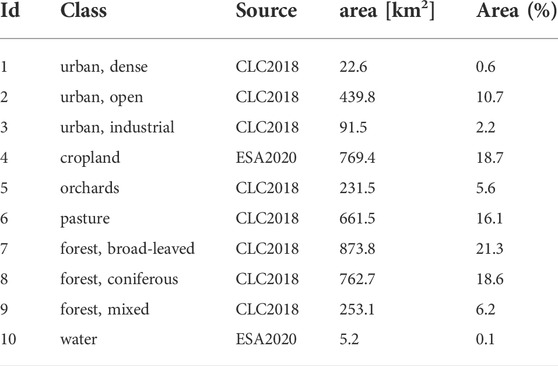
To assess how well the Sentinel-1 pseudo-polarimetric product contributes to the identification and separation of land cover, also in comparison with the standard dual-polarization product, sample points were retrieved from two different datasets which we considered complementary in terms of spatial resolution and class detail. The first one is the ESA World Cover dataset (Zanaga et al., 2021) which contains 11 classes at a spatial resolution of 10 m for the year 2020. It was used for the sampling of water bodies, such as rivers and quarry ponds, as well as agricultural land which is rather small scaled in the study area. However, its class detail was not considered sufficient for this analysis, because it only contains one forest class and one for urban areas. Therefore, the CORINE land cover dataset was used as provided by the European Environment Agency within the Copernicus Programme (EEA, 2020). It has a spatial resolution of 100 m which corresponds to a minimum mapping unit of 25 ha and consists of 44 distinct classes of which 24 occurred within the study area. Classes which were not considered important or which covered very small fractions (e.g. port areas, sport and leisure facilities) were excluded from the analysis. Classes related to urban settlements, cultivated landscapes and different types of forests were retrieved from this dataset. In the end, 2000 samples were randomly generated within each of the ten classes defined in Table 2 and linked to the raster values from Table 1 for an extensive statistical assessment which is presented in the next chapter. The spatial distribution of the samples is shown in Figure 3A.
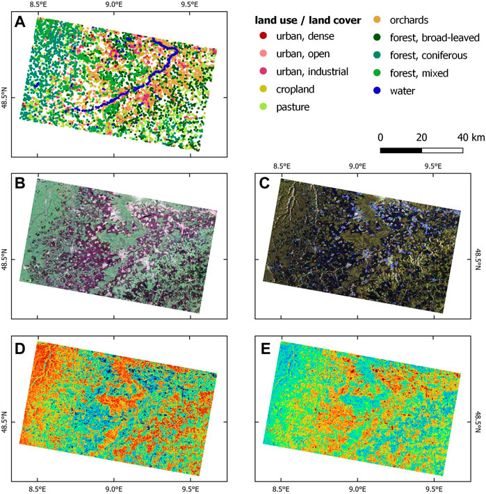
FIGURE 3. (A) land use and land cover samples; (B) Sentinel-1 Pauli decomposition; (C) Sentinel-1 Model-based six-component decomposition (red: oriented dipole, green: helix, blue: oriented quarter wave); (D) Sentinel-1 Entropy (blue to red), (E) Sentinel-1 Anisotropy (blue to red); contains modified Copernicus data [2022].
3 Results
3.1 Visual inspection
Figure 3 shows how the different types of land cover, as represented by the 20,000 samples (A), correspond to the different pseudo-polarimetric features of the Sentinel-1 dataset. The Pauli decomposition (Figure 3B) has the typical signature with single bounce scattering in dark blue, volume scattering in green, and double-bounce scattering in red. Expectedly, the forested areas are characterized by volume scattering of the canopies (green), while cropland, grassland, and barren land produce surface scattering in Sentinel-1’s C-band (blue). The vertical structures of the built-up area in the center (the cities of Tübingen and Reutlingen) produce corner reflection and therefore double bounce returns (red), but the high spatial resolution of Sentinel-1 also allows identifying urban greenspaces within and at the edges of the cities, which are again shown in green. These being visible in the Pauli decomposition demonstrate the successful computation and combination of the four polarizations to construct polarimetric features. Similarly, the model-based six-component decomposition is shown in Figure 3C. Its predominantly dark tones are explainable by fact that oriented dipoles (red), helix scattering (blue) and oriented quarter wave reflection (red) are only making up small proportions of all surfaces. Accordingly, they barely differ for forest and agricultural areas, yet they were found to be complementing the existing basic scattering types (surface, dihedral, volume) in certain cases, especially in man-made environments where they can even be among the dominant scattering mechanisms (Singh and Yamaguchi, 2018). This is confirmed by the different color shadings inside the urban areas which indicate that such polarimetric data allows an even more precise separation morphologic urban structures, for example quarters of different building size or density, as it was already confirmed for dual-pol configurations of Sentinel-1 by Hu et al. (2018).
Lastly, the polarimetric Entropy H and Anisotropy (Figures 3D, E) are shown, representing the degree of randomness or statistical disorder of a target (H) and the impact of secondary scattering mechanism (A), respectively. In this context, a pure target which is totally polarized has a value of H = 0 while a randomly distributed target which is totally unpolarized has a value of H = 1. In Turn, areas which have only one second scattering mechanism behind the dominant one have a high Anisotropy of A = 1 while the value becomes zero when there are several equal secondary scattering mechanisms. Accordingly, forest areas have the highest Entropy values because of the complex scattering behavior of canopies, branches, and leaves, especially along the Carici-Fagetum forest communities of the Jurassic limestone areas of the Swabian Alb (Reif et al., 2017). In turn, urban areas which consist of rather pure targets have low Entropy values which makes them clearly separable from their natural surroundings which are characterized by more distributed targets and therefore medium Entropy (Praks et al., 2009). Complementary to that, the highest Anisotropy values are observed in the agricultural plains and urban areas because these show a high dichotomy of scattering mechanisms which means that both the urban morphology and cropland have a main scattering mechanism followed by a dominant second one (e.g., buildings and paved roads or crops and soil), which is not the case for forest areas (Lee et al., 2008). A statistical analysis of Entropy, Anisotropy and Alpha, especially in relation to the different training classes is given in the next section.
3.2 Statistical evaluation
3.2.1 General statistics and interpretation
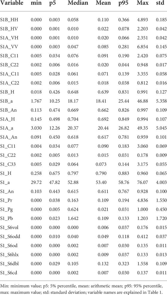
Table 3 lists descriptive statistics of the produced Sentinel-1 bands. It shows that all variables lie within a reasonable range. As expected, the cross-polarization returns (HV and VH) are lower than those of the co-polarization (HH and VV). The table, however, also shows that the calculation of polarimetric features based on two non-coherent images potentially produces values which are not fully covering within the expected range. For instance, the range of the polarimetric Alpha angle (S1_a) is expected to lie between 0 and 90, yet only ranges between 29.7 and 58.8. This will have an impact on the Entropy-Alpha classification of scattering mechanisms, as shown later in this study. At least it reaches higher maxima than those computed from dual-pol data (S1B_a and S1A_a) which range from 1.7 to 49.9 which indicates that high Alpha values are achievable with the proposed method compared to standard Sentinel-1 products.
In a second step, all used variables were tested for correlation. As many of the features are not normal distributed by nature, we calculated Kendall’s Tau (τ) as a rank correlation coefficient which is less prone to outliers (Kendall and Gibbons, 1990). The table is included in the supplementary materials and ranges between +1.0 (strong positive correlation; colored in blue) and -0.879 (strong negative correlation; colored in red). Between all pseudo-polarimetric features, the strongest positive correlations were found between the Pauli elements and the diagonal elements of the Covariance matrix, because of their similar derivation from the cross-polarized elements, above all S1_C22 and the green Pauli element representing volume scattering (τ = 1.0), followed by S1_C11 and the red element (dihedral reflection; τ = 0.683). The high correlation between the second eigenvalues (S1_L2) and volume scattering from the model-based six-component decomposition (S1_6Svol with τ = 0.817) can be explained by its definition as the largest and the smallest eigenvalue sensitive to backscatter intensity (Cloude and Pottier, 1996). The strongest negative correlation between all pseudo-polarimetric features is observed between the pedestal height and the Shannon Entropy (-0.518) which means that they similarly characterize the variety of scattering mechanisms within a pixel, but in a diametrical way. Interestingly, the common scattering types of the two decompositions only show little to no correlation (S1_Pr vs. S1_S6dbl: τ = 0.185; S1_Pg vs. S1_S6vlol: τ = 0.084). This could be attributed to their different derivation and the fact that the latter has larger proportions of three additional scattering types as described above. As expected, Shannon Entropy (S1_SE) and polarimetric Entropy (S1_H) show a low positive correlation with τ = 0.213 which indicates that they refer to a similar concept of statistical disorder, yet they are calculated differently. Looking closer at Shannon Entropy as the sum of two contributions, it is found that its correlation with S1_H is clearly higher for the polarimetric component (S1_Ep with τ = 0.433) compared to the intensity component (S1_Ei with τ = 0.036), which is only related to the total backscattered power (Valle et al., 2013). Accordingly, these correlations indicates that Shannon Entropy and polarimetric Entropy can be considered complementary in the subsequent test for class separability in Section 3.2.3.
With respect to the correlation between the dual-polarization products and the pseudo-polarimetric product, the Kendall correlation analysis shows that there is generally large agreement between the elements of the coherency matrix of the inputs and the generated product with τ = 0.428 for S1B_C11 vs. S1_C33 (HH), τ = 0.525 for S1B_C22 vs. S1_C22 (HV) and τ = 0.960 for S1A_C11 vs. S1_C33 (VV). This is furthermore underlined by the scatter plot between these features in Figure 4. Technically, they originate from the same data, but their differences arise from both resampling of the pixels of the reference product during the coregistration (Section 2.1) and the phase correction described in Section 2.1.
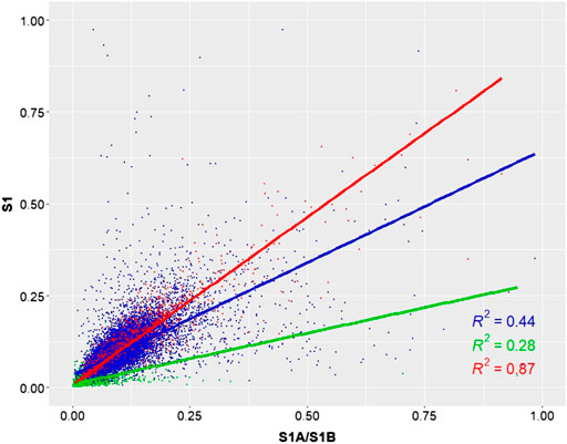
FIGURE 4. Scatter plot between the covariance matrix elements of the pseudo-polarimetric product (y axis) and the dual-polarization inputs (x axis). red: S1A_C11 vs. S1_C33 (VV); green: S1B_C22 vs. S1_C22 (VH); blue S1A_C11 vs. S1_C33 (HH).
Figure 5 shows how well Entropy, Anisotropy and Alpha derived from the pseudo-polarimetric product correlate with those extracted from the dual-polarization data of Sentinel-1A (only VV and VH) as suggested by Ji and Wu (2015). Their correlation measures are confirmed by the scatter plot: The coefficient of determination of R2 = 0.36 states that 36% of the variation observed in the pseudo-polarimetric Entropy (blue, τ = 0.588) can be explained by the entropy derived from the dual-polarization product of Sentinel-1A. A similar relationship is observed for Anisotropy (τ = 0.499 and R2 = 0.36, red), and even a weak negative correlation of τ = -0.152 is observed for the Alpha angle, but only at a very low coefficient of determination of R2 = 0.011 (green). This again underlines that the information gained from pseudo-polarimetric data clearly differ from those retrievable from the standard Sentinel-1 products. We will investigate this difference at more detail in the next section.
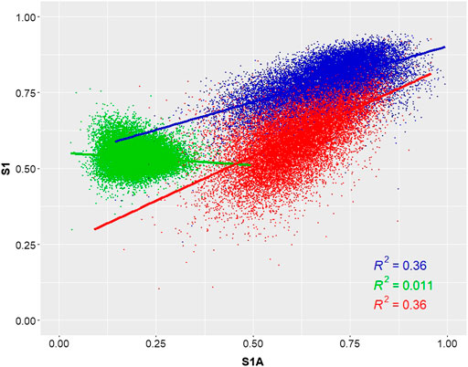
FIGURE 5. Scatter plot between Entropy (blue), Anisotropy (green) and Alpha (red) of the pseudo-polarimetric product (y axis) and the dual-polarization inputs (x axis).
Lastly, we tested how well the Radar Vegetation Index created on dual-polarization data suggested by Waqar et al. (2020) performs with respect to the three scattering mechanisms described by the Pauli decomposition created from the pseudo-polarimetric Sentinel-1 product. To reduce the impact of outliers and non-normal distribution, we converted the Pauli elements to dB scale and created a scatter plot (Figure 6). As expected, both the red (dihedral scattering) and blue (surface scattering) elements are not linearly correlated with the RVI, the green component as an indicator for volume scattering shows a moderate positive correlation of τ = 0.306 with a coefficient of determination of R2 = 0.19. Accordingly, even it was based on only VV and VH in the case of Sentinel-1A, it can partially serve to identify the volume scattering returning from natural surfaces in the study area. As for the RVI calculated from Sentinel-1B (HH and HV), this positive correlation is even slightly higher (τ = 0.417).
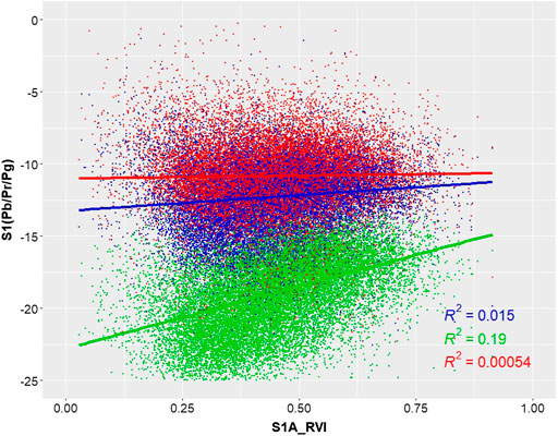
FIGURE 6. Scatter plot between the three Pauli elements of the pseudo-polarimetric product (y axis) and the Radar Vegetation Index computed from dual-polarization Sentinel-1A product. Colors indicate surface (blue), dihedral (red) and volume (green) scattering.
3.2.2 Entropy alpha planes
In this section, the information content of Entropy, Alpha and Anisotropy derived from the pseudo-polarimetric product are tested for their contribution to the identification of different scattering mechanisms, as well as the separation of the observed land use and land cover classes. For this reason, violin plots were created as shown in Figure 7. As indicated in the previous chapter, Entropy (top) is distinctively higher for the three forest classes which have a similar median and a strong concentration of values around it. In comparison, Entropy values of the other classes cover larger but also lower ranges. Especially cropland has the lowest Entropy values because of its rather ordered and structured physical surface characteristics. In contrast to that the Alpha values (middle) are way more similar between the classes and only vary regarding range and standard deviation. Only small proportions of the Alpha values lie outside the range of 45 and 65° which is not uncommon for this parameter, as only areas of strong double bounce or dihedral reflection show high Alpha angles and only in combination with low Entropy values (Cloude and Pottier, 1997). It can be denoted that cropland has the highest range of Alpha values which could be attributed to different degrees of surface roughness on the fields in the study area (DLR, 2006) while broad-leaved forests have the largest concentration of Alpha values at around 55°. As the third parameter, Anisotropy can be considered complementary to Entropy, because it indicates the relative importance of the second and third eigenvalues. It helps to distinguish surfaces especially for Entropies larger than 0.7 because eigenvalues are more prone to SAR system noise at low Entropy (Hajnsek et al., 2003). Accordingly, we expect it to contribute to the separation of the three forest classes in the first term. However, none of the three features shown in Figure 7 alone allows a clear separation of neither forest nor urban classes in the study area. We will test subsequently if their combined use reveals more differences between these classes. As for the orchards which are a typical landscape element of Southern Germany consisting of both meadows and medium-sized trees, their physical properties seem closer to forest areas when looking at Entropy, but in turn, they are more similar to pasture and cropland regarding their Alpha values. Accordingly, this class has a unique polarimetric signature which allows to separate it from its connatural classes.
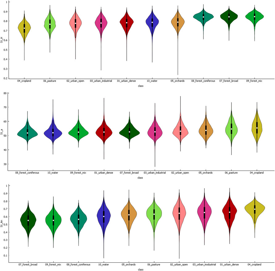
FIGURE 7. Violin plots of Entropy (top), Alpha (middle) and Anisotropy (bottom) for the ten land use and land cover classes. Colors assigned as in Figure 3. Black bars cover the interquartile range (middle 50%) and the white marker indicates the median.
Subsequently, the applicability of the unsupervised Wishart classification is tested by plotting Entropy and Alpha in a coordinate system as proposed by Cloude and Pottier (1997). It is based on the assumption that surfaces can consist of low, moderate, and high Entropy as an indicator of the randomness of scattering inside a pixel, and technically between 0 and 90° regarding their Alpha value, and thereby fall within one of nine basic zones of typical scattering mechanisms (Figure 8 left; adapted from Lee and Pottier, 2009). At first sight, all pixels fall within the feasible regions as marked by the white plot area which confirms the overall quality of the complex calibration and the subsequent steps data processing as described in Section 2.1. The values of the standard dual-polarimetric product (right) are located slightly lower along the y axis, but fully meeting the criteria by Ji and Wu (2015) who redefined the feasible region for dual-polarization data. The most striking difference between both datasets is that the pseudo-polarimetric product (middle) reaches higher Alpha values throughout all classes compared to the dual-polarimetric Sentinel-1 data (right). This is in accordance with reports of similar studies which attest generally low Alpha values achievable by dual-pol data (Dhar et al., 2011). Additionally, as found by systematic comparisons between dual-pol and quad-pol data by Ji and Wu (2015), medium and low Entropy scattering mechanisms are highly confused for HH/HV configurations. The plots based on pseudo-polarimetric data show the typical distribution inside the valid regions with a concentration of pixels in high Entropy zones of moderate Alpha values throughout all classes. However, as already indicated above, when compared to Entropy-Alpha planes of other studies based on actual quad-pol data (Lee et al., 1999), it is obvious that the pseudo-polarimetric data presented here clearly lacks of low Bragg surfaces (zone 3, low Entropy and low Alpha) and a tendency to overestimate dihedral and double reflection (zones 1 and 4, low and moderate Entropy and high Alpha).

FIGURE 8. Entropy-Alpha plots of Sentinel-1 pseudo-polarimetric (middle) and dual-polarimetric (right) data. Color tone indicates point density.
These observations are confirmed when looking at distinct classes in Figure 9. It shows that none of the classes concentrates within one or two specific zones. In turn all of them seem to have their center of gravity in the moderately high Entropy region (zone 4: double reflection; zone 5: anisotropic particles; zone 6: random surface) which is clearly opposed to our expectations with respect to the physical characteristics of these classes. For instance, we would have expected a dominance of dihedral reflectors (Z1) and double reflection (Z4) for urban areas, but these are largely spread over all Alpha regions. Also, water areas are usually characterized by both low Alpha and low Entropy values (Z3, Bragg surface), but in this study, these are concentrated in the moderately high Alpha and very high Entropy areas which correspond to complex structure (Z7) and random anisotropic scatterers (Z8) which is clearly not the case. A similar observation is made for urban areas which should concentrate in zone 4 because of dense aggregations of localized scattering centers which produce moderate Entropy with low order multiple scattering (Cloude and Pottier, 1997). In turn, urban areas in this study only partially fulfill this assumption. A better agreement between the theoretical and observed distribution is observed for forest areas, which are characterized by diffuse scattering and medium Entropy therefore should largely be assigned to zones five and 8 (random anisotropic scatterers; Papathanassiou et al., 2021), which is the case for our data. However, as all classes show a similar trend regarding the distribution of values inside the Entropy Alpha plane, they must be subject to a systematic error of yet unknown degree which must have been introduced during the processing. Accordingly, their use with respect to the actual definition of the scattering mechanisms linked to the zones is strongly limited. Still, classes inside this two-dimensional plot show slightly different distributions when it comes to the center of gravity and range in x and y direction. For instance, nearly all cropland samples have Entropy values between 0.5 and 0.9 while pasture ranges between 0.65 and 0.95. The fact that they barely differ with respect to Alpha suggests testing other polarimetric features for their contribution to a cleaner class separation. The actual benefit of, among others, Entropy and Alpha derived from Sentinel-1 for land cover classification is furthermore investigated in the next section.
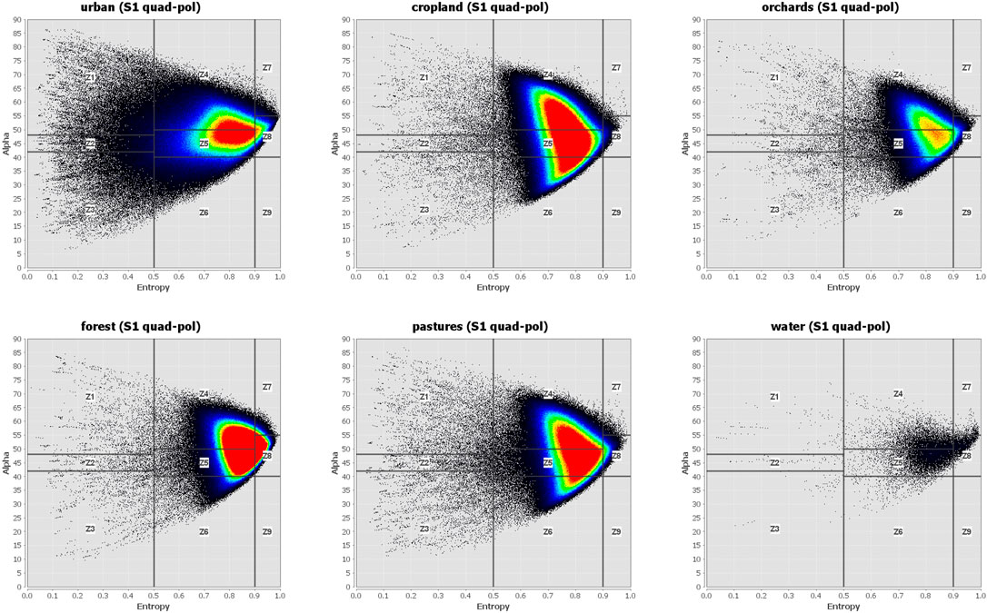
FIGURE 9. Entropy-Alpha plots of selected classes retrieved from Sentinel-1 pseudo-polarimetric data. Forest and urban classes were aggregated for this comparison.
However, as the observed bias related to Alpha values undoubtedly affects the membership of the ten classes, we furthermore reversed this analysis and calculated the proportions of the defined scattering mechanisms over the ten land use and land cover classes. These are shown as stacked bars in Figure 10 and indicate which classes belong to which zone. For instance, double reflection is found among all classes with nearly similar proportion. Random anisotropic scattering (Z8) largely consists of forest areas which is logical as it describes scattering from canopies at high Entropies. The same applies for complex structures (Z7) which is equally distributed over urban and forest classes as both of them contain double-bounce effects, either from trunks or buildings (Singh and Yamaguchi, 2018). Furthermore, dihedral (Z1) and dipole (Z2) reflections are covered by the three urban classes to very large fractions which also is highly feasible due to the presence of as provided by isolated.

FIGURE 10. Distribution of scattering mechanisms based on unsupervised Wishart decomposition over the defined land use and land cover classes in the study area.
Dielectric and metallic dihedral scatterers as well as both double and even bounce effects occur in all urban areas (Cloude and Pottier, 1997). Interestingly, small differences between the urban classes can be observed as the most dominant mechanism in dense urban areas is dipole reflection, while it is complex structures for openly built-up environments and Bragg surfaces (Z3, low Entropy, low Alpha) for industrial areas. However, the latter does not make sense as it should rather cover the water class as discussed above, so this might be part of the bias observed in the Entropy-Alpha plane. In turn, the highest occurrence of water is observed inside the random surface zone (Z6) which is also feasible for rough water bodies, rivers, and coastal areas (Lee et al., 1999). The classes cropland, pasture and orchards show a less distinctive dominance inside one or two zones due to their heterogeneity regarding roughness, structural orders, as well as the size and orientation of the contained vegetation (Voormansik et al., 2016).
3.2.3 Contribution to land cover classification
To test which Sentinel-1 pseudo-polarimetric features are suitable for land cover classification, a feature ranking was performed using the fast correlation-based solution (FCBS) proposed by Yu and Liu (2003). This method identifies the contribution of each variable to the prediction of the target class (here: land use and land cover classes as defined in Table 2) by accounting for redundancies as identified by pairwise variable correlations. According to this ranking, the three most important variables and their respective relative scores are polarimetric Entropy (0.121), Shannon Entropy (0.086) and the co-polarization ratio HH/VV (0.002). This ranking already reveals two things: Firstly, Shannon Entropy as defined by information theory and Entropy as used in SAR polarimetry are highly complementary measures, at least with respect to the samples collected in our study area. Secondly, the comparably low importance of the third feature indicates that many of the variables used in this study (Table 1) are redundant in terms of class separability. This is underlined by the fact that the fourth most important feature was found to be C22 with an importance of 0.00011. In turn, this means that these first three variables already provide a wide feature space to predict the different types of land surfaces. This is visualized by the scatter plot in Figure 11 which shows the land use and land cover classes distributed between a two-dimensional feature space of polarimetric Entropy (x) and Shannon Entropy (y). As it nicely shows, these two variables are more suitable to distinguish between the sampled classes than Entropy and Alpha from the previous section. Forest areas in green tones and urban areas in red tones form clusters in high Shannon Entropy regions whereas cropland, orchards and water bodies are distinguishable in areas of lower Shannon Entropy. Yet, the subdivisions of urban areas and forests do not seem separable based on this projection.
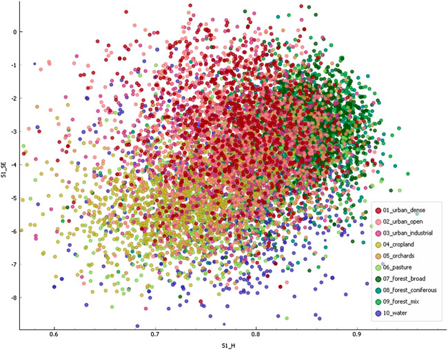
FIGURE 11. Scatter plot between polarimetric Entropy (x) and Shannon Entropy (y) retrieved from Sentinel-1 pseudo-polarimetric data. Colors indicate land use and land cover classes as defined in Table 2.
For this reason, a classification tree was constructed based on all available pseudo-polarimetric variables (Table 1) to test the separability of the three urban classes and the tree forest classes, respectively. A classification tree hierarchically splits the training data based on variable thresholds which are statistically identified by systematic bootstrapping as proposed by Breiman (1996). During this process the training samples are being successively split into subordinated nodes, also called layers, with higher class purity. Constructing classification trees helps to understand the role of variables in a feature set and to identify their most suitable thresholds with respect to the input data’s classification. It has to be noted that increasing the tree depth leads (i.e., using more nodes) leads to a higher prediction accuracy but also makes the tree more complicated and prone to overfitting. As our aim is to understand which of the variables contribute to a clean separation of the classes, we limited the tree depth to four levels. The result is shown in Figure 12. Because the number of classes was limited to three for this test, the variables selected for the most important splits differ from the ones identified by the feature ranking presented above. The most important variable for the urban classes (top) is the blue component of the Pauli decomposition representing surface scattering (S1_Pb, split at 0.101) which mainly divides the input data into openly (left) and densely (right) built-up samples. The left branch is then furthermore divided into open and industrial based on the Alpha angle (S1_a, split at 57.1°). On the right side, the data is split based on the green component of the Pauli decomposition (S1_Pg, split at 0.012) which is interesting because it represents volume scattering which is not a typical component of either of the two classes (dense and industrial). The third level is then based on various variables, including C33, Span, Entropy and the red Pauli component. With these few rules, the tree is already able to correctly predict 40.0% of the 6,000 input training samples, as revealed by an accuracy assessment based on the “leave one out” method - which repeatedly constructs the tree based on the given configuration but leaving out one instance at a time being then classified based on the identified rules. Among all available methods to validate the training accuracy of machine learning classifiers, it is considered one of the most stable but also computationally expensive (Witten, 2011). The outcome of the accuracy assessment is a number referring to the proportion of correctly assigned samples (here: 40% for urban areas) and might seem low at first sight, but it is the product of the three individual classes’ accuracy. If the three single classes are assessed separately, their individual accuracies are 65.3% for dense urban areas, 65.4% for open urban areas and 49.2% for industrial areas. This indicates that large proportions of the observed classes can be separated by the pseudo-polarimetric radar features based on hierarchical splitting. Yet, industrial areas remain hard define by this ruleset, which might be because of either heterogenous physical characteristics inside the defined class, or because of the insufficient spatial resolution of Sentinel-1. Looking at the forest classes, the overall accuracy achieved by the tree classifier is generally lower (39.6%), but widely similar between the three types (broadleaved: 56.5%; coniferous: 59.9%; mixed: 62.8%). Here, the most important variable is C22 (split at 0.024) which already separates large proportions of mixed forest from the other two classes. As this element of the covariance matrix is composed of the two cross-polarizations (HV and VH) it is a suitable descriptor for the different compositions of canopies of broad-leaved and coniferous trees (Lee and Pottier, 2009). Mixed forests are then furthermore refined based on Entropy (S1_H, split at 0.879) and Alpha (S1_a, split at 47.723) which also makes sense from a physical perspective, while on the left side of the tree, the second most important variable is the radar vegetation index (S1_RVI, split at 0.0025) to separate coniferous forests (low RVI) from broadleaved plots (high RVI).
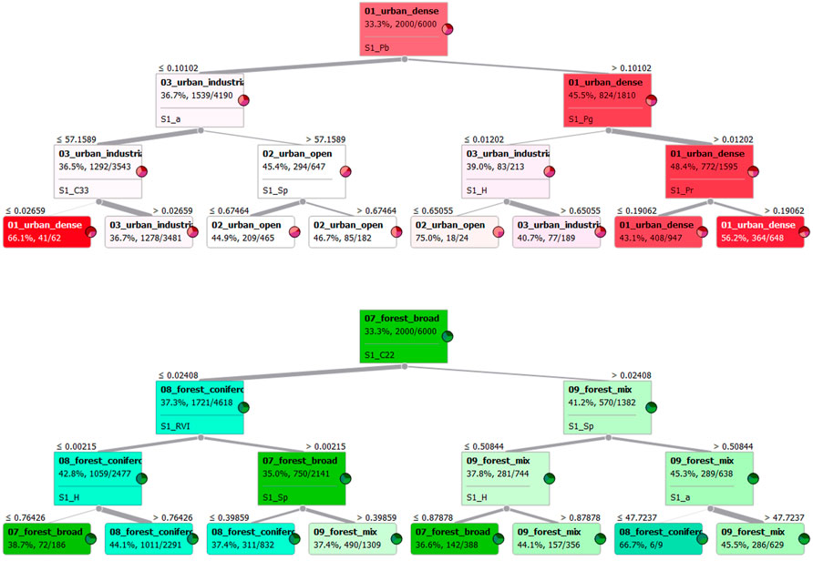
FIGURE 12. Classification trees of urban (top) and forest (bottom) classes based on all available pseudo-polarimetric variables (Table 1). Each node represents a subset of training samples from the level above which are split by the most impactful variable and threshold. Color tones and pie charts indicate class composition and pureness.
Generally, the class prediction accuracy of forest areas is about 10% lower than the one of urban areas which means that the pseudo-polarimetric features calculated in this study have a higher relevance and contribution to the classification of inner-urban areas as compared to woodland. One could assume that increasing the number of layers, and thereby adding more thresholds to split the training data, would furthermore increase the accuracy of the classification trees’ rulesets. However, as already indicated above, this is not always the case, because a considerable proportion of samples is already misclassified at early steps and cannot be separated from other classes at lower levels. This is a known problematic for decision trees (Quinlan, 1986) and visualized in Figure 13. It shows the overall classification accuracy of the trees for all classes (black), as well as for only forest (green) and urban (red) areas. As clearly demonstrated by the black line: if the number of classes is too high, the classification accuracy can no longer be improved by increasing the tree’s depth. Instead, the accuracy starts to go down after six layers due to the problem of overfitting mentioned above. A similar behavior is observed for the accuracy of forest classes which increases by around 2.5 between one and three tree layers but then begins to slightly decrease. Only for the urban classes the accuracy steadily increases from 48.1 to 57.8% before the overfitting causes a decline. Accordingly, tree classifiers are a suitable and transparent method to understand the contribution of features with respect to a target variable, but not a very effective one when it comes to the highest possible classification.
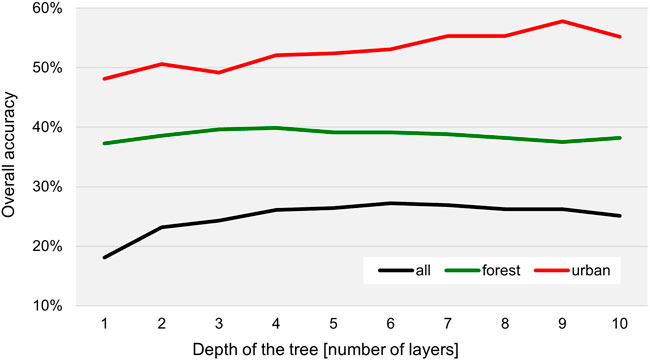
FIGURE 13. Overall accuracies of the classification trees for all ten input classes (black), three forest classes (green) and three urban classes (red) with respect to the number of layers of the constructed decision trees.
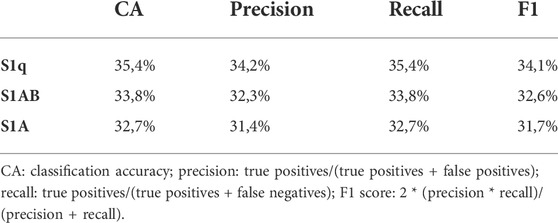
To test how well the data produced in this study is actually suitable to separate the observed classes of land use and land cover, a random forest classifier is used. It is based on the algorithms of classification trees, but adds the component of ensemble learning by repeatedly constructing decision trees based on a random subset of both the explanatory variables (here: raster data Table 1) and their values (Breiman, 2001). This systematically improves the selection of suitable features and increases the robustness of the finally derived value thresholds. In this study, random forests were calculated for both the pseudo-polarimetric parameters (n = 29 [S1q]) as well as for the dual-polarization products (n = 15 for Sentinel-1A only [S1A], n = 30 for both Sentinel-1A and Sentinel-1B [S1AB]) to test for the actual difference regarding their predictive power of the land use and land cover samples. For each of these three settings (S1q, S1A S1AB), 100 trees were calculated, each based on five randomly selected variables, to construct a final complex ruleset to predict the membership of each of the 20,000 training samples to one of the ten defined classes. These rulesets can no longer be visualized as in Figure 12, because they include summarize the decisions of 100 individual trees, but the results is expressed as the classes selected by the majority of trees (Ho, 1998). To evaluate the performance of the trees, which is defined as the suitability to assign the correct class to each of the input samples, a tenfold cross validation was conducted which randomly splits the data into 90% used for training and 10% used for testing ten times to compute the average performance of the classifier (Allen, 1974). Accordingly, the outcome of the validation is the proportion of samples correctly assigned by the random forest. This was done for all classes in total, but also for each class individually to understand which of them are well described by the radar imagery and which are rather complicated to separate from the other classes. The result is shown in Table 4 which lists the classification accuracy (CA) for all classes based on the pseudo-polarimetric data (S1q), the single layers of both input images (S1AB) as well as for the standard Sentinel-1A image containing only VV and VH polarization (S1A). As classification accuracy alone can be a misleading measure, it is complemented by additional statistics: ‘Precision’ connotes the fraction of false positives (falsely assigned samples) and therefore decreases with overestimation of a class, while ‘recall’ is a measure relating completeness which is comprised of the fraction of true positives (correctly assigned samples) compared to true positives and false negatives (missed samples) of a class. Accordingly, recall decreases with underestimation of a class. The F1 score is considered a harmonic mean of precision and recall.
As the table shows, the overall classification accuracy is higher for the pseudo-polarimetric data as compared to the dual-polarization input (S1AB) with clearly higher precision (less falsely assigned classes) but at comparable recall. This indicates that the polarimetric parameters are more effective to classify the land use and land cover classes than the sum of their original inputs. Yet, it has to be denoted that tree classifiers are generally sensitive towards redundancies in data. As showed earlier in Section 3.2.1, much of the variables of Sentinel-1A and Sentinel-1B are highly correlated which can lead to less effective variable selection in the process of tree construction (Quinlan, 1986) and also partly explain the lower accuracies of S1AB compared to S1q. We see the polarimetric parameters of S1q less redundant and therefore more suitable for an ideal exploitation of the inherent information. As expected, the S1A input with only n = 15 variables achieved lower scores than both input images together (S1AB; n = 30) which can be attributed to the smaller population of variables available to identify the best split at the various nodes. Yet, as all of the shown measures are the product of the ten classes’ individual scores, a general conclusion on the superiority of pseudo-polarimetric data cannot be drawn based on Table 4 alone. Therefore, a closer look will be given to the accuracies of each class in Figure 14. It shows that for the majority of land use and land cover classes the prediction accuracy is largest with the pseudo-polarimetric data as input. The strongest increase is observed for pasture with 87.6% compared to the other two datasets with 86.2% (S1AB) and S1A (85.8%). The same is the case for the three urban classes but with slightly less dominance and a generally lower accuracy of industrial areas as observed above. Interestingly, cropland is classified best based on the 30 original bands from the two Sentinel-1 products and even better with data of Sentinel-1A alone than compared with the pseudo-polarimetric data. The same is the case for coniferous forest, but at a slightly lower level, while accuracies of broad-leaved and mixed forests benefit from the polarimetric information. The water class which is generally the one with the highest scores barely shows any accuracy differences because it is the one with the most distinct physical characteristics as compared to the other classes and thereby equally separable regardless of the input data.
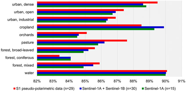
FIGURE 14. Figure 13: Overall accuracies of the random forest classifier based on the pseudo-polarimetric product (red), both Sentinel-1 images (blue) and Sentinel-1A data (green).
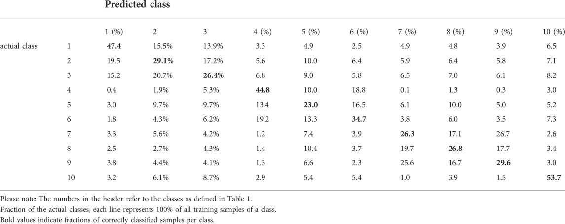
Still, Figure 14 does not explain why certain classes are predicted at a given accuracy and which other classes cause potential mismatch. We have therefore computed an error matrix presented in Table 5 which compares the predictions by the random forest classifier based on of all training samples (columns) with the actual classes of the samples which were fed into the training process (rows). It therefore evaluates, how well the rulesets retrieved from techniques of machine learning are able to separate the observed classes in the study area. It therefore highlights misclassifications between two or more variables which are difficult to separate. As expected, the urban classes share large proportions of confusion among themselves while they are generally well separated from the natural land cover classes. Only the industrial class (3) shares considerable mismatch with the orchards (5) with an overestimation of 9.7% and an underestimation of another 9.0% at the same time which leads to the lowest overall accuracy among the three urban classes. This could be explained by the generally more open morphology of such areas with partly vegetated surfaces. A similar cluster is found for the three forest classes with a strong confusion of around 25% in both directions between broad-leaved (7) and mixed forests (9). As already identified by the decision trees in Figure 12, this class confusion originates from the definition of these classes and the fact that mixed forests partially contain broad-leaved and deciduous forests already. Lastly, the error matrix shows that a considerable amount of misclassification occurs between cropland (4) and pasture (6). For instance, around 19% of the samples predicted as cropland are actually pasture and vice versa. This comes along with findings of other studies which report greater confusion between these classes for C-band pixel-based classifications (Orlikova and Horak, 2019; Borlaf-Mena et al., 2021; Samrat et al., 2021).
Lastly, to analyze how much the input dataset really impacts the classification accuracy, we plotted Receiver Operator Characteristics (ROC) curves of both the pseudo-polarimetric data and the standard Sentinel-1 products for selected classes in Figure 15. ROC are commonly used for the evaluation of machine learning-based outcomes as they plot the false positive rate on their x axis and the true positive rate on the y axis. Accordingly, the closer the plotted curve follows the left-hand and top border, the more accurate the classifier (Davis and Goadrich, 2006). The diagonal line represents a fully random classification outcome. To visually compare the performance of the classifiers under different input datasets, we plotted the scores of the pseudo-polarimetric data (S1q) in dark tones (according to the general colors used in Figure 3) and those of the dual-polarimetric Sentinel-1 images (S1AB) in brighter tones. Firstly, the curves visually underline what is already known from Figure 14, namely that industrial areas, pasture, orchards and coniferous forests are of lower accuracy as visible by their flatter curves. Secondly, classes with higher accuracies, such as densely built-up urban areas, cropland and water, only barely differ regarding the input datasets as both curves are almost identical. The overperformance of S1AB for cropland is visible by the bright yellow line as compared to the darker one. Thirdly, real differences between the input data are only visible for industrial areas, pasture and orchards where S1q outperforms the other input dataset. However, as shown by this analysis, the differences are not as pronounced as maybe implied by the graphs in Figure 14 so that we conclude that the pseudo-polarimetric data does bring benefits for most classes, but not in a significant manner.
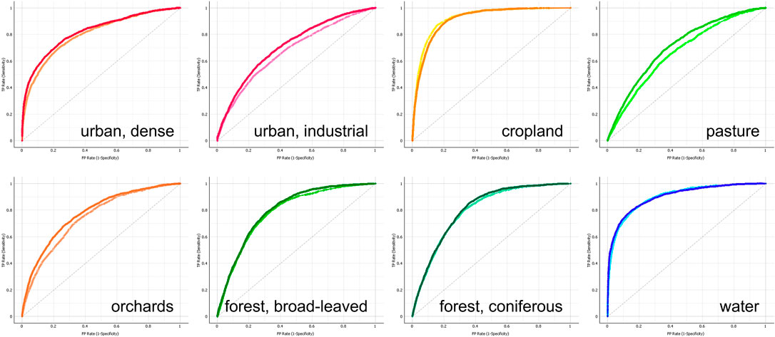
FIGURE 15. Receiver Operator Characteristic (ROC) curves selected land use and land cover classes. Dark tones represent the pseudo-polarimetric input data (S1q) and bright tones the dual-polarimetric products (S1AB).
4 Discussion, conclusion, and outlook
This study tested, on an experimental base, how complementary polarimetric channels of Sentinel-1 data of two different acquisitions can be combined to synthesize a pseudo-polarimetric radar image product. It was performed aware of the fact that such a product cannot fully replace an actual quad-pol acquisition because the two images were acquired at two different dates. As polarimetric analyses are usually performed on the real and imaginary parts of the four polarizations, the scattering integrity of a pixel in terms of coherent scattering of a target cannot be assured by this approach, thus leading to the observed differences in decomposition elements or Entropy, for instance. Yet, the findings show that the information content of Sentinel-1 data is largely comparable to actual quad-pol data that polarimetric derivates have a positive impact on land cover classifications compared to pure backscatter intensity of the four polarizations. The following paragraphs will discuss open points and put the results into perspective regarding how future studies could benefit from the findings of this work.
From the processing point of view, it is questionable if combining two images with complementary polarization bands can simply be coregistered to form a quad-pol product. Besides the obvious flaws at the theoretical level outlined in the previous paragraph, it was highlighted in Section 3.2.2 that, despite complex calibration and phase correction, there is bias inherent to the data. This indicates that also other polarimetric parameters are potentially subject to that bias. It should therefore be tested in further studies how the four bands could be radiometrically calibrated in terms of channel imbalance or cross-talk, for example, by analyzing the returns of all four polarizations from trihedral corner reflectors (van Zyl, 1990). Besides this polarimetric calibration, methods of incidence angle normalization should be considered in areas of strong topography, as suggested by Atwood et al. (2012) who report an improvement in classification accuracy by 15% using a radiometric terrain correction of the polarimetric input product. As shown in Figure 3, especially the model-based six-component decomposition and Entropy are strongly affected by deep valleys ranging in north-south direction in the northwest region as with the many ridges of the Swabian Alb in the southeastern center of the study area.
Another apparent source of error is the fact that Sentinel-1 imagery of complementary polarimetric information was only available from the year 2021 while the land cover classifications are from 2018 to 2020. Accordingly, a small proportion of pixels could underlie a mismatch between the actual surface as observed by Sentinel-1 and the one expected by the reference data. Furthermore, the spatial resolution of CLC2018 was 100 m which means that some of the randomly sampled pixels could have been falsely assigned at the borders of classes and inside small pixel groups. Based on the sample size of 2000 per class, we consider the effect of temporal and spatial integrity on the quality of the results statistically small. The same applies for the slightly different incidence angle (39.05° for S1B and 39.10° for S1A at mid-swath) which can potentially lead to different returns among the different bands, as indicated by Stiles et al. (2000) who report a general dependence of polarimetric signatures over grasslands from the incidence angle of the system.
The visual inspection of polarimetric radar products of Sentinel-1 (Figure 3) shows that the overall information content is as expected. Yet, a regular striping effect was observed which might have been caused by the coregistration of Sentinel-1A and Sentinel-1B which introduced linear patterns in north-south directions for the polarimetric decompositions and in east-west direction for Entropy and Alpha. We tried different resampling options (nearest neighbor, bilinear, bicubic) and transformations of the coregistered product, but could not fully eliminate these systematic patterns. Still, we believe that their impact on the results and their interpretation is insignificant.
The presented visual inspection of the Entropy Alpha planes leads to the conclusion that the distribution of the pseudo-polarimetric data is only partly logical and feasible, but still of higher information content than the standard dual-polarization product of Sentinel-1. However, several observations indicate that the potential of an unsupervised Wishart classification based on pseudo-polarimetric Sentinel-1 features is biased and cannot fully be exploited, especially when it comes to the assignment of physical properties. It should therefore be interpreted with care. As it turned out, class assignment based on methods of machine learning were more effective than traditional Entropy-Alpha decomposition, although these polarimetric measures revealed a systematic dependence from the sampled land use and land cover classes (Figure 7).
Different from working with calibrated optical imagery, our statistical analysis showed that the different variables used in this study strongly vary regarding range and standard deviation (Table 3) and only few of them are normal distributed. This requires the application of classifiers which are based on thresholds rather than on cluster centers or bounding boxes. We therefore selected the classification tree and random forest classifiers. The classification tree based on random samples of all ten land cover classes showed that the main elements of the landscape were well delineable by the Sentinel-1 polarimetric bands. It furthermore showed that a sufficient degree of class separation was already achievable with the four highest ranked variables (Entropy, Shannon Entropy, co-polarization ratio, and C22). Within this context, polarimetric features turned out to have a bigger impact than the pure co-pol or cross-pol backscatter intensities. Surely, higher accuracies could have been achieved by the integration of more elaborated classifiers, such as Support Vector Machines (Rahman et al., 2020) or segmentation-based approaches using Convolutional Neural Networks (Hoeser et al., 2020). However, the main goal in this study was to identify which variables derived from Sentinel-1 are most relevant and which value thresholds based on C-band signatures allow a best possible class discrimination within a transparent process. The tree classifier has proven effective for this cause, but it requires either a preceding feature ranking to restrict the creation of the tree to a small number of input bands, or the definition of a maximum tree depth to avoid overfitting. Furthermore, it reaches its limits when applied to a large number of classes, as demonstrated in Figure 13. The advancement of these binary decision tree concepts in form of a ensemble-based random forest classifier showed that higher classification accuracies are possible, but too many misclassifications exist between similar classes, such as cropland and pasture or—to our surprise—industrial areas and orchards. These could maybe reduced by applying Gradient Boosting classifiers which operate based on similar ensemble principles as random forests but are reported to outperform them in terms of classification accuracy (Lin et al., 2014; Sahin, 2020). In this study, we only evaluated the training accuracy of these classifiers based on an extensive set of class samples. Yet, for actual image classifications which aim at the best possible prediction of land use and land cover based on sparsely available training data, more emphasis should be placed on the role and preprocessing of the selected input variables and an actual validation should be performed using data independently collected for testing. A classic analysis would also include a more careful selection of classes. We found that some of the classes used in our study were strongly related to land use (e.g. industrial) and not really physical representation of the Earth’s surface. In this context, the class “mixed forest” turned out to decrease the overall accuracy because it physically consisted of the two other classes (broad-leaved and coniferous). Accordingly, for SAR-based approaches, class definitions should be clear and non-overlapping.
Finally, when comparing results from the pseudo-polarimetric product synthesized in this study and its two dual-polarization input products, we found that the overall differences regarding classification accuracy are rather subtle and refrained to certain classes. In our case, dense urban areas, pasture and mixed forest profited the most from the computation of the pseudo-polarimetric features as input for the classification. Although this effect was not observed for all classes, we found the polarimetric features less redundant and therefore more suitable for an ideal exploitation of the inherent information. Yet, while a general superiority of pseudo-polarimetric could be assumed from the by the data, the actual improvement in classification accuracy only ranges between 0.1% (water) and 1.8% (pasture). It is to be tested in further studies if the suggested approach brings greater benefit for the discrimination of particular land cover types, such as savanna ecosystems of different tree density, mangroves in coastal zones, or wetlands with vegetation gradients.
Although the availability of data from Sentinel-1B is no longer given (Brainard, 2022; ESA, 2022), we see potential in the provided research to assist the design of the upcoming launches of Sentinel-1C and Sentinel-1D in such a way that these will deliver complementary polarimetric information at repeat intervals of three to 6 days within a relative orbit (Torres et al., 2021). The findings in this study show that combining two products of short temporal baseline can not only contribute to interferometric analyses but also increase the polarimetric mapping capabilities of the entire mission.
Data availability statement
The datasets used in this study are provided by the European Space Agency within the Copernicus Programme and can be downloaded at: https://scihub.copernicus.eu/dhus. The following products were used: S1B_IW_SLC__1SDH_20210301T053409_20210301T053433_025817_03141E_C422, S1A_IW_SLC__1SDV_20210307T053437_20210307T053505_036888_0456B1_EF47.
Author contributions
AB was responsible for the research design and conception and data processing. EO contributed in creation of the figures and parts of the statistical analysis. Both authors have written, read, and approved the submitted manuscript and actively engaged in the peer-review process.
Funding
This study was partially funded within the Christian Doppler Laboratory for Geospatial and EO-based Humanitarian Technologies (GeoHum) with support from the Christian Doppler Research Association and Médecins Sans Frontières (MSF) Austria. Sentinel-1 data was provided by the European Space Agency (ESA) within the Copernicus Programme.
Acknowledgments
We thank Edward Cahill for proofreading the manuscript and the numerous developers of open-source software for geospatial data processing, among others ESA SNAP (especially Jun Lu for his valuable comments on polarimetric stack generation), PolSAR Pro and Orange Data Mining.
Conflict of interest
The authors declare that the research was conducted in the absence of any commercial or financial relationships that could be construed as a potential conflict of interest.
Publisher’s note
All claims expressed in this article are solely those of the authors and do not necessarily represent those of their affiliated organizations, or those of the publisher, the editors and the reviewers. Any product that may be evaluated in this article, or claim that may be made by its manufacturer, is not guaranteed or endorsed by the publisher.
Supplementary material
The Supplementary Material for this article can be found online at: https://www.frontiersin.org/articles/10.3389/frsen.2022.905713/full#supplementary-material
References
Allen, D. M. (1974). The relationship between variable selection and data agumentation and a method for prediction. Technometrics 16, 125–127. doi:10.1080/00401706.1974.10489157
Atwood, D. K., Small, D., and Gens, R. (2012). Improving PolSAR land cover classification with radiometric correction of the coherency matrix. IEEE J. Sel. Top. Appl. Earth Obs. Remote Sens. 5, 848–856. doi:10.1109/JSTARS.2012.2186791
Bhogapurapu, N., Dey, S., Bhattacharya, A., Mandal, D., Lopez-Sanchez, J. M., McNairn, H., et al. (2021). Dual-polarimetric descriptors from Sentinel-1 GRD SAR data for crop growth assessment. ISPRS J. Photogrammetry Remote Sens. 178, 20–35. doi:10.1016/j.isprsjprs.2021.05.013
Borlaf-Mena, I., Badea, O., and Tanase, M. A. (2021). “Influence of the mosaicking algorithm on sentinel-1 land cover classification over rough terrain,” in International Geoscience and Remote Sensing Symposium (IEEE), 6646–6649.
Brainard, J. (2022). News at a glance: Orbiting radar mapper goes dark. Science 375, 700–702. doi:10.1126/science.ada1329
Braun, A., Fakhri, F., and Hochschild, V. (2019). Refugee camp monitoring and environmental change assessment of Kutupalong, Bangladesh, based on radar imagery of sentinel-1 and ALOS-2. Remote Sens. 11, 2047. doi:10.3390/rs11172047
D. Closson, N. Milisavljevic, P. Pasquali, and F. Holecz (Editors) (2014). Land applications of radar remote sensing (Rijeka, Croatia: IntechOpen).
Cloude, S. R., and Pottier, E. (1996). A review of target decomposition theorems in radar polarimetry. IEEE Trans. Geosci. Remote Sens. 34, 498–518. doi:10.1109/36.485127
Cloude, S. R., and Pottier, E. (1997). An entropy based classification scheme for land applications of polarimetric SAR. IEEE Trans. Geosci. Remote Sens. 35, 68–78. doi:10.1109/36.551935
Davis, J., and Goadrich, M. (2006). “The relationship between Precision-Recall and ROC curves,” in Proceedings of the 23rd international conference on machine learning. Editors W. Cohen, and A. Moore (New York: ACM Press), 233–240.
Dhar, A. T., Gray, B. D., and Menges, C. C. (2011). “Comparison of dual and full polarimetric entropy/alpha decompositions with TerraSAR-X, suitability for use in classification,” in 2011 IEEE International Geoscience and Remote Sensing Symposium: (IGARSS 2011), Vancouver, BC, Canada, 24 - 29 July 2011 (Piscataway, NJ: IEEE), 456–458. [proceedings.
DLR (2006). AgriSAR: Agricultural bio-/geophysical Retrievals from frequent repeat SAR and optical imaging. Final report. Available at: https://earth.esa.int/eogateway/campaigns/agrisar-2006 (Accessed August 15, 2022).
EEA (2020). Corine land cover (CLC) 2018: Version 2020_20u1. Available at: https://land.copernicus.eu/pan-european/corine-land-cover/clc2018 (Accessed May 15, 2020).
ESA (2021a). Copernicus sentinel-1 calibration campaign on-going in europe: 12 january 2021. Available at: https://sentinel.esa.int/web/sentinel/-/copernicus-sentinel-1-calibration-campaign-on-going-in-europe (Accessed November 01, 2021).
ESA (2022). Mission ends for Copernicus sentinel-1B satellite. Available at: https://www.esa.int/Applications/Observing_the_Earth/Copernicus/Sentinel-1/Mission_ends_for_Copernicus_Sentinel-1B_satellite (Accessed August 15, 2022).
ESA (2021b). Sentinel-1 SAR: Level-1 interferometric wide swath SLC products. Available at: https://sentinels.copernicus.eu/web/sentinel/technical-guides/sentinel-1-sar/products-algorithms/level-1/single-look-complex/interferometric-wide-swath (Accessed November 01, 2021).
ESA (2021d). Snap - ESA sentinel application Platform v. 8.0.5. Available at: http://step.esa.int.
Hajnsek, I., Pottier, E., and Cloude, S. R. (2003). Inversion of surface parameters from polarimetric SAR. IEEE Trans. Geosci. Remote Sens. 41, 727–744. doi:10.1109/TGRS.2003.810702
Haldar, D., Verma, A., Kumar, S., and Chauhan, P. (2021). Estimation of mustard and wheat phenology using multi-date Shannon entropy and Radar Vegetation Index from polarimetric Sentinel- 1. Geocarto Int. 37, 5935–5962. doi:10.1080/10106049.2021.1926554
Herzog, F. (1998). Streuobst: A traditional agroforestry system as a model for agroforestry development in temperate europe. Agrofor. Syst. 42, 61–80. doi:10.1023/A:1006152127824
Ho, T. K. (1998). The random subspace method for constructing decision forests. IEEE Trans. Pattern Anal. Mach. Intell. 20, 832–844. doi:10.1109/34.709601
Hoeser, T., Bachofer, F., and Kuenzer, C. (2020). Object detection and image segmentation with deep learning on Earth observation data: A review—Part II: Applications. Remote Sens. 12, 3053. doi:10.3390/rs12183053
Hu, J., Ghamisi, P., and Zhu, X. (2018). Feature extraction and selection of sentinel-1 dual-pol data for global-scale local climate zone classification. ISPRS Int. J. Geoinf. 7, 379. doi:10.3390/ijgi7090379
Ji, K., and Wu, Y. (2015). Scattering mechanism extraction by a modified cloude-pottier decomposition for dual polarization SAR. Remote Sens. 7, 7447–7470. doi:10.3390/rs70607447
Jo, M. J., Osmanoglu, B., Zhang, B., and Wdowinski, S. (2018). Flood extent mapping using dual-polarimetric Sentinel-1 synthetic aperture radar imagery. Int. Arch. Photogramm. Remote Sens. Spat. Inf. Sci. 42, 711–713. doi:10.5194/isprs-archives-xlii-3-711-2018
Jutz, S., and Milagro-Pérez, M. P. (2020). Copernicus: The European Earth observation programme. Rev. Teledetec. doi:10.4995/raet.2020.14346
Kim, Y., and van Zyl, J. (2001). “Comparison of forest parameter estimation techniques using SAR data,” in IEEE 2001 international geoscience and remote sensing symposium (IEEE), 1395–1397.
Lee, J.-S., Ainsworth, T. L., Kelly, J. P., and Lopez-Martinez, C. (2008). Evaluation and bias removal of multilook effect on entropy/alpha/anisotropy in polarimetric SAR decomposition. IEEE Trans. Geosci. Remote Sens. 46, 3039–3052. doi:10.1109/TGRS.2008.922033
Lee, J.-S., Grunes, M. R., Ainsworth, T. L., Li-Jen, D, Schuler, D. L., and Cloude, S. R. (1999). Unsupervised classification using polarimetric decomposition and the complex Wishart classifier. IEEE Trans. Geosci. Remote Sens. 37, 2249–2258. doi:10.1109/36.789621
Lee, J.-S., and Pottier, E. (2009). Polarimetric radar imaging: From basics to applications. Boca Raton, Fla: CRC Press/Taylor & Francis.
Lee, J.-S., Wen, J.-H., Ainsworth, T. L., Chen, K.-S., and Chen, A. J. (2009). Improved Sigma filter for speckle filtering of SAR imagery. IEEE Trans. Geosci. Remote Sens. 47, 202–213. doi:10.1109/tgrs.2008.2002881
Lin, L., Yue, W., and Mao, Y. (2014). Multi-class image classification based on fast stochastic gradient boosting. Informatica 28, 145–153.
Lu, Y., Yang, C., and Meng, Z. (2021). Lithology discrimination using sentinel-1 dual-pol data and SRTM data. Remote Sens. 13, 1280. doi:10.3390/rs13071280
Mandal, D., Kumar, V., Ratha, D., Dey, S., Bhattacharya, A., Lopez-Sanchez, J. M., et al. (2020). Dual polarimetric radar vegetation index for crop growth monitoring using Sentinel-1 SAR data. Remote Sens. Environ. 247, 111954. doi:10.1016/j.rse.2020.111954
Mascolo, L., Cloude, S. R., and Lopez-Sanchez, J. M. (2022). Model-based decomposition of dual-pol SAR data: Application to sentinel-1. IEEE Trans. Geosci. Remote Sens. 60, 1–19. doi:10.1109/TGRS.2021.3137588
Nasirzadehdizaji, R., Balik Sanli, F., Abdikan, S., Cakir, Z., Sekertekin, A., and Ustuner, M. (2019). Sensitivity analysis of multi-temporal sentinel-1 SAR parameters to crop height and canopy coverage. Appl. Sci. 9, 655. doi:10.3390/app9040655
Nguyen, H. H., Cho, S., Jeong, J., and Choi, M. (2021). A D-vine copula quantile regression approach for soil moisture retrieval from dual polarimetric SAR Sentinel-1 over vegetated terrains. Remote Sens. Environ. 255, 112283. doi:10.1016/j.rse.2021.112283
Orlikova, L., and Horak, J. (2019). “Land cover classification using sentinel-1 SAR data,” in International Conference on Military Technologies (IEEE), 1–5.
Papathanassiou, K. P., Cloude, S. R., Pardini, M., Quiñones, M. J., Hoekman, D., Ferro-Famil, L., et al. (2021). “Forest applications,” in Polarimetric synthetic aperture radar. Editors I. Hajnsek, and Y.-L. Desnos (Cham: Springer International Publishing), 59–117.
Periasamy, S. (2018). Significance of dual polarimetric synthetic aperture radar in biomass retrieval: An attempt on Sentinel-1. Remote Sens. Environ. 217, 537–549. doi:10.1016/j.rse.2018.09.003
Petris, S. d., Sarvia, F., Gullino, M., Tarantino, E., and Borgogno-Mondino, E. (2021). Sentinel-1 polarimetry to map apple orchard damage after a storm. Remote Sens. 13, 1030. doi:10.3390/rs13051030
Plank, S., Jüssi, M., Martinis, S., and Twele, A. (2017). Mapping of flooded vegetation by means of polarimetric Sentinel-1 and ALOS-2/PALSAR-2 imagery. Int. J. Remote Sens. 38, 3831–3850. doi:10.1080/01431161.2017.1306143
Plieninger, T., Bieling, C., Ohnesorge, B., Schaich, H., Schleyer, C., and Wolff, F. (2013). Exploring futures of ecosystem services in cultural landscapes through participatory scenario development in the swabian Alb, Germany. Ecol. Soc. 18, art39. doi:10.5751/ES-05802-180339
Potin, P., Gascon, F., Mecklenburg, S., Zehner, C., and Laur, H. (2019a). Sentinel high level operations plan (HLOP). Available at: https://sentinels.copernicus.eu/documents/247904/685154/Sentinel_High_Level_Operations_Plan.
Potin, P., Rosich, B., Miranda, N., Grimont, P., Shurmer, I., O'Connell, A., et al. (2019b). “Copernicus sentinel-1 constellation mission operations status,” in IEEE 2019 International Geoscience and Remote Sensing Symposium (IEEE), 5385–5388.
Pottier, E., Ferro-Famil, L., Fitrzyk, M., and Desnos, Y. L. (2018). “PolSARpro-BIO: The new scientific toolbox for ESA & third party fully polarimetric SAR missions,” in 12th European conference on synthetic aperture radar.
Praks, J., Koeniguer, E. C., and Hallikainen, M. T. (2009). Alternatives to target entropy and alpha angle in SAR polarimetry. IEEE Trans. Geosci. Remote Sens. 47, 2262–2274. doi:10.1109/TGRS.2009.2013459
Rahman, A., Abdullah, H. M., Tanzir, M. T., Hossain, M. J., Khan, B. M., Miah, M. G., et al. (2020). Performance of different machine learning algorithms on satellite image classification in rural and urban setup. Remote Sens. Appl. Soc. Environ. 20, 100410. doi:10.1016/j.rsase.2020.100410
Réfrégier, P., Goudail, F., Chavel, P., and Friberg, A. (2004). Entropy of partially polarized light and application to statistical processing techniques. J. Opt. Soc. Am. A 21, 2124–2134. doi:10.1364/josaa.21.002124
Reif, A., Xystrakis, F., Gärtner, S., and Sayer, U. (2017). Floristic change at the drought limit of European beech (fagus sylvatica L.) to downy oak (quercus pubescens) forest in the temperate climate of central europe. Not. Bot. Horti Agrobot. Cluj. Napoca. 45, 646–654. doi:10.15835/nbha45210971
Roda Husman, S. de, van der Sanden, J. J., Lhermitte, S., and Eleveld, M. A. (2021). Integrating intensity and context for improved supervised river ice classification from dual-pol Sentinel-1 SAR data. Int. J. Appl. Earth Observation Geoinformation 101, 102359. doi:10.1016/j.jag.2021.102359
Sahin, E. K. (2020). Assessing the predictive capability of ensemble tree methods for landslide susceptibility mapping using XGBoost, gradient boosting machine, and random forest. SN Appl. Sci. 2, 1308. doi:10.1007/s42452-020-3060-1
Samrat, A., Devy, M. S., and Ganesh, T. (2021). Delineating fragmented grassland patches in the tropical region using multi-seasonal synthetic aperture radar (SAR) and optical satellite images. Int. J. Remote Sens. 42, 3938–3954. doi:10.1080/01431161.2021.1881181
Scheiber, R., Keller, M., Fischer, J., Andres, C., Horn, R., and Hajnsek, I. (2007). “Radar data processing, quality analysis and level-1b product generation forAGRISAR and EAGLE campaigns,” in Proceedings of the AGRISAR and EAGLE campaigns final workshop (ESA), 1–8.
Schmidt, K., Schwerdt, M., Miranda, N., and Reimann, J. (2020). Radiometric comparison within the sentinel-1 SAR constellation over a wide backscatter range. Remote Sens. 12, 854. doi:10.3390/rs12050854
Shannon, C. E. (1948). A mathematical theory of communication. Bell Syst. Tech. J. 27, 379–423. doi:10.1002/j.1538-7305.1948.tb01338.x
Singh, G., and Yamaguchi, Y. (2018). Model-based six-component scattering matrix power decomposition. IEEE Trans. Geosci. Remote Sens. 56, 5687–5704. doi:10.1109/tgrs.2018.2824322
Stiles, J. M., Sarabandi, K., and Ulaby, F. T. (2000). Electromagnetic scattering from grassland. II. Measurement and modeling results. IEEE Trans. Geosci. Remote Sens. 38, 349–356. doi:10.1109/36.823930
Torres, R., Lokas, S., Bibby, D., Geudtner, D., Navas-Traver, I., Ceba Vega, F., et al. (2021). 13th European Conference on Synthetic Aperture Radar, 1–4.The sentinel-1C/-1D development and deployment plan
Valle, H. D., Hardke, L., Blanco, P. D., and Sione, W. (2013). Assessment of land degradation using Shannon entropy approach on polsar images in patagonian coastal deserts. GeoFocus 13, 84–111.
van Zyl, J. J. (1990). Calibration of polarimetric radar images using only image parameters and trihedral corner reflector responses. IEEE Trans. Geosci. Remote Sens. 28, 337–348. doi:10.1109/36.54360
van Zyl, J. J., Zebker, H. A., and Elachi, C. (1987). Imaging radar polarization signatures: Theory and observation. Radio Sci. 22, 529–543. doi:10.1029/RS022i004p00529
Varade, D., Maurya, A. K., Dikshit, O., Singh, G., and Manickam, S. (2020). Snow depth in dhundi: An estimate based on weighted bias corrected differential phase observations of dual polarimetric bi-temporal sentinel-1 data. Int. J. Remote Sens. 41, 3031–3053. doi:10.1080/01431161.2019.1698076
Voormansik, K., Jagdhuber, T., Zalite, K., Noorma, M., and Hajnsek, I. (2016). Observations of cutting practices in agricultural grasslands using polarimetric SAR. IEEE J. Sel. Top. Appl. Earth Obs. Remote Sens. 9, 1382–1396. doi:10.1109/JSTARS.2015.2503773
Waqar, M., Sukmawati, R., Ji, Y., and Sri Sumantyo, J. (2020). Tropical PeatLand forest biomass estimation using polarimetric parameters extracted from RadarSAT-2 images. Land 9, 193. doi:10.3390/land9060193
Wegmüller, U. (1999). “Automated terrain corrected SAR geocoding,” in IEEE 1999 International Geoscience and Remote Sensing Symposium (IEEE).
Witten, I. H. (2011). Data mining: Practical machine learning tools and techniques. Burlington, MA: Morgan Kaufmann Publishers.
Xie, L., Zhang, H., Wang, C., and Shan, Z. (2015). Similarity analysis of entropy/alpha decomposition between HH/VV dual- and quad-polarization SAR data. Remote Sens. Lett. 6, 228–237. doi:10.1080/2150704X.2015.1026954
Yagüe-Martínez, N., Prats-Iraola, P., Rodriguez Gonzalez, F., Brcic, R., Shau, R., Geudtner, D., et al. (2016). Interferometric processing of Sentinel-1 TOPS data. IEEE Trans. Geosci. Remote Sens. 54, 2220–2234. doi:10.1109/TGRS.2015.2497902
Yahia, M., Ali, T., and Mortula, M. M. (2022). Span statistics and their impacts on PolSAR applications. IEEE Geosci. Remote Sens. Lett. 19, 1–5. doi:10.1109/LGRS.2020.3039109
Yu, L., and Liu, H. (2003). “Feature selection for high-dimensional data: A fast correlation-based filter solution,” in Proceedings of the Twentieth International Conference on Machine Learning (Menlo Park, California: AAAI Press), 856–863.
Keywords: SAR polarimetry (PolSAR), Sentinel-1, land-cover mapping, ALOS-2, radar polarimetry analysis, synthetic aperture radar
Citation: Braun A and Offermann E (2022) Polarimetric information content of Sentinel-1 for land cover mapping: An experimental case study using quad-pol data synthesized from complementary repeat-pass acquisitions. Front. Remote Sens. 3:905713. doi: 10.3389/frsen.2022.905713
Received: 27 March 2022; Accepted: 31 August 2022;
Published: 28 September 2022.
Edited by:
Paola Rizzoli, German Aerospace Center (DLR), GermanyReviewed by:
Juan M. Lopez-Sanchez, University of Alicante, SpainLachezar Filchev, Space Research and Technology Institute (BAS), Bulgaria
Copyright © 2022 Braun and Offermann. This is an open-access article distributed under the terms of the Creative Commons Attribution License (CC BY). The use, distribution or reproduction in other forums is permitted, provided the original author(s) and the copyright owner(s) are credited and that the original publication in this journal is cited, in accordance with accepted academic practice. No use, distribution or reproduction is permitted which does not comply with these terms.
*Correspondence: Andreas Braun, YW4uYnJhdW5AdW5pLXR1ZWJpbmdlbi5kZQ==
 Andreas Braun
 Eric Offermann1