Hybrid Semi-Analytical Algorithm for Estimating Chlorophyll-A Concentration in Lower Amazon Floodplain Waters

The Amazon Basin is the largest on the planet, and its aquatic ecosystems affect and are affected by the Earth’s processes. Specifically, Amazon aquatic ecosystems have been subjected to severe anthropogenic impacts due to deforestation, mining, dam construction, and widespread agribusiness expansion. Therefore, the monitoring of these impacts has become crucial for conservation plans and environmental legislation enforcement. However, its continental dimensions, the high variability of Amazonian water mass constituents, and cloud cover frequency impose a challenge for developing accurate satellite algorithms for water quality retrieval such as chlorophyll-a concentration (Chl-a), which is a proxy for the trophic state. This study presents the first application of the hybrid semi-analytical algorithm (HSAA) for Chl-a retrieval using a Sentinel-3 OLCI sensor over five Amazonian floodplain lakes. Inherent and apparent optical properties (IOPs and AOPs), as well as limnological data, were collected at 94 sampling stations during four field campaigns along hydrological years spanning from 2015 to 2017 and used to parameterize the hybrid SAA to retrieve Chl-a in highly turbid Amazonian waters. We implemented a re-parametrizing approach, called the generalized stacked constraints model to the Amazonian waters (GSCM_LAFW), and used it to decompose the total absorption α_t(λ) into the absorption coefficients of detritus, CDOM, and phytoplankton (α_phy(λ)). The estimated GSCM_LAFW α_phy(λ) achieved errors lower than 24% at the visible bands and 70% at NIR. The performance of HSAA-based Chl-a retrieval was validated with in situ measurements of Chl-a concentration, and then it was compared to literature Chl-a algorithms. The results showed a smaller mean absolute percentage error (MAPE) for HSAA Chl-a retrieval (36.93%) than empirical R_rs models (73.39%) using a 3-band algorithm, which confirms the better performance of the semi-analytical approach. Last, the calibrated HSAA model was used to estimate the Chl-a concentration in OLCI images acquired during 2017 and 2019 field campaigns, and the results demonstrated reasonable errors (MAPE = 57%) and indicated the potential of OLCI bands for Chl-a estimation. Therefore, the outcomes of this study support the advance of semi-analytical models in highly turbid waters and highlight the importance of re-parameterization with GSCM and the applicability of HSAA in Sentinel-3 OLCI data.

1 Introduction

The Amazon River basin is the largest in the world, contributing to about 10% of the global surface freshwater, and it plays a critical role in Earth’s climate system. Despite its importance, the Amazon basin has been subjected to intense anthropogenic activities such as deforestation (Hansen et al., 2013; Renó et al., 2016), construction of hydroelectric reservoirs along the Amazon River tributaries (Tundisi et al., 2014; Latrubesse et al., 2017), gold mining (Lobo et al., 2015), and lately, showing signs of climate changes (Marengo and Espinoza, 2016). These impacts can affect the frequency and intensity of extreme events (i.e., droughts and floods) across the Amazon basin, with several consequences for the aquatic ecosystems (Castello et al., 2013). For example, the extreme hydrological events might alter the sediment exchange between the Amazon River and its floodplain, which impacts the phytoplankton community, primary productivity (Behrenfeld and Falkowski, 1997), and species diversity (Kraus et al., 2019). Monitoring the distribution and dynamics of phytoplankton at a different time and space scales is fundamental for reaching several of the sustainable development goals (SDG) (Hakimdavar et al., 2020). In addition, the chlorophyll-a (Chl-a) concentration is typically used as a proxy to phytoplankton biomass (Kalenak et al., 2013) and waterbody trophic state (Wang et al., 2018). Therefore, there has been an increasing trend to develop new instruments and methods for Chl-a monitoring (Palmer et al., 2015).

In the last decade, the satellite observations have been widely used for Chl-a retrieval over inland waters (Novo et al., 2006; Watanabe et al., 2015; Cairo et al., 2020; Pahlevan et al., 2020). Typically, the medium resolution sensors such as Landsat-8 and Sentinel-2 are applied (Palmer et al., 2015); however, they often lack appropriate spectral bands for optimal detection of Chl-a absorption features because they were originally designed for land applications. In contrast, the satellite ocean color instruments are well known for their capabilities in quantifying water optical properties due to their high radiometric quality and multiple visible and near-infrared bands (Topp et al., 2020). An example among these instruments is the Ocean and Land Color Instrument (OLCI) onboard Sentinel-3 satellite. Since 2016, OLCI has provided 21 bands (range: 400–1,020 nm), a spatial resolution of 300 m, and <4 days temporal resolution, and recent studies have shown the potential for Chl-a retrieval in large lakes (Pahlevan et al., 2020). Yet the application of this satellite data remains incipient or unproven in Amazon floodplain waters, and the challenges for such application range from limited availability of extensive in situ radiometric and water quality data to the development of the Chl-a retrieval algorithm over highly turbid waters. More specifically, the high load of inorganic sediments, often associated with a significant presence of CDOM leached from the forest, makes it difficult to isolate the Chl-a contribution out of the reflectance value, even when very high Chl-a concentrations occur. Beyond that, the high frequency of cloud cover (Martins et al., 2018), the lack of research infrastructure, and the difficult access to remote lakes lead to challenges for the consistent acquisition of in situ measurements concurrently with satellite overpass. As a result, the number of studies focused on satellite-based Chl-a retrieval in the Amazon floodplain lakes is still limited.

Several developed (or recalibrated) algorithms for Chl-a retrieval are found in the literature (Matthews, 2011; Jaelani et al., 2016; Watanabe et al., 2017; Pahlevan et al., 2021). Bio-optical algorithms are based on statistical relationships (empirical) or approximations of the radiative transfer equation (semi-analytical) (Dekker et al., 1993; Lee et al., 2002; Matthews, 2011; Odermatt et al., 2012). However, in optically complex waters, the accurate Chl-a retrieval with empirical approaches is challenging (Song et al., 2013; Zheng and Digiacomo, 2017) once high sediment and CDOM concentrations influence the absorption and scattering processes (Rudorff et al., 2006) and reduce the discrimination of spectral absorption features of Chl-a (Lee et al., 2016b; Lin et al., 2018). To enhance the Chl-a estimates in optically complex waters, several authors have proposed more robust modeling approaches to address the optically active component (OAC) variability, such as the use of the spectral unmixing model for empirically retrieving Chl-a concentrations in turbid Amazon floodplain lakes (Novo et al., 2006), a three-band semi-empirical algorithm based on Chl-a spectral absorption features in the red and near-infrared regions for Chl-a in turbid waters (Gitelson et al., 2008), and a hybrid empirical approach in eutrophic lakes using Sentinel-2 (Cairo et al., 2020). More recently, neural networks, machine learning, and genetic algorithms have provided accurate Chl-a estimates from inland waters (Cao et al., 2020; Nguyen et al., 2020; Pahlevan et al., 2020; Smith et al., 2021).

Due to the disadvantages of empirical algorithms in terms of spatial–temporal applicability range (Novoa et al., 2017), semi-analytical algorithms such as the quasi-analytical algorithm (QAA) have also been proposed (Lee et al., 2002). The QAA was implemented to inversely decompose water inherent optical properties (IOPs) from above-water remote sensing reflectance (R_rs(λ)) based on a conjunction of well-established analytical relationships (among IOPs, AOPs, and OACs) and a couple of empirical approximations. As a first step, QAA derives total absorption (α_t(λ)) and total backscattering coefficients (b_b(λ)) from R_rs(λ), and as the second step, it decomposes α_t(λ) into CDOM plus detritus absorption coefficient (α_CDM(λ)) and phytoplankton absorption coefficient (α_phy(λ)). Since the QAA was originally developed for oceanic waters (Lee et al., 2002), several studies re-parametrized it for turbid inland waters (Le et al., 2009; Li et al., 2013; Watanabe et al., 2015; Jorge, 2018) focused mainly on the following: 1) the selection of the optimal reference wavelength (λ₀), where pure water absorption α_t(λ₀) dominates; 2) the empirical determinations of α_t(λ₀); and 3) the power coefficient (η) of particle backscattering (b_bp). Another challenge in optically complex waters is the partitioning of absorption components into detritus (α_det(λ)), α_CDOM(λ), and α_phy(λ), considering a high contribution of sediments and CDOM to the total absorption, which increases the uncertainties of α_phy(λ) retrieval (Zheng et al., 2015; Watanabe et al., 2016; Xue et al., 2019). For this reason, Zheng et al. (2015) developed a semi-analytical approach using the generalized stacked-constraint model (GSCM) for α_phy(λ) retrieval with less strict assumptions when than previous models. Later, GSCM performance was assessed by Zheng and Digiacomo (2017), showing better accuracy of Chl-a concentration estimates using α_phy(λ) GSCM than other approaches (e.g., empirical, or other semi-analytical algorithms). While this hybrid approach is promising, no studies were developed to evaluate its suitability to Amazon floodplain lakes, especially with new ocean color sensors such as Sentinel-3 OLCI (Valerio et al., 2021), and the current need for Chl-a monitoring in the region encourages further experiments.

Hence, the objective of this study was to develop and assess a Hybrid Semi-Analytical Algorithm approach to accurately retrieve inherent optical properties (IOPs), and then estimate the Chl-a concentration in turbid Amazon floodplain lakes using Sentinel-3 OLCI bands. A new hybrid algorithm using coupled QAA and GSCM is proposed using a total of 86 radiometric and water quality samples for five Amazon lakes (Lago Grande Curuai (LGC), Monte Alegre, Paru, Pacoval, and Aramanaí). The HSAA performance for Chl-a retrieval was compared to the results of well-established empirical algorithms using R_rs(λ). The main contributions are as follows: 1) this study is the first accurate algorithm for Chl-a concentration in Amazon highly turbid waters, especially using a large in situ dataset collected over time. In these optically complex environments, the empirical algorithms (e.g., normalized difference chlorophyll index, NDCI) do not perform well, and this new HSAA approach represents a substantial contribution toward integrated semi-analytical approaches in such environments; 2) we demonstrated the benefits of the hybrid approach (re-parametrized QAA and GSCM) compared to empirical algorithms; and 3) the framework was developed to Sentinel-3 OLCI data which so far have been barely evaluated for Amazon floodplain lakes. Therefore, as far as we know, this study is the first application of re-parametrized QAA and GSCM for Sentinel-3 OLCI images in the Amazon floodplain lakes, demonstrating its potential for Chl-a retrieval over highly turbid waters.

2 Materials and Methods

Figure 1 presents the main implementation steps of the HSAA Chl-a algorithm: 1) IOPs, AOPs, and limnological data processing; 2) IOP retrieval using hybrid semi-analytical algorithm; 3) evaluation of Chl-a retrieval with the two- and three-band algorithms; 4) validation of HSAA and empirical R_rs(λ) algorithms with in situ Chl-a measurements; and last, 5) application of the calibrated HSAA Chl-a model on Sentinel-3 OLCI image.

FIGURE 1

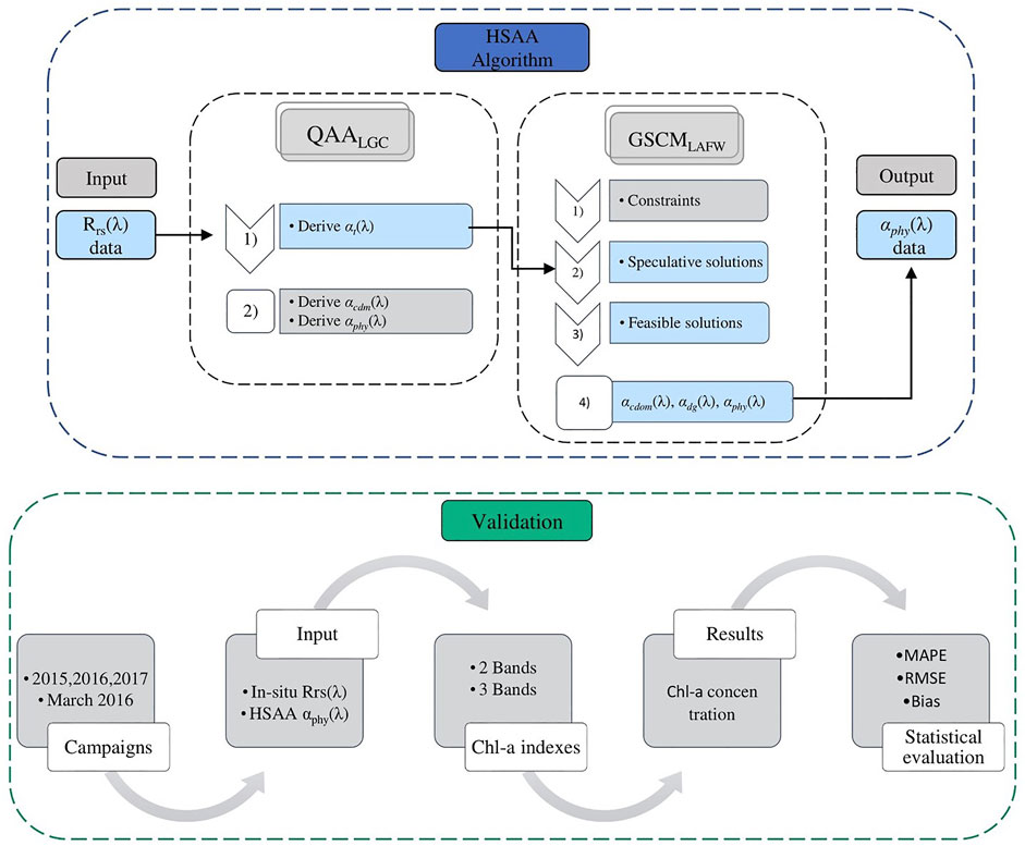
FIGURE 1. Flowchart of the hybrid semi-analytical approach developed in this study (light blue). The Ch-a retrieval and validation steps are presented in green.

2.1 Study Area

The study area comprises five Amazon floodplain lakes located at the Lower Amazon River reach (01º50′S and 55º00′W), around 900 km from the Amazon River mouth, near the cities of Santarem, Óbidos, and Monte Alegre (Figure 2). According to Barbosa et al. (2010), the hydrological regime at that reach can be divided into four stages related to the Amazon River level: 1) the rising waters stage, between January and March, characterized by the Amazon River waters entering the floodplain; 2) the high-water stage, between April and July, when the river and floodplain water level reach a balance; 3) the receding stage, between August and October, characterized by water leaving the lakes toward the Amazon River; and 4) the low stage, from November to December, when the temporary lakes dry and perennial lakes become shallow and turbid. During the rising water, sediment, nutrient, and organic matter rich waters from the Amazon River reach the lakes as channelized fluxes and overbank flows, leading to a complex and lively constituents’ composition, with suspended sediment composition ranging from 36 to 360 mg.L⁻¹ and chlorophyll from 0.20 to 26 μg.L⁻¹ (Barbosa et al., 2010). During high water, the water level balance between the river and lakes reduces the water flux velocity which favors the sedimentation process, and increases light availability in the water column, thus increasing the primary productivity (McClain and Naiman, 2008; Almeida et al., 2015) up to the end of the receding stage. Along these two water-level stages, the chlorophyll-a concentrations span from 1.20 to 350 μg.L⁻¹, and sediment from 5.5 to 200 mg.L⁻¹ (Barbosa et al., 2010). The authors add that at the low water stage, the lakes’ depth reduces to around 1 m, enabling sediment resuspension due to wind stirring favoring suspended sediment concentration of up to 1,000 mg.L⁻¹. Among the selected lakes, Lago Grande Curuai (LGC) stands out, with an open water surface of up to 3,500 km² in the high-water stage decreasing to about 600 km² in the dry season (Bonnet et al., 2008).

FIGURE 2

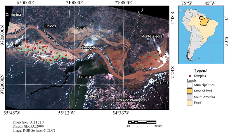
FIGURE 2. Study area with Amazon floodplain lakes: Lago Grande Curuai (LGC), Monte Alegre, Paru, Pacoval, and Aramanaí. Sampling locations are represented as red dots. Background image: true-color composite of Sentinel-3 OLCI image acquired on 16 July 2016.

2.2 In Situ Data

2.2.1 Limnological Data

The dataset (limnological and radiometric) was collected during four field campaigns distributed along the hydrological years spanning from 2015 to 2017 as follows: June/2015 (high water), March/2016 (rising waters), July/2016 (high water), and August/2017 (receding phase). Water samples were collected at the subsurface (∼30 cm) and distributed along 86 sample stations to understand the water constituent’s variability. Water samples were stored in light-free bottles and filtered within nearly 30 min after sample collection. A 250-ml volume of each water sample was filtered through a 47-mm Whatman GF/F (0.7 µm) filter for Chl-a concentration determination (Nush, 1980). A similar volume was filtered through a 47-mm Whatman GF/C (1.2 µm) filter for the determination of the total suspended solid (TSS) concentration and its fractions (inorganic, and organic—TSI and TSO, respectively) (Wetzel and Likens, 2000). The filters were stored frozen (below −20°C) in dark containers until laboratory analysis. For this dataset, the Chl-a ranges from 0.35 to 85 μg.L⁻¹ and suspended sediment from 5.25 to 131.50 mg.L⁻¹. Since field campaigns were not performed during the low water-level stage, sediment load was not as high as reported in the study by Barbosa et al. (2010).

2.2.2 Radiometric Data

Three inter-calibrated spectroradiometers (RAMSES-TRIOS) were used to measure above water total radiance L_t(λ), sky radiance L_sky(λ), and surface incident irradiance E_s(λ). The sensors were positioned nearly 5 m above the water surface to avoid shadow effects and platform reflections. Acquisition geometry was adopted from the study by Mobley (1999). L_t(λ) measurements (W m⁻² sr⁻¹ nm⁻¹) were taken with a 45° zenith angle and nearly 135° azimuth angle from the Sun position to minimize boat-shading and sun-glinting effects (Mobley, 2015). For L_sky(λ) measurements (W m⁻² sr⁻¹ nm⁻¹), the sensor was pointed upward (sky) in the same plane but with a rotation of 45° off-nadir. A cosine sensor pointing upward was also used to measure E_s(λ) (W m⁻² nm⁻¹). Around 150 spectra were acquired within 30 min (∼1 spectrum every 10s) while measuring IOPs in the water column. All data were collected between 10:00 and 14:00 each day. The remote sensing reflectance R_rs(λ) was estimated following the study by Mobley (1999, 2015) as in Eq. (1):

$R_{rs}\left(\text{λ}\right)=\frac{L_t\left(\text{λ}\right)-\rho L_{sky}\left(\text{λ}\right)}{E_s\left(\lambda \right)}\text{, }(1)$

where ρ is a surface reflectance factor calculated with in situ auxiliary data, being wind, time of acquisition, sensor field of view (FOV), latitude, and longitude. As the radiometers acquire data in the range of 320–950 nm and with a spectral resolution of approximately 3.3 nm, E_s(λ), L_t(λ), and the L_sky(λ) measurements were interpolated to 1 nm. These spectra were visually inspected for outlier removal, and then, one spectrum was selected for each sampling station based on its nearness to the dataset median value in the entire spectrum (400–900 nm) (Maciel et al., 2019). As this study focused on OLCI sensor, the R_rs(λ) in situ data was convoluted to its spectral bands based on their spectral response function (ESA, 2015) (Eq. (2)):

$R_{rs}{\left({\text{λ}}_{\text{k}}\right)}_{sim}=\frac{{{\displaystyle \int }}_{{\lambda }_i}^{{\lambda }_j}S\left(\lambda \right)R_{rs}\left(\text{λ}\right)d\text{λ}}{{{\displaystyle \int }}_{{\lambda }_i}^{{\lambda }_j}S\left(\lambda \right)d\text{λ}},(2)$

where $R_{rs}{\left({\text{λ}}_{\text{k}}\right)}_{sim}$ is the OLCI simulated remote sensing reflectance for ${\lambda }_k$ band, λ_i and λ_j are the lower and upper limits, respectively, of each band (λ_k), and S(λ) is the response function for the OLCI bands.

In situ attenuation and absorption measurements were performed with a 10-cm path length attenuation–absorption meter (AC-S) in the spectral range of 400–750 nm and a wavelength resolution of approximately 3.5 nm. Conductivity–temperature–depth (CTD) measurements were acquired using SBE-37SI (Sea-Bird Electronics). The profile was measured at each station as follows: 1) the CTD and AC-S were simultaneously lowered to 75% of the lake depth; 2) they were kept at this depth for around 8 minutes to warm up and to remove air bubbles, as recommended by the manufacturer; and 3) the instruments were slowly raised up to the surface, following the procedures described in the study by Sander de Carvalho et al. (2015). The air-calibration method, as described in the manufacturer’s manual, was run before and after the field campaigns to account for possible instrument drifting. AC-S measurements were conducted for three field campaigns (Jun/2015, July/2016, and August/2017) (n = 58). The Kirk method (Kirk, 1992) was adopted for the scattering correction in the absorption tube according to Sander de Carvalho et al. (2015).

2.2.3 Laboratory Analysis

Water samples for the spectral determination of α_CDOM(λ) (m⁻¹) were filtered through a Whatman nylon filter membrane with 0.22 µm pore size and 47 mm diameter. The CDOM filtered samples were kept cold (not frozen) in a dark container until the laboratory analysis. The samples were measured at room temperature using a 10-cm quartz cuvette in a single beam mode of a 2600 UV–VIS spectrophotometer (Shimadzu, Kyoto, Japan), scanning from 280 to 800 nm, with 1 nm increments using Milli-Q water as a blank reference. The CDOM optical density (OD_med) was measured following the study by Tilstone et al. (2002). The α_CDOM(λ) was determined based on OD_med for each sample station. The optical density values were converted to the absorption coefficient according to the method proposed by Bricaud et al. (1981) (Eq. (3)), where L is the cuvette length in meters (for more information about this protocol, see Silva et al. (2021)).

$a_{cdom}\left(\lambda \right)=2.303\times \frac{O{D}_{med}\left(\lambda \right)}{L}(3)$

Water samples for α_phy(λ) and α_det(λ) measurements were filtered through a 47-mm Whatman GF/F (0.7 µm) filter. These filters were kept frozen and in the dark container until the laboratory analysis. The transmittance–reflectance (TR) method (Tassan and Ferrari, 2002) was used for the determination of α_phy(λ) and α_det(λ). First, the total particulate matter optical density was determined. The filters were then depigmented with sodium chloride and measured again to determine the detritus optical density. The total particulate matter absorption α_p(λ) and α_det(λ) were estimated from the corrected optical densities (Tassan and Ferrari, 1995; 2002). Finally, the α_phy(λ) was obtained by subtracting the α_det(λ) from α_p(λ). The measurements were carried out using the 2600 UV–VIS spectrophotometer with an integrating sphere, scanning from 280 to 800 nm, with 1 nm increments.

2.3 IOP Retrieval Using Hybrid Semi-Analytical Algorithms

In this study, two algorithms were used to obtain the IOPs from R_rs. First, we recalibrated the Quasi-Analytical Algorithm (QAA) using in situ data collected in the Lower Amazon River to derive the total absorption α_t(λ) and backscattering b_b(λ) coefficients. Second, we used a re-parametrized and modified version of the generalized stacked-constraints model (GSCM) algorithm to partition the total non-water absorption coefficient, a_nw(λ) (i.e., the light absorption coefficient without pure-water contribution), into phytoplankton, a_phy(λ), non-algal particulate, a_p(λ), and CDOM, a_CDOM(λ) coefficient. The steps are described in the following sections.

2.3.1 Total Absorption Coefficient Retrieval α_t(λ)

To estimate the α_t(λ), the empirical steps of the quasi-analytical algorithm (QAA) were re-parametrized to the Lower Amazon floodplain waters based on $R_{rs}{\left(\text{λ}\right)}_{sim}$ and α_t(λ) obtained from AC-S (hereafter called QAA_LAFW). The procedure to obtain α_t(λ) is briefly described in the following text:

First, $R_{rs}{\left(\text{λ}\right)}_{sim}$ was converted to subsurface remote sensing reflectance (r_rs(λ)) using Eq. (4), where T and $\gamma Q$ are considered wavelength-independent and can be approximated to $T \sim 0.52$ and $\gamma Q \sim 1.7$ (Lee et al., 2002). Then the relationship between r_rs(λ) and IOPs was computed by Eqs ((5)–(7), with values of g₀ and g₁ of 0.089 and 0.1245, respectively (Lee, 2014).

$r_{rs}\left(\lambda \right)=\frac{R_{rs}{\left(\text{λ}\right)}_{sim}}{T+ \gamma Q{R}_{rs}{\left(\lambda \right)}_{sim}},(4)$

$r_{rs}\left(\lambda \right)=g_0\times u\left(\lambda \right)+g_1\times {\left[u\left(\lambda \right)\right]}^2,(5)$

$u\left(\lambda \right)=\frac{b_b}{a+b_b},(6)$

$u\left(\lambda \right)= \frac{-g_0+\sqrt{[g_0^2+4\times g_1\times r_{rs}\left(\lambda \right)]}}{2\times g_1}.(7)$

The next step was to estimate the α_t(λ₀), where λ₀ is the reference wavelength. In theory, the absorption in the reference wavelength should be dominated by pure water absorption (Lee et al., 2002). In this study, we re-parametrized α_t(λ₀) based on the OLCI band at 754 nm to reduce TSS and CDOM influences on the absorption. Equations (8) and (9) were used for α_t(754) calculation, where ${\alpha }_w\left(754\right)$ is the pure water absorption coefficient at 754 nm, obtained from the study by Pope and Fry (1997). The error (MAPE) of the α_t(754) estimate was 10.51% in relation to the data obtained by the AC-S.

${\alpha }_t\left(754\right)={\alpha }_w\left(754\right)+{10}^{-1.1459-1.3658\chi -0.46927{\chi }^2},(8)$

$\chi =\log \left(\frac{\left(r_{rs}\left(400\right)+r_{rs}\left(413\right)\right)}{r_{rs}\left({\lambda }_0\right)+5\frac{r_{rs}\left(674\right)}{r_{rs}\left(490\right)}{r}_{rs}\left(674\right)}\right).(9)$

Knowing α_t(754), b_bp(754) was analytically derived using Eq. (10), where b_bw($754)$ is the pure water backscattering coefficient obtained from the study by Zhang and Hu (2009). The extrapolation of b_bp($754)$ (Eq. (11)) for all wavelengths requires the power slope of b_bp, which is obtained using an empirical equation (Eq. (12)). Generally, the band ratio used in the QAA is 443/555. In the study, this ratio was defined as 665/754 through the recalibration of the original QAA. The b_bp power slope was not validated because of the lack of in situ data. However, the final validation of α_t(λ) vicariously validates the model performance. Therefore, after knowing b_bp(λ), α_t(λ) was calculated by Eq. (13).

$b_{bp}\left(754\right)=\frac{u\left({\lambda }_0\right)\times a_t\left(754\right)}{1-u\left(754\right)}-b_{bw}\left(754\right),(10)$

$b_{bp}\left(\lambda \right)= b_{bp}\left(754\right)\times {(\text{λ}/\left(754\right))}^{\eta }\text{ ,}(11)$

$\eta =2\left(1-1.2\exp \left(-0.9\frac{r_{rs}\left(665\right)}{r_{rs}\left(754\right)}\right)\right),(12)$

$a_{nw}\left(\lambda \right)=\left(1-u\left(\lambda \right)\right)\times (b_{bw}\left(\lambda \right)+b_{bp}\left(\lambda \right))/u\left(\lambda \right).(13)$

The α_nw(λ) retrievals derived by QAA_LAFW were validated with in situ AC-S α_nw(λ) measurements collected at a sub-surface level (30–70 cm).

2.3.2 Generalized Stacked-Constraints Model (GSCM) for α_phy(λ) Retrieval

The GSCM developed by Zheng et al. (2015) is based on two previous stacked-constraints models (SCM), one of which partitions α_nw(λ) into α_phy(λ) and α_CDM(λ) (Zheng and Stramski, 2013a) and the other which separates the total particulate absorption (α_p(λ)) into α_phy(λ) and α_det(λ) fractions (Zheng and Stramski, 2013b). SCM is a type of model that relies on a set of properly defined inequality constraints for each of the components to realistically determine possible solutions for a given range of optical water type, and GSCM is an extension of SCM for partitioning α_nw(λ) into three components of α_phy(λ), α_det(λ), and α_CDM(λ). GSCM represents an improvement over other semi-analytical approaches as it parameterizes α_det(λ) and α_CDM(λ) slopes in terms of several distinct spectral shapes rather than assuming a common exponential spectral shape for them (Lee et al., 2016a). Moreover, the GSCM accounts for α_det(λ) at the NIR spectral region, which could not be neglected in optically complex waters, improving the model performance at this spectral region. In this study, GSCM was re-parametrized and applied to derive phytoplankton, CDOM, and non-algal particulate absorption contributions to α_nw(λ). To re-parametrize GSCM for the Lower Amazon floodplain turbid waters (hereafter called GSCM_LAFW), we used 83 α_phy(λ), α_det(λ), and α_CDOM(λ) spectra. Moreover, an additional constraint rule was added to account for the high CDOM absorption in Amazon floodplain lakes. The approach described in the study by Zheng et al. (2015) was broken down into three main tasks briefly explained in the following text.

The first task builds α_det(λ), α_CDOM(λ), and α_CDM(λ) spectral libraries to adequately characterize non-algal particles (NAP) and CDOM spectra of the study area. To define a relatively small but representative number of absorption shapes, we normalized each α_det(λ) and α_CDOM(λ) spectra by the integral of their spectral values between 400 and 750 nm, and later, they were grouped according to their spectral shape similarities. The clustering process was carried out using K-means (MacQueen, 1967), with the optimum number of clusters determined by both GAP statistics (Tibshirani et al., 2002) and the Silhouette analysis (Rousseeuw, 1987). The GAP statistic provides a standardized way to define the optimal number of clusters based on the percentage of data variance accounted for each cluster (Tibshirani et al., 2002). The Silhouette measures if a sample is more related to samples within its cluster or to those in other clusters. In practice, a sample silhouette lower than 0 means that it is more related to samples of other clusters and likely to be misclassified, while silhouettes closer to one mean that the sample is likely to be in the right cluster (Rousseeuw, 1987). In this study, we considered the 0.5 value as the optimal number for defining the clusters. The K-means module from the Python scikit-learn (Varoquaux et al., 2015) package was used to compute the clusters. Based on the clustering process, five α_CDOM(λ), and seven α_det(λ) clusters were obtained. Figure 3A,C show the α_CDOM(λ) and α_det(λ) spectral shapes, respectively, and Figure 3C,D show the results of the Silhouette analysis.

FIGURE 3

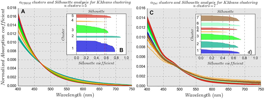
FIGURE 3. (A) α_CDOM(λ) spectral shapes of each cluster; (B) silhouette analysis of α_CDOM(λ) clustering; (C) α_det(λ) spectral shapes of each cluster; (D) silhouette analysis of α_det(λ) clustering. Red dashed lines at (b) and (d) represent the mean value for the silhouette coefficient. The spectral shape colors are the same as the ones in the silhouette cluster colors.

A spectrum representative of each cluster was computed by averaging all spectra within the cluster, resulting in five and seven basic representative spectra shapes for α_CDOM(λ) $\left({\tilde{a}}_{CDOM}\left(\text{λ}\right)\right)$ and for α_det(λ) $\left({\tilde{a}}_{det}\left(\lambda \right)\right)$, respectively. To generate the $\tilde{a}$_CDM(λ) spectral library, we considered it as the sum of $\tilde{a}$_det(λ) and ${\tilde{a}}_{CDOM}\left(\lambda \right)$. The proportions of ${\tilde{a}}_{det}\left(\lambda \right)$ and ${\tilde{a}}_{CDOM}\left(\lambda \right)$ within ${\tilde{a}}_{CDM}\left(\lambda \right)$ composition were represented, as proposed by Zheng et al. (2015), using an array of discrete weighting factors (w_f) ranging from 10 to 90% with 10% increments, which resulted in nine possibilities. It is assumed that both NAP and CDOM are always present and complementary in the water. Therefore, the sum of the weighting factors is always 100%. The combination of ${\tilde{a}}_{det}\left(\lambda \right)$ (7) and ${\tilde{a}}_{CDOM}\left(\lambda \right)$ (5) basic representative spectra shapes with the w_f (9) leads to 315 (7 × 5 × 9) normalized spectral shapes of ${\tilde{a}}_{CDM}\left(\lambda \right)$, which represent all combinations of ${\tilde{a}}_{CDM}\left(\lambda \right)$ basic spectral shapes for our GSCM_LAFW. The set of ${\tilde{a}}_{CDM}\left(\lambda \right)$ is estimated as a linear combination of ${\tilde{a}}_{det}\left(\lambda \right)$ (7) and ${\tilde{a}}_{CDOM}\left(\lambda \right)$ (5) according to Eq. (14):

${\tilde{a}}_{CDM}{\left(\lambda \right)}_k=w_f {\tilde{a}}_{det}{\left(\lambda \right)}_p+(1-w_f){\tilde{a}}_{CDOM}{\left(\lambda \right)}_q ,(14)$

where ${\tilde{a}}_{CDOM}{\left(\lambda \right)}_k$ is the kth spectrum of ${\tilde{a}}_{CDM}\left(\lambda \right)$, k = 1,2, ….315; ${\tilde{a}}_{det}{\left(\lambda \right)}_p$ is the p-th basic spectrum of ${\tilde{a}}_{det}\left(\lambda \right)$, p = 1,2, … 7; and ${\tilde{a}}_{CDOM}{\left(\lambda \right)}_q$ is the q-th basic spectrum of ${\tilde{a}}_{CDOM}\left(\lambda \right)$, q = 1,2, … 5. The 315 spectra of ${\tilde{a}}_{CDM}\left(\lambda \right)$, seven of ${\tilde{a}}_{det}\left(\lambda \right),$ and five of ${\tilde{a}}_{CDOM}\left(\lambda \right)$ constitute a library of spectral shapes for total non-phytoplankton absorption, non-algal particulate absorption, and CDOM absorption, respectively.

The second task was to determine the speculative solutions for α_phy(λ), α_det(λ), and α_CDOM(λ) for each sampling station, based on the ${\tilde{a}}_{CDM}\left(\lambda \right)$ spectral library, on the inequality constraints, and on the α_nw(λ) in 4 wavelengths. The inequality constraints are the rules which ensure that the speculative solutions follow the realistic patterns found in the measured water spectra. Constraints 1 (CS1) and 2 (CS2) are used as speculative solutions for shape simulation of α_phy(λ), α_det(λ), and α_CDOM(λ). For GSCM_LAFW, CS1 (α_phy(412)/α_phy(443)) ranged from 0.85 to 1.5 (32 bins) and CS2 (α_phy(490)/α_phy(443)) from 0.45 to 0.75 (30 bins). Therefore, all the possible speculative solutions are described by a matrix of 32 $\times$ 30 $\times$ 315 (for further information, see Equations (4) to 14) in the study by Zheng et al. (2015)).

The GSCM last task was to determine feasible solutions by filtering the speculative solutions using the inequality constraints 3, 4, and 5 (CS3, CS4, and CS5, respectively). In this study, CS3 (α_phy(469)/α_phy(412)) ranged from 0.55 to 0.83, CS4 (α_phy(555)/α_phy(490)) from 0.35 to 0.67, and CS5 (α_det(750)/α_det(443)) from 0.045 to 0.125. In addition to the standard GSCM, we added an additional constraint (CS6). This constraint is composed of the ratio between αCDOM(750) and αCDOM(443). This modification provides more feasible solutions for αCDOM, considering that αCDOM(443) should always be higher than αCDOM(750). We observe that the ratio between αCDOM(750) and αCDOM(443) is smaller than 1.1% for all our in situ data, which depict highly slopped spectra. Without CS6, the simulations would flatten CDOM absorption spectra not observed in the in situ measurements, causing spectrum underestimation, thus decreasing the model performance. CS6 calibrated to our dataset ranged from 0 to 0.011.

To obtain α_phy(λ) spectra for each sampling station, the feasible solutions of α_det(λ) and α_CDOM(λ) were subtracted from α_nw(λ) values. Then all the feasible solutions that remained after filtration with CS4, CS5, and CS6 were averaged to determine the optimal IOPs (α_det(λ), α_CDOM(λ), and α_phy(λ)) as proposed by Zheng et al. (2015) and Zheng and Digiacomo (2017).

2.4 Chl-a Retrieval

Phytoplankton’s first absorption peak at 443 nm is commonly used for ocean color (e.g., OC2, OC3, and OC4) algorithms to estimate the Chl-a concentration based on blue and green band ratios (Carder et al., 1999; Matthews, 2011; Odermatt et al., 2012). However, in highly turbid waters, high CDOM and particle absorption coefficients at blue and green regions make them unsuitable for Chl-a estimation. As an alternative, algorithms based on red-NIR bands have been used once the influence of the remaining OACs is lower at these wavelengths (Matthews, 2011; Mishra and Mishra, 2012; Odermatt et al., 2012). Therefore, two empirical R_rs(λ) algorithms were tested: 1) two-band (2B) and 2) three-band (3B) algorithms, both from the study by Gitelson et al. (2008). These indexes were tested in their original implementation based on R_rs(λ) (2B-Rrs and 3B-Rrs) (Equations (16) and (18) and based on the HSAA-derived ${\alpha }_{phy}$ (2B-HSAA and 3B-HSAA) (Equations (17) and (19). To apply 2B and 3B HSAA algorithms, they were decomposed in terms of α_phy(λ) and α_w(λ) as proposed by Le et al. (2013) and used by Watanabe et al. (2016). The algorithms were calibrated by the least square method for linear and quadratic fits using a prediction interval with a 0.95 confidence level.

$2B-R_{rs}x=R_{rs}\left(709\right) / R_{rs}\left(665\right)(15)$

$2B-HSAAx=[{\alpha }_{phy}\left(665\right)+{\alpha }_w\left(665\right)] / {\alpha }_w\left(709\right)(16)$

$3B-R_{rs}x=\left[\frac{1}{R_{rs}\left(665\right)} +\frac{1}{R_{rs}\left(709\right)} \right]\ast R_{rs}\left(754\right)(17)$

$3B-HSAAx=\frac{[{\alpha }_{phy}\left(665\right)+{\alpha }_w\left(665\right)- {\alpha }_{phy}\left(709\right)- {\alpha }_w\left(709\right)]}{{\alpha }_w\left(754\right)}.(18)$

2.5 Validation Metrics

To validate the Chl-a algorithms, a Monte Carlo simulation (MC) was used. It consists of randomly selecting samples to calibrate and validate the proposed algorithm. This process was repeated several times (20000) in which 70% of the dataset is used for calibration (n = 58) and 30% for validation (n = 25). The validation metrics were Pearson (R), the mean absolute percentage error (MAPE), root mean square error (RMSE), and BIAS (Equations ((20)–(22), respectively).

$MAPE=\frac{{{\displaystyle \sum }}_{i=1}^n\left|\frac{x_i^{est}-x_i^{obs}}{x_i^{obs}}\right|}{n}\text{*}100,(19)$

$RMSE=\sqrt{\frac{1}{n}{\displaystyle \sum }_{i=1}^n{\left(x_i^{est}-x_i^{obs}\right)}^2},(20)$

$Bias=\frac{1}{n}{\displaystyle \sum }_{i=1}^n\left(x_i^{est}-x_i^{obs}\right).(21)$

where “est” are the estimated values, “obs” are the measured values, n is the number of samples, and σ is the standard deviation.

2.6 Algorithm Validation for Sentinel-3/OLCI Images

For the algorithm application and its validation, three Sentinel-3 OLCI images were selected (16 July 2016 (n = 9), 06 August 2017 (n = 14), and 28 August 2019 (n = 14)). Note that the 2019 campaign was used only for validation of the algorithm due to the unavailability of in situ IOPs. The enhanced full resolution top-of-atmosphere radiance product was downloaded from the Copernicus database, and then, the atmospheric correction was applied using the second simulation of satellite signal in the solar spectrum vector version (6SV) algorithm (Vermote et al., 2006). 6SV is a physical-based atmospheric correction method that allows simulating atmospheric effects based on the radiative transfer theory. As input data, 6SV requires atmospheric parameters such as ozone, aerosol optical depth, and water vapor, and other auxiliary information such as sun-view angles, spectral response function of the sensor, date, and time of image acquisition. The atmospheric parameters were obtained from MODIS atmospheric products (MOD04 and MOD08) using the Google Earth Engine platform (Martins et al., 2017). For the application of the 6SV, the AtmosPy package was used to automate the correction procedure (Carlos et al., 2019). The 6SV has been successfully used to correct atmospheric effects of Sentinel-2 and Landsat-8 data across different Brazilian inland waters (Cairo et al., 2020; Curtarelli et al., 2020; Maciel et al., 2020). For algorithm validation, the pixel values corresponding to the in situ station were extracted for each corresponding OLCI image. Note that a time gap interval of ±5 days was selected in this study for the matchups. The time gap between in situ measurements and the satellite overpass is a well-known problem in other inland water studies that need to be adjusted for a sufficient sample number (Kloiber et al., 2002; Olmanson et al., 2008; Sriwongsitanon et al., 2011), and the reasonable interval is typically dependent on lake and hydrological conditions of the region. In this study, the field data collection was performed in a wet season where the river-floodplain water exchange is a slow and gradual process, and water level remains stable for days. Moreover, all measurements were collected under clear-sky conditions and low wind speed (<5 m/s) that minimize water circulation and sediment resuspension. For these reasons alongside with the fact that a time gap of ±5 days presented a negligible impact on the data comparison in studies presented by Barbosa et al. (2009) and Maciel et al. (2019), the time gap was considered appropriate.

3 Results

3.1 Water Quality and Radiometric Data Variability

The quantities of limnological parameters measured in situ, as well as the Secchi and water bodies depths, can be observed in Table 1. Chl-a in situ concentration in this study spanned from 0.35 μg.L⁻¹ to 85.05 μg.L⁻¹, with an average of 14.51 μg.L⁻¹ and TSS concentrations ranged from 5.25 to 131.5 mg.L⁻¹, with a higher TSI contribution (mean values of TSI/TSS ratio of 61.75%). The Secchi disk depth varied from 0.12 to 1.15 m and lake depth from 1.8 to 7.7 m along with the field campaigns, in response to the Amazon River hydrological phases. The TSI/TSS ratio throughout all campaigns ranged from 28 to 86%. However, the average ratios of the campaigns (55% in 2015, 70 and 58% in 2016, and 66% in 2017) indicate a major influence of inorganic matter, since the lowest average was 55%.

TABLE 1

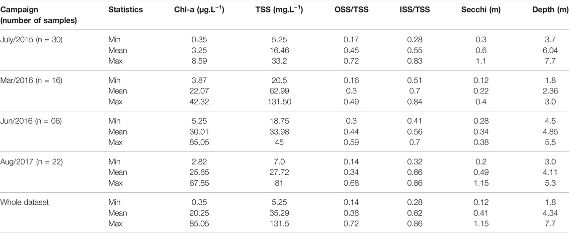
TABLE 1. Minimum (min), mean, and maximum (max) values for Chl-a, TSS, TSO/TSS ratio, TSI/TSS ratio, Secchi disk depth, and water depth for each campaign.

The observed OACs variability for each campaign was also present in the OLCI simulated in situ R_rs(λ) (Figure 4). The lower reflectance at wavelengths below 500 nm in all campaigns was mainly explained by high CDOM and detritus absorption. None of the phytoplanktonic diagnostic pigment features occurred in the blue spectral region. Between 550 and 650 nm, there were fluctuations in the R_rs(λ) magnitude but without any significant change in the spectra shape. Spectra magnitude variation can be associated with particulate concentration fluctuations, which modifies the backscattering coefficient, due to an increase in TSS concentration. The low Chl-a concentration in 2015 (Figure 4A) prevented the detection of pigment absorption bands. In Jun/2016 (Figure 4C) and Aug/2017 (Figure 4D) campaigns, for some in situ measured spectra, the Chl-a absorption peak is well defined around 675 nm.

FIGURE 4

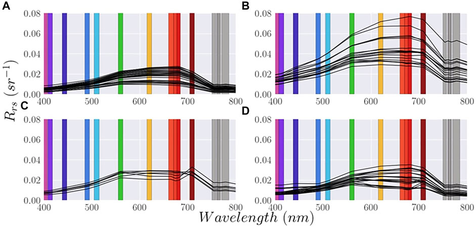
FIGURE 4. R_rs(λ) simulated for OLCI bands in (A) July/2015 (n = 30), (B) March/2016 (n = 16), (C) Jun/2016 (n = 06), and (D) Aug/2017 (n = 22). The colors bars are representative to OLCI bands in the true visible colors of the electromagnetic spectrum and NIR.

Figure 5 presents the relative contribution of IOPs absorption (phytoplankton, CDOM, and detritus) at 400, 443, 560, and 665 nm, corresponding to the Oa01, Oa03, Oa06, and Oa08 OLCI bands. At 400 nm, α_det(400) and α_CDOM(400) contributions to the total absorption (a_nw(400)) were 48.8 and 28.2% (median values), respectively, and confirm the dominance of α_det. At 443 nm, α_det(443) maintained its dominance with a median of 46.6% of total absorption, whereas α_CDOM(443) and α_phy(443) had similar but much lower values of 25.8 and 27.6%, respectively. At 560 nm, α_CDOM(560) was heavily reduced to 16.8%, whereas α_det(560) kept similar to 443 nm (46.2%), and the α_phy(560) contribution increased to 37.0%. Finally, at 665 nm, the influence of α_phy(λ) became dominant, with a median of 56.2%, despite its wide variability, ranging from 40 to 85% (Figure 5D), while α_CDOM(λ) was reduced to 5.7% of total absorption.

FIGURE 5

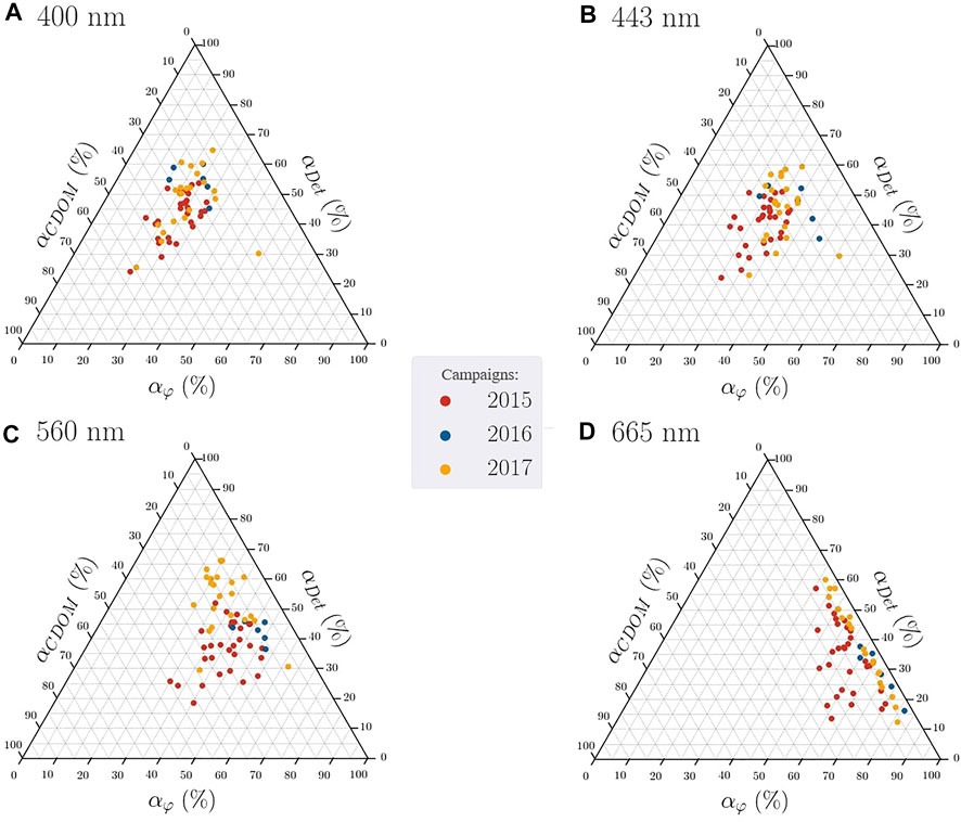
FIGURE 5. Phytoplankton, CDOM, and detritus absorptions at OLCI bands (A) Oa01, (B) Oa03, (C) Oa06, and (D) Oa08. Note that campaigns 2015, 2016, and 2017 refer to Jul/2015, July/2016, and Aug/2017, respectively. The α_nw was calculated based on the sum of laboratory-measured IOPs (α_nw = α_CDOM + α_phy + α_det).

3.2 IOP Retrieval

3.2.1 α_t(λ) Retrieval

The first step of the HSAA is to accurately retrieve the total absorption coefficient (α_t), which will afterward be used in the GSCM algorithm. The results demonstrated the feasibility of the recalibrated QAA proposed in this study, as the MAPE values were lower than 31.28% for α_t in the range between 400 and 750 nm (Table 2). For the blue bands (400, 413, 443, and 490 nm), the MAPE values were lower than 25.15%; however, Pearson R varied between 0.5 (at 400 nm) and 0.8 (at 443 and 490 nm). For the green bands (510 and 560 nm), the MAPE values were 15.74% (510 nm) and 26.19% (560 nm) with a Pearson R of 0.77 and 0.72, respectively. For red bands (620, 665, 674, and 681 nm), the MAPE values were relatively stable at approximately 30%, and Pearson R values were around 0.6. Finally, for the 709 nm red-edge band, MAPE was 28.94%, with a Pearson R of 0.43. Therefore, the results show that these errors are relatively low, mainly in the key bands to chlorophyll-a retrieval (e.g., the red and red-edge bands). Moreover, the algorithm was able to accurately identify the α_t for blue bands, which is a relevant result considering the highly absorbing environment.

TABLE 2

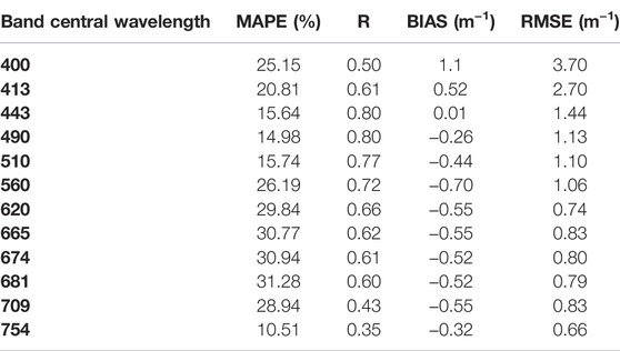
TABLE 2. Statistical results of α_t(λ) retrieval for OLCI bands.

3.2.2 α_Phy Retrieval From GSCM

In the second step, α_t was partitioned into its fractions α_det(λ), α_CDOM(λ), and α_phy(λ). Due to the optical complexity of the Amazon floodplain waters, the accuracy of α_phy(λ) retrieval using the QAA framework (see Supplementary Files S1) was unsatisfactory (MAPE >38%), demanding other methods for better determination. The GSCM algorithm filled the accuracy gap observed in the SAA algorithm regarding α_phy(λ) retrieval (Figure 6). The GSCM results provided MAPE values lower than 24% for α_phy(λ) estimates in the visible bands. For example, Pearson R for α_phy(443) was 0.88, with MAPE values of 23.49%. For Chl-a absorption bands (665 and 674 nm), MAPE was lower than 20%, with Pearson R higher than 0.95. The new proposed algorithm outperformed the QAA; its best results was a MAPE of 38.73%, and a Pearson R of 0.75 for 674 nm. These results indicate that our re-parametrized GSCM_LAFW provided accurate results for the Amazon floodplain optically complex waters.

FIGURE 6

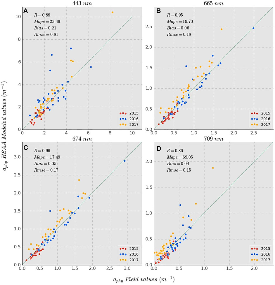
FIGURE 6. α_phy(λ) retrieval for HSAA at (A) 443 nm, (B) 665 nm, (C) 674 nm, and (D) 709 nm.

3.3 Chl-a Concentration Retrieval From IOPs

Chl-a concentration retrieval was evaluated using 2B and 3B algorithms (Le et al., 2013) based on in situ measured R_rs(λ)_sim, and on α_phy(λ) derived from the HSAA (α_phy(λ)_HSAA) (Table 3). The results from the validation based on the Monte Carlo simulation showed that the 3B-α_phy(λ)_HSAA polynomial (quadratic) algorithm (3B-HSAA) outperformed the remaining algorithms when predicting Chl-a concentration. The mode of MAPE for that algorithm was 36.94%, with R of 0.94, and BIAS of 0.05, indicating good agreement between in situ measured and α_phy(λ)_HSAA-derived Chl-a concentration. Comparatively, the HSAA-based algorithm outperformed R_rs-based algorithms. Despite the high Pearson R values (0.90–0.94), MAPE values are higher than 73% for these R_rs-based algorithms. To further evaluate the algorithms’ performance, Figure 7 presents the scatterplots of in situ measured versus Chl-a concentration obtained from R_rs(λ) and α_phy(λ)_HSAA algorithms. The scatterplot between predicted and measured Chl-a concentration also demonstrated the accuracy of the 3B-HSAA algorithm to estimate Chl-a in optically complex waters, with results closer to the 1:1 line.

TABLE 3

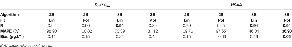
TABLE 3. Statistical results obtained from Monte Carlo simulation for chlorophyll-a algorithms using 2-band (2B) and 3-band (3B) algorithms with linear (Lin) and quadratic polynomial (Pol) fitting.

FIGURE 7

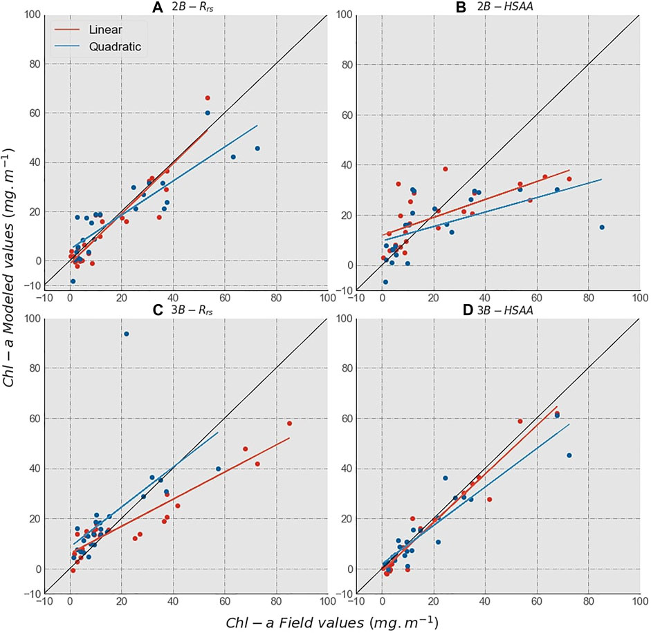
FIGURE 7. Scatterplot between field-measured Chl-a and estimated Chl-a with (first row) 2B algorithm using (A) R_rs(λ)_sim and (B) HSAA; and (second row) 3B algorithm using (C) R_rs(λ)_sim and (D) and HSAA. Red data refer to the model developed using linear fit, while blue data refer to the algorithm developed using quadratic fit. Note that the data in each plot correspond to the validation dataset that is closer to the mode of MAPE values and may not be the same in all plots.

3.4 Application to Sentinel-3/OLCI Data

To demonstrate the applicability of HSAA for estimating Chl-a concentration using OLCI data, we obtained three OLCI images at Lago Grande do Curuai. First, the accuracy of atmospheric correction was assessed by comparing R_rs(λ)_sim with R_rs(λ)_OLCI. The accuracy of the 6SV did not present a reasonable correlation in the blue band, possibly due to the low R_rs caused by the high CDOM and suspended sediment absorption (Table 4). The results were better from green (560 nm) toward the red edge. MAPE values were between 17.32% (665 nm, Pearson R of 0.86) and 72.27% (754 nm, Pearson-R of 0.73), indicating good agreement between satellite and in situ measured R_rs.

TABLE 4

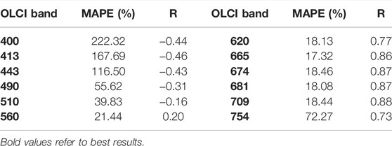
TABLE 4. Validation of atmospheric correction using 6SV algorithm (n = 45).

Once the atmospheric correction was validated, R_rs(λ)_OLCI was used as an input to the HSAA to retrieve α_phy(λ), and this result was used as an input to the 3B polynomial (quadratic) algorithm to obtain Chl-a concentration (Figure 8). The results demonstrated that the errors were 57%, with Pearson-R of 0.86, BIAS of -17.88, and RMSE of 20.21 μg.L⁻¹, indicating the reasonability of using this algorithm applied to OLCI images to estimate Chl-a concentration in optically complex waters. However, uncertainties were also higher than those obtained for field data. This could be attributed to the errors in atmospheric correction (>39% for wavelengths lower than 510 nm), absence of glint correction, and the spatial resolution of the OLCI sensor. The influence of atmospheric correction makes the blue band less reliable than longer wavelengths due to the strong atmospheric scattering causing uncertainties in the Chl-a retrieval derived from the HSAA framework. Therefore, more accurate methods for retrieving the high-quality R_rs products from OLCI images were needed.

FIGURE 8

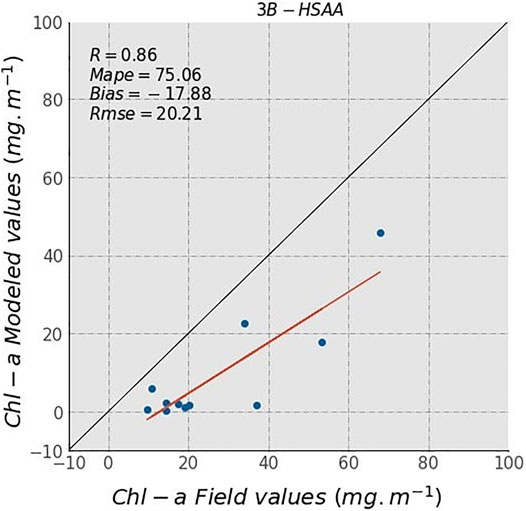
FIGURE 8. Scatterplot between field-measured Chl-a and estimated Chl-a with the HSAA-3B algorithm. Note that the sample size is lower due to negative values (n = 26).

4 Discussion

In this study, we implemented a novel hybrid semi-analytical algorithm (HSAA) that combines a re-parameterization of quasi-analytical algorithm (QAA) (Lee., 2014) with an improved version of generalized Generalized Stacked-Constraint Model (GSCM) (Zheng et al., 2015; Zheng and Digiacomo, 2017) focusing on the Sentinel-3 OLCI data. The new algorithm accurately estimated the phytoplankton absorption coefficient (α_phy(λ)_HSAA) with errors smaller than 24% in the visible bands. The HSAA Chl-a retrievals with two- and three-band algorithms (using spectral α_phy input) were validated with in situ Chl-a measurements and compared to the commonly used R_rs empirical-based algorithms. The results demonstrated that the 3B-HSAA algorithm outperformed the 3B-R_rs-based algorithms for Chl-a concentration retrieval (MAPE of 35%). The proposed algorithm was applied and validated in OLCI images to provide a synoptic view of Chl-a in lower Amazon floodplain lakes.

4.1 In Situ OACs and R_rs(λ) Variability

The medium-to-high suspended sediment concentrations (mean = 35.28 mg.L⁻¹) observed in this study limit the observation of Chl-a absorption features in R_rs spectra (Figure 3). During the 2015 field campaign, the mean Chl-a concentration was 3.25 μg.L⁻¹, with a mean TSS concentration of 16.46 mg.L⁻¹. This pattern can be attributed to the high water level of the Amazon River (Barichivich et al., 2018), which increases the inflow toward the floodplain lakes, bringing sediments and organic matter. Thus, as turbulence increases, the availability of light decreases, leading to a reduction of the phytoplankton growth rate (Barbosa et al., 2010; Rudorff et al., 2018). For June 2016 and August 2017 field campaigns (beginning of receding water phase), high values of Chl-a (mean of 30.01 and 25.65 μg.L⁻¹, respectively) are attributed to nutrients supplied to the lakes during rising and high water stages (Dunne et al., 2010; Silva et al., 2013; Bonnet et al., 2017). Moreover, CDOM and TSS input from the Amazon River into the floodplain decrease in these stages, resulting in higher light availability supporting phytoplankton growth (Martinez et al., 2015; Maciel et al., 2020).

The influence of hydrograph phases over OACs’ concentration and, consequently, on R_rs(λ) spectra was also observed in other studies (Barbosa et al., 2010; Fassoni-Andrade and Paiva, 2019; Maciel et al., 2019). The low intensity in the R_rs(λ) spectrum for 2015 and 2017 campaigns can be attributed to low TSS and TSI concentrations (mean of 16.46 and 27.72 mg.L⁻¹, respectively). For June 2016, a drought in the Amazon Basin led to higher TSS and TSI (mean of 33.98 mg.L⁻¹ of TSS with 56% being TSI), due to lower water levels in floodplain lakes, than those of August 2017 (Barichivich et al., 2018). For March 2016 (rising water stage), high TSS (mean of 62.99 mg.L⁻¹) with 70% being TSI resulted in high magnitude R_rs(λ) spectra. Thus, R_rs(λ) also combined into two different groups due to the high variability in amplitude and proportion of OACs in the March campaign. Furthermore, the mean TSI/TSS ratio presented high values (∼72%), indicating a high concentration of inorganic sediments related to the input of the Amazon River sediments through river channels at rising water (Barbosa et al., 2010; Rudorff et al., 2018).

4.2 HSAA Parametrization and Uncertainties: QAA and GSCM Improvements

The first step of the quasi-analytical algorithm is the selection of λ₀. The main assumption of this step is that total absorption is dominated by pure water (Lee et al., 2002). In this study, we used the 754 nm OLCI band as it improves the results and it was also used by other authors in turbid environments (Yang et al., 2014; Watanabe et al., 2016). The next step in the QAA implementation is to empirically parameterize the residual influence of the OACs in the absorption at λ₀ (α_t(λ₀)). The selected bands need to be related to the environment characteristics regarding OAC proportions, considering the residual influence of particulate matter, CDOM, and phytoplankton (Mishra et al., 2013; Mishra et al., 2014; Watanabe et al., 2016). Due to the small influence of Chl-a on the total absorption in Curuai Lake data (Figure 5), the selected bands aimed to compensate for the remaining influence of the TSS and CDOM, being 400, 413, 674, and 490 nm. This empirical selection presented errors of 11% at 754 nm band (see Table 2). In addition, the backscattering coefficient slope (η factor) has high influence on α_t(λ) estimates (Lee et al., 2002; Yang et al., 2013; Rodrigues, 2017). In the original versions, QAAs propose an empirical ratio using R_rs(λ) that should be re-parametrized based on in situ data (Lee et al., 2009; Lee, 2014). The assessment of several band ratios indicated 665/754 nm as the best to derive η, the same ratio used by Rodrigues (2017). The η values obtained by QAA ranged from 1.28 to 1.98 with an average of 1.79, which corroborate with in situ data observed for Curuai lake by Sander de Carvalho. (2016). Typically, these values range from 0 to 2.2, with higher values associated with backscattering by small particles (Roesler and Boss, 2008). The accuracy of the recalibrated QAA algorithm was evaluated based on the results of α_t(λ). Errors were between 14 and 30% for the visible and NIR bands (at up to 754 nm), indicating a good agreement between predicted and measured α_t(λ). These results agree with a recalibrated QAA based on Sentinel-2/MSI on the Lower Amazon lakes (Maciel et al., 2020), where authors obtained errors between 20 and 35% for the α_t(λ) estimates, with higher errors for the red bands (∼35%), like those obtained in our study.

The adequate estimation of α_t(λ) from QAA is essential to its decomposition into the specific absorption components α_CDM(λ) and α_phy(λ). In this study, the GSCM approach was used. Although the GSCM may not be as fast-forward as other semi-analytical models to derive α_phy(λ) such as QAA, it represents a new and unexplored approach to complex waters. The GSCM also requires computational efforts, and as stated by Zheng et al. (2015), it may not give feasible solutions. However, in this study, our dataset provided enough groups to represent the aquatic environment variability without expanding the processing time. It was also fundamental to calibrate the inequality constraints for both spectra simulation and filtering, as our data range visibly differs from the original GSCM. The addition of a new constraint (CS6) to the GSCM_LAFW was key to make CDOM simulations realistic. When the performance of the α_phy(λ) retrieved from GSCM and QAAs was compared, GSCM_LAFW provided much more precise results, with R higher than 0.88 and MAPE lower than 25% for 443, 665, and 674 nm bands.

Given the results from HSAA, it represents a feasible solution for decomposing the IOPs in turbid complex waters. The framework presented comprises two well-known semi-analytical models which are reliable and accurate in state-of-the-art literature. Moreover, as both models allow calibration, the HSAA can be applied in other aquatic environments.

4.3 IOP Algorithms to Derive Chl-A Concentration

The empirical algorithms derived with in situ measured R_rs(λ) data did not present satisfactory performance (Table 3). These errors may be attributed to the lack of relationship between Chl-a and R_rs(λ) due to the high scattering of the inorganic particle, typical of Amazonian turbid waters, which affects phytoplankton absorption features (Lee et al., 2016a). In this sense, the best result was achieved using the 3-B α_phy(λ)_HSAA with a quadratic fit. The GSCM approach improved the accuracy compared to R_rs(λ), or QAA derived α_phy(λ) for Chl-a retrieval, as reported by Zheng and Digiacomo (2017). The authors observed that GSCM provided more accurate results using GSCM-derived α_phy(λ) (e.g., R = 0.66 and mean percentage difference = 31% for Chl-a estimated by α_phy(670) algorithm using VIIRS sensor). However, it should be noted that Zheng and Digiacomo (2017) applied only α_phy(670) to parameterize a Chl-a algorithm. In our research, we used a 3B algorithm because it provided better results. The increase in accuracy using band ratios or IOPs band combinations algorithms was also demonstrated by other authors (Le et al., 2013; Watanabe et al., 2016; Rotta et al., 2021). For example, Watanabe et al. (2016) observed that band ratios with QAA-derived α_phy(λ) (MAPE = 25.31%) outperformed other empirical algorithms (MAPE = 69.06%) in the estimation of Chl-a concentration (up to 550 µg.L⁻¹) in a Brazilian eutrophic reservoir.

Considering the algorithm applied to the Sentinel-3 OLCI imagery, the results presented reasonable accuracy (MAPE = 57%). The result observed in this study was in alignment with recent works with Chl-a retrieval using OLCI data. For example, Pahlevan et al. (2020) observed errors of 55.6% on Chl-a retrieval using the mixture density network across several lakes in North America. Kravitz et al. (2020) obtained an RMSE of 107% and R² of 0.35 for Chl-a retrieval in four small dams with an empirical algorithm using maximum chlorophyll index (MCI). It indicates that the HSAA proposed in this study agrees with the results obtained in the literature for the OLCI sensor. The comparison between in situ and orbital data is affected by different sources of uncertainty such as inaccurate atmospheric correction, time gap interval, specular reflectance, instrument characteristics, and bidirectional reflectance distribution function (BRDF) effects. Regarding these sources, standard protocols in data collection were adopted to minimize the difference between in situ and orbital data. For example, the data collection was restricted to a short time window (10 a.m.—2 p.m.) and close to the sensor overpass which minimizes the solar zenith differences. Moreover, field sensor zenith and azimuth angles were fixed, as suggested by Mobley (1999), and all measures were corrected by sky radiance (Section 2.2.2). For OLCI data, an atmospheric correction was performed with a well-known 6SV model, also used by MODIS and Landsat surface reflectance products. The BRDF correction is desirable though BRDF coefficients for normalization are not available for the Sentinel-3 OLCI sensor, and this additional analysis is out-of-scope for this study.

Another source of errors is the atmospheric correction, especially in OLCI blue bands. The errors and uncertainties in the blue region are well reported in the literature (Gossn et al., 2019; Vanhellemont and Ruddick, 2021). These errors are associated with uncertainties in the atmospheric scattering, caused by the presence of molecule and aerosol particles in the atmospheric layer. Both the aerosol particles and molecules are responsible for the extinction (absorption and scattering) of the radiation that leaves the water surface toward the sensor. When the aerosol loading is high, the magnitude of the atmospheric scattering surpasses the ground reflectance at the top-of-atmosphere and, consequently, imposes the challenge of atmospheric correction of remote sensing images (Martins V. et al., 2017). In the Amazon region, huge variability and quantities of aerosol particles in the atmosphere are expected due to the frequent occurrence of fires in the dry season (Martins et al., 2018). According to Martins V. S. et al. (2017), the aerosol optical depth at 550 nm, the parameter used to measure the scattering and absorption of the radiation due to aerosol, in some Amazon regions can range from 0.25 to 1.0 during most of the year’s months. These values indicate the atmosphere’s optical complexity, and the difficulty to estimate the water reflectance accurately in this region. Moreover, the contrast between the atmosphere scattering and the water surface is preferentially pronounced at blue wavelengths (Martins V. et al., 2017), due to greater scattering by atmospheric constituents, and high absorption coefficient in the water, attributed to CDOM and suspended materials, making the R_rs at this region small (Sander de Carvalho et al., 2015; Maciel et al., 2020).

Moreover, the 6SV atmospheric correction method used in this study did not perform any correction for glint effects. It was observed that with Sentinel-2, a simple glint correction by subtracting the SWIR band from the VNIR could reduce uncertainties in atmospheric corrections by 80% in Curuai Lake (Maciel et al., 2019). Therefore, these three facts could be interfering in the accuracy of R_rs retrieved from OLCI in blue bands (MAPE >39%). The importance of the blue band in the HSAA realizes on the fact that the parametrization of QAA and GSCM is based on several bands in this region (e.g., Eq. (9)). Therefore, small uncertainties could be impacting the results. Moreover, another uncertainty observed is the negative Chl-a values obtained from the HSAA approach. These negative values are attributed to the fact that α_phy(709) are given values closer to the α_phy(665), and the 3B model parameterized with the in situ data did not present these values. This could be related to the uncertainties observed in atmospheric and glint correction. It could be also inferred that the errors are attributed to the fact that the suspended sediment masks the small signal of Chl-a in the 664 nm band, and the errors in OLCI R_rs obtention are preventing high-quality data of surface reflectance. For further reference, we observed that an important step when developing algorithms based on in situ data to be applied to satellites is the development of algorithms based on bands with a lower uncertainty in atmospheric correction (Jorge et al., 2017). For example, Maciel et al. (2021) developed a random forest algorithm for estimating Secchi disk depth in Brazilian waters based on in situ R_rs. Despite the availability of R_rs data between 400 and 900 nm, only bands between 490 and 740 nm were used due to errors in atmospheric correction. These errors, when propagated to the satellite data, could be an important source of errors (Silva et al., 2021). However, despite the observed uncertainties, this algorithm represents an important development for remote sensing estimates of optically active constituents in the Amazon region. This work is an important contribution to the estimative of Chl-a years in Amazon lakes, as the last study focused on retrieval of Chl-a concentration using satellite data in the Amazon region was dated from 2006 (Novo et al., 2006). Therefore, this study is important and necessary to present an alternative method for Chl-a retrieval in optically complex waters (Fassoni-Andrade et al., 2021). However, it is important to point out that this study has implemented generic empirical models for comparison, but there is extensive literature on the topic and further studies are recommended to compare the recent models using different band ratios or even machine learning approaches.

5 Conclusion

In this study, we proposed a hybrid semi-analytical algorithm (HSAA) to retrieve the inherent optical properties (IOP) of the five Amazon floodplain lakes, and then estimate Chl-a concentration using IOP indexes algorithms. The algorithm is based on re-parameterizations, and improvements of the quasi-analytical algorithm (QAA) combined with the generalized stacked constraints model (GSCM). The use of HSAA presented errors between 15 and 35% for α_t(λ) estimates in Amazon waters. After α_t(λ), α_phy(λ) was implemented. However, α_phy(λ) retrieval using re-parametrized QAA did not achieve reasonable results (MAPE greater than 50% in the visible bands). Thus, an improved GSCM was applied to better estimate α_phy(λ), and consequently, Chl-a concentration retrieval using two- and three-band algorithms. The results obtained with HSAA α_phy(λ) retrieval were more accurate than those with QAA (being the lowest MAPE = 17.49% and R = 0.96). Regarding Chl-a estimates, the 3-B α_phy(λ)_HSAA algorithm achieved the most accurate results (MAPE = 36.93% and R = 0.94). Using the calibrated model, Chl-a concentration was applied to Sentinel-3 OLCI images. The results demonstrated the algorithm’s feasibility in retrieving Chl-a concentration with OLCI data, with errors of 57%. However, challenges are still imposed by an accurate atmospheric correction in shorter wavelengths, which increased the uncertainty of the proposed algorithm when applied to satellite data. Considering the lack of studies on optical water properties in the Amazon regions, the proposed HSAA becomes the first step in developing a Chl-a monitoring system in these turbid environments. Also, considering that the R_rs(λ) is the only input to HSAA, it has great potential for future applications with satellite optical images, especially with OLCI sensor due to its radiometric quality (signal-to-noise ratio), band suitability for OAC retrieval, and high temporal/spatial coverage.

Data Availability Statement

The original contributions presented in the study are included in the article/Supplementary Materials; further inquiries can be directed to the corresponding author.

Author Contributions

FJR, CFB, and DAM conceived the presented idea. FJR and FMC designed the computational framework and carried out the implementation. FJR processed the experimental data, performed the analysis, drafted the manuscript, and designed figures. FJR and DAM wrote the manuscript with input from all authors. VSM, FLL, and LSC were involved in all decision-making processes related to the manuscript. FJR, VSM, DAM, CFB, and EMN. actively participated in the manuscript reviews. All authors discussed the results and contributed to the final manuscript. CFB and EMN supervised the project.

Funding

This research was funded through the 2017‐2018 Belmont Forum and BiodivERsA joint call for research proposals, under the BiodivScen ERA-Net COFUND program, and with the funding organizations, namely, the French National Research Agency (ANR), the São Paulo Research Foundation, and the National Science Foundation (NSF), the Research Council of Norway, the German Federal Ministry of Education and Research (BMBF), and the Foundation BNP Paribas through SABERES Project. The field campaigns were sponsored by the project MAS-BNDES code 1022114003005. This work was supported in part by Fundação de Amparo à Pesquisa do Estado de São Paulo (FAPESP) (2014/23903-9, 2018/12083-1), by MAS-BNDES (1022114003005), by Coordenação de Aperfeiçoamento de Pessoal de Nível Superior, Brasil (CAPES), Finance Code 001; and by the Brazilian National Council for Scientific and Technological Development (CNPq). Finally, the first author would like thank the French embassy in Brazil through CAMPUS FRANCE for the Ph.D Scholarship.

Conflict of Interest

The authors declare that the research was conducted in the absence of any commercial or financial relationships that could be construed as a potential conflict of interest.

Publisher’s Note

All claims expressed in this article are solely those of the authors and do not necessarily represent those of their affiliated organizations, or those of the publisher, the editors, and the reviewers. Any product that may be evaluated in this article, or claim that may be made by its manufacturer, is not guaranteed or endorsed by the publisher.

Acknowledgments

The authors would like to thank Rejane Paulino for her help in review and with insights about atmospheric correction. The authors are also grateful to Daniel Meneghetti for laboratory support and to Laquatec/CCST/INPE for providing access to laboratory facilities.

Supplementary Material

The Supplementary Material for this article can be found online at: https://www.frontiersin.org/articles/10.3389/frsen.2022.834576/full#supplementary-material

References

Almeida, R., Tranvik, L., Huszar, V., Sobek, S., Mendonça, R., Barros, N., et al. (2015). Phosphorus Transport by the Largest Amazon Tributary (Madeira River, Brazil) and its Sensitivity to Precipitation and Damming. Iw 5, 275–282. doi:10.5268/IW-5.3.815

CrossRef Full Text | Google Scholar

Barbosa, C. C. F., de Moraes Novo, E. M. L., Melack, J. M., Gastil-Buhl, M., Filho, W. P., de Moraes Novo, E. M. L., et al. (2010). Geospatial Analysis of Spatiotemporal Patterns of pH, Total Suspended Sediment and Chlorophyll-A on the Amazon Floodplain. Limnology 11, 155–166. doi:10.1007/s10201-009-0305-5

CrossRef Full Text | Google Scholar

Barbosa, C. C. F., Novo, E. M. L. M., and Martinez, J. M. (2009). "Remote Sensing of the Water Properties of the Amazon Floodplain Lakes: The Time Delay Effects between In-Situ and Satellite Data Acquisition on Model Accuracy," in Proceedings, 33rd International Symposium on Remote Sensing of the Environment, Stresa, Italy, May 5-9, 2002, 732, TS-57-5.

Google Scholar

Barichivich, J., Gloor, E., Peylin, P., Brienen, R. J. W., Schöngart, J., Espinoza, J. C., et al. (2018). Recent Intensification of Amazon Flooding Extremes Driven by Strengthened Walker Circulation. Sci. Adv. 4, eaat8785. doi:10.1126/sciadv.aat8785

PubMed Abstract | CrossRef Full Text | Google Scholar

Behrenfeld, M. J., and Falkowski, P. G. (1997). A Consumer's Guide to Phytoplankton Primary Productivity Models. Limnol. Oceanogr. 42, 1479–1491. doi:10.4319/lo.1997.42.7.1479

CrossRef Full Text | Google Scholar

Bonnet, M.-P., Pinel, S., Garnier, J., Bois, J., Resende Boaventura, G., Seyler, P., et al. (2017). Amazonian Floodplain Water Balance Based on Modelling and Analyses of Hydrologic and Electrical Conductivity Data. Hydrol. Process. 31, 1702–1718. doi:10.1002/hyp.11138

CrossRef Full Text | Google Scholar

Bonnet, M. P., Barroux, G., Martinez, J. M., Seyler, F., Moreira-Turcq, P., Cochonneau, G., et al. (2008). Floodplain hydrology in an Amazon floodplain lake (Lago Grande de Curuaí). J. Hydrol. 349, 18–30. doi:10.1016/j.jhydrol.2007.10.055

CrossRef Full Text | Google Scholar

Bricaud, A., Morel, A., and Prieur, L. (1981). Absorption by Dissolved Organic Matter of the Sea (Yellow Substance) in the UV and Visible Domains1. Limnol. Oceanogr. 26, 43–53. doi:10.4319/lo.1981.26.1.0043

CrossRef Full Text | Google Scholar

Cairo, C., Barbosa, C., Lobo, F., Novo, E., Carlos, F., Maciel, D., et al. (2020). Hybrid Chlorophyll-A Algorithm for Assessing Trophic States of a Tropical Brazilian Reservoir Based on msi/sentinel-2 Data. Remote Sensing 12, 40. doi:10.3390/RS12010040

CrossRef Full Text | Google Scholar

Cao, Z., Ma, R., Duan, H., Pahlevan, N., Melack, J., Shen, M., et al. (2020). A Machine Learning Approach to Estimate Chlorophyll-A from Landsat-8 Measurements in Inland Lakes. Remote Sensing Environ. 248, 111974. doi:10.1016/j.rse.2020.111974

CrossRef Full Text | Google Scholar

Carder, K. L., Chen, F. R., Lee, Z. P., Hawes, S. K., and Kamykowski, D. (1999). Semianalytic Moderate-Resolution Imaging Spectrometer Algorithms for Chlorophyllaand Absorption with Bio-Optical Domains Based on Nitrate-Depletion Temperatures. J. Geophys. Res. 104, 5403–5421. doi:10.1029/1998jc900082

CrossRef Full Text | Google Scholar

Carlos, F. M., Martins, V. S., Barbosa, C. C. F., and de Souza Martins, V. (2019). “Sistema Semi-automático De Correção Atmosférica Para Multi-Sensores Orbitais,” in Anais (Santos-Brazil: Santos: INPE), 4469.

Google Scholar

Castello, L., Mcgrath, D. G., Hess, L. L., Coe, M. T., Lefebvre, P. A., Petry, P., et al. (2013). The Vulnerability of Amazon Freshwater Ecosystems. Conservation Lett. 6, 217–229. doi:10.1111/conl.12008

CrossRef Full Text | Google Scholar

Cheng Feng Le, C., Yun Mei Li, Y. M., Yong Zha, Y., Deyong Sun, D., and Bin Yin, B. (2009). Validation of a Quasi-Analytical Algorithm for Highly Turbid Eutrophic Water of Meiliang bay in Taihu Lake, China. IEEE Trans. Geosci. Remote Sensing 47, 2492–2500. doi:10.1109/TGRS.2009.2015658

CrossRef Full Text | Google Scholar

Da Silva, M. P., Sander de Carvalho, L. A., Novo, E., Jorge, D. S. F., and Barbosa, C. C. F. (2020). Use of Optical Absorption Indices to Assess Seasonal Variability of Dissolved Organic Matter in Amazon Floodplain Lakes. Biogeosciences 17, 5355–5364. doi:10.5194/bg-17-5355-2020

CrossRef Full Text | Google Scholar

de Moraes Novo, E. M. L., de Farias Barbosa, C. C., de Freitas, R. M., Shimabukuro, Y. E., Melack, J. M., Filho, W. P., et al. (2006). Seasonal Changes in Chlorophyll Distributions in Amazon Floodplain Lakes Derived from MODIS Images. Limnology 7, 153–161. doi:10.1007/s10201-006-0179-8

CrossRef Full Text | Google Scholar

Dekker, A. G., Malthus, T. J., and Hoogenboom, H. J. (1993). “The Remote Sensing of Inland Water Quality,” in Advances in Environmental Remote Sensing. Editors F. M. Danson, and S. E. Plummer (New York, Ny: John Wiley & Sons), 123–142.

Google Scholar

Dunne, T., Meade, R. H., Richey, J. E., and Forsberg, B. R. (2010). Exchanges of Sediment between the Flood plain and Channel of the Amazon River in Brazil, 450–467.

Google Scholar

ESA (2015). Missions. Available at: https://earth.esa.int/web/guest/. (Acessed July 17, 2021).

Google Scholar

Fassoni‐Andrade, A. C., Fleischmann, A. S., Papa, F., Paiva, R. C. D. d., Wongchuig, S., Melack, J. M., et al. (2021). Amazon Hydrology from Space: Scientific Advances and Future Challenges. Rev. Geophys. 59, 1–97. doi:10.1029/2020rg000728

CrossRef Full Text | Google Scholar

Fassoni-Andrade, A. C., and Paiva, R. C. D. d. (2019). Mapping Spatial-Temporal Sediment Dynamics of River-Floodplains in the Amazon. Remote Sensing Environ. 221, 94–107. doi:10.1016/J.RSE.2018.10.038

CrossRef Full Text | Google Scholar

Filisbino Freire da Silva, E., Márcia Leão de Moraes Novo, E., de Lucia Lobo, F., Clemente Faria Barbosa, C., Tressmann Cairo, C., Almeida Noernberg, M., et al. (2021). A Machine Learning Approach for Monitoring Brazilian Optical Water Types Using Sentinel-2 MSI. Remote Sensing Appl. Soc. Environ. 23, 100577. doi:10.1016/j.rsase.2021.100577

CrossRef Full Text | Google Scholar

Gitelson, A. A., Dall'Olmo, G., Moses, W., Rundquist, D. C., Barrow, T., Fisher, T. R., et al. (2008). A Simple Semi-analytical Model for Remote Estimation of Chlorophyll-A in Turbid Waters: Validation. Remote Sensing Environ. 112, 3582–3593. doi:10.1016/j.rse.2008.04.015

CrossRef Full Text | Google Scholar

Gossn, J., Ruddick, K., and Dogliotti, A. (2019). Atmospheric Correction of OLCI Imagery over Extremely Turbid Waters Based on the Red, NIR and 1016 Nm Bands and a New Baseline Residual Technique. Remote Sensing, 11., 220. doi:10.3390/rs11030220

CrossRef Full Text | Google Scholar

Hakimdavar, R., Hubbard, A., Policelli, F., Pickens, A., Hansen, M., Fatoyinbo, T., et al. (2020). Monitoring Water-Related Ecosystems with Earth Observation Data in Support of Sustainable Development Goal (SDG) 6 Reporting. Remote Sensing 12, 1634. doi:10.3390/rs12101634

CrossRef Full Text | Google Scholar

Hansen, M. C., Potapov, P. V., Moore, R., Hancher, M., Turubanova, S. A., Tyukavina, A., et al. (2013). High-Resolution Global Maps of 21st-Century Forest Cover Change. Science 342, 850–853. doi:10.1126/science.1244693

PubMed Abstract | CrossRef Full Text | Google Scholar

Jaelani, L. M., Limehuwey, R., Kurniadin, N., Pamungkas, A., Koenhardono, E. S., and Sulisetyono, A. (2016). Estimation of Total Suspended Sediment and Chlorophyll-A Concentration from Landsat 8-Oli: The Effect of Atmospher and Retrieval Algorithm. Jts 27, 16–23. doi:10.12962/j20882033.v27i1.1217

CrossRef Full Text | Google Scholar

Jorge, D., Barbosa, C., Affonso, A., Lobo, F., Novo, E., and Novo, E. M. L. d. M. (2017). SNR (Signal-to-noise Ratio) Impact on Water Constituent Retrieval from Simulated Images of Optically Complex Amazon Lakes. Remote Sensing 9, 644–718. doi:10.3390/rs9070644

CrossRef Full Text | Google Scholar

Jorge, D. S. F. (2018). Caracterização bio-óptica e implementação de algoritmos semi-analíticos para o estudo da qualidade da água na Reserva de Desenvolvimento Sustentável Mamirauá. Available at: http://urlib.net/ibi/8JMKD3MGP3W34R/3QRHPKP. (Acessed September 13, 2021).

Google Scholar

Kalenak, D., Boss, E., and Effler, S. W. (2013). Inherent Optical Properties of Suspended Particulates in Four Temperate Lakes: Application of In Situ Spectroscopy. Hydrobiologia 713, 127–148. doi:10.1007/s10750-013-1498-5

CrossRef Full Text | Google Scholar

Kirk, J. T. O. (1992). Monte Carlo Modeling of the Performance of a Reflective Tube Absorption Meter. Appl. Opt. 31, 6463–6468. doi:10.1364/ao.31.006463

PubMed Abstract | CrossRef Full Text | Google Scholar

Kloiber, S. M., Brezonik, P. L., Olmanson, L. G., and Bauer, M. E. (2002). A Procedure for Regional lake Water Clarity Assessment Using Landsat Multispectral Data. Remote Sensing Environ. 82, 38–47. doi:10.1016/S0034-4257(02)00022-6

CrossRef Full Text | Google Scholar

Kraus, C., Bonnet, M.-P., de Souza Nogueira, I., Morais Pereira Souza Lobo, M., da Motta Marques, D., Garnier, J., et al. (2019). Unraveling Flooding Dynamics and Nutrients' Controls upon Phytoplankton Functional Dynamics in Amazonian Floodplain Lakes. Water 11, 154. doi:10.3390/w11010154

CrossRef Full Text | Google Scholar

Kravitz, J., Matthews, M., Bernard, S., and Griffith, D. (2020). Application of Sentinel 3 OLCI for Chl-A Retrieval over Small Inland Water Targets: Successes and Challenges. Remote Sensing Environ. 237, 111562. doi:10.1016/j.rse.2019.111562

CrossRef Full Text | Google Scholar

Latrubesse, E. M., Arima, E. Y., Dunne, T., Park, E., Baker, V. R., d’Horta, F. M., et al. (2017). Damming the Rivers of the Amazon basin. Nature 546, 363–369. doi:10.1038/nature22333

PubMed Abstract | CrossRef Full Text | Google Scholar

Le, C., Hu, C., Cannizzaro, J., English, D., Muller-Karger, F., and Lee, Z. (2013). Evaluation of Chlorophyll-A Remote Sensing Algorithms for an Optically Complex Estuary. Remote Sensing Environ. 129, 75–89. doi:10.1016/j.rse.2012.11.001

CrossRef Full Text | Google Scholar

Lee, Z., Carder, K. L., and Arnone, R. A. (2002). Deriving Inherent Optical Properties from Water Color: a Multiband Quasi-Analytical Algorithm for Optically Deep Waters. Appl. Opt. 41, 5755. doi:10.1364/AO.41.005755

PubMed Abstract | CrossRef Full Text | Google Scholar

Lee, Z. P. (2014). An Update of the Quasi-Analytical Algorithm (QAA_v6). Hancock, MS United States: IOCCG.

Google Scholar

Lee, Z. P., Lubac, B., Werdell, J., and Arnone, R. A. (2009). An Update of the Quasi-Analytical Algorithm (QAA_v5). Hancock, MS United States.

Google Scholar

Lee, Z., Shang, S., Lin, G., Chen, J., and Doxaran, D. (2016a). On the Modeling of Hyperspectral Remote-Sensing Reflectance of High-Sediment-Load Waters in the Visible to Shortwave-Infrared Domain. Appl. Opt. 55, 1738–1750. doi:10.1364/AO.55.001738

PubMed Abstract | CrossRef Full Text | Google Scholar

Lee, Z., Shang, S., Qi, L., Yan, J., and Lin, G. (2016b). A Semi-analytical Scheme to Estimate Secchi-Disk Depth from Landsat-8 Measurements. Remote Sensing Environ. 177, 101–106. doi:10.1016/j.rse.2016.02.033

CrossRef Full Text | Google Scholar

Li, W., Du, Z., Ling, F., Zhou, D., Wang, H., Gui, Y., et al. (2013). A Comparison of Land Surface Water Mapping Using the Normalized Difference Water index from TM, ETM+ and ALI. Remote Sensing 5, 5530–5549. doi:10.3390/rs5115530

CrossRef Full Text | Google Scholar

Lin, J., Lee, Z., Ondrusek, M., and Liu, X. (2018). Hyperspectral Absorption and Backscattering Coefficients of Bulk Water Retrieved from a Combination of Remote-Sensing Reflectance and Attenuation Coefficient. Opt. Express 26, A157. doi:10.1364/oe.26.00a157

PubMed Abstract | CrossRef Full Text | Google Scholar

Lobo, F. L., Costa, M. P. F., and Novo, E. M. L. M. (2015). Time-series Analysis of Landsat-MSS/TM/OLI Images over Amazonian Waters Impacted by Gold Mining Activities. Remote Sensing Environ. 157, 170–184. doi:10.1016/j.rse.2014.04.030

CrossRef Full Text | Google Scholar

Maciel, D. A., Barbosa, C. C. F., Novo, E. M. L. d. M., Cherukuru, N., Martins, V. S., Flores Júnior, R., et al. (2020). Mapping of Diffuse Attenuation Coefficient in Optically Complex Waters of Amazon Floodplain Lakes. ISPRS J. Photogrammetry Remote Sensing 170, 72–87. doi:10.1016/j.isprsjprs.2020.10.009

CrossRef Full Text | Google Scholar

Maciel, D. A., Barbosa, C. C. F., Novo, E. M. L. d. M., Flores Júnior, R., and Begliomini, F. N. (2021). Water Clarity in Brazilian Water Assessed Using Sentinel-2 and Machine Learning Methods. ISPRS J. Photogrammetry Remote Sensing 182, 134–152. doi:10.1016/j.isprsjprs.2021.10.009

CrossRef Full Text | Google Scholar

Maciel, D., Novo, E., Sander De Carvalho, L., Barbosa, C., Flores Júnior, R., de Lucia Lobo, F., et al. (2019). Retrieving Total and Inorganic Suspended Sediments in Amazon Floodplain Lakes: A Multisensor Approach. Remote Sensing 11, 1744. doi:10.3390/rs11151744

CrossRef Full Text | Google Scholar

Macqueen, J. (1967). Some Methods for Classification and Analysis of Multivariate Observations. Fifth Berkeley Symp. Math. Stat. Probab. 1, 281.

Google Scholar

Marengo, J. A., and Espinoza, J. C. (2016). Extreme Seasonal Droughts and Floods in Amazonia: Causes, Trends and Impacts. Int. J. Climatol. 36, 1033–1050. doi:10.1002/joc.4420

CrossRef Full Text | Google Scholar

Martinez, J.-M., Espinoza-villar, R., Armijos, E., and Silva Moreira, L. (2015). The Optical Properties of River and Floodplain Waters in the Amazon River Basin: Implications for Satellite-Based Measurements of Suspended Particulate Matter. J. Geophys. Res. Earth Surf. 120, 1274–1287. doi:10.1002/2014JF003404.Received

CrossRef Full Text | Google Scholar

Martins, V., Barbosa, C., de Carvalho, L., Jorge, D., Lobo, F., and Novo, E. (2017a). Assessment of Atmospheric Correction Methods for sentinel-2 MSI Images Applied to Amazon Floodplain Lakes. Remote Sensing 9, 322. doi:10.3390/rs9040322

CrossRef Full Text | Google Scholar

Martins, V. S., Lyapustin, A., Carvalho, L. A. S., Barbosa, C. C. F., and Novo, E. M. L. M. (2017b). Validation of High‐resolution MAIAC Aerosol Product over South America. J. Geophys. Res. Atmos. 122, 7537–7559. doi:10.1002/2016JD026301

CrossRef Full Text | Google Scholar

Martins, V. S., Novo, E. M. L. M., Lyapustin, A., Aragão, L. E. O. C., Freitas, S. R., and Barbosa, C. C. F. (2018). Seasonal and Interannual Assessment of Cloud Cover and Atmospheric Constituents across the Amazon (2000-2015): Insights for Remote Sensing and Climate Analysis. ISPRS J. Photogrammetry Remote Sensing 145, 309–327. doi:10.1016/j.isprsjprs.2018.05.013

CrossRef Full Text | Google Scholar

Matthews, M. W. (2011). A Current Review of Empirical Procedures of Remote Sensing in Inland and Near-Coastal Transitional Waters. Int. J. Remote Sensing 32, 6855–6899. doi:10.1080/01431161.2010.512947

CrossRef Full Text | Google Scholar

McClain, M. E., and Naiman, R. J. (2008). Andean Influences on the Biogeochemistry and Ecology of the Amazon River. Bioscience 58, 325–338. doi:10.1641/B580408

CrossRef Full Text | Google Scholar

Mishra, S., Mishra, D. R., and Lee, Z. (2014). Bio-optical Inversion in Highly Turbid and Cyanobacteria-Dominated Waters. IEEE Trans. Geosci. Remote Sensing 52, 375–388. doi:10.1109/TGRS.2013.2240462

CrossRef Full Text | Google Scholar

Mishra, S., Mishra, D. R., Lee, Z., and Tucker, C. S. (2013). Quantifying Cyanobacterial Phycocyanin Concentration in Turbid Productive Waters: A Quasi-Analytical Approach. Remote Sensing Environ. 133, 141–151. doi:10.1016/j.rse.2013.02.004

CrossRef Full Text | Google Scholar

Mishra, S., and Mishra, D. R. (2012). Normalized Difference Chlorophyll index: A Novel Model for Remote Estimation of Chlorophyll-A Concentration in Turbid Productive Waters. Remote Sensing Environ. 117, 394–406. doi:10.1016/j.rse.2011.10.016

CrossRef Full Text | Google Scholar

Mobley, C. D. (1999). Estimation of the Remote-Sensing Reflectance from Above-Surface Measurements. Appl. Opt. 38, 7442–7455. doi:10.1364/ao.38.007442

PubMed Abstract | CrossRef Full Text | Google Scholar

Mobley, C. D. (2015). Polarized Reflectance and Transmittance Properties of Windblown Sea Surfaces. Appl. Opt. 54, 4828–4849. doi:10.1364/ao.54.004828

PubMed Abstract | CrossRef Full Text | Google Scholar

Nguyen, H.-Q., Ha, N.-T., and Pham, T.-L. (2020). Inland Harmful Cyanobacterial Bloom Prediction in the Eutrophic Tri an Reservoir Using Satellite Band Ratio and Machine Learning Approaches. Environ. Sci. Pollut. Res. 27, 9135–9151. doi:10.1007/s11356-019-07519-3

PubMed Abstract | CrossRef Full Text | Google Scholar

Novoa, S., Doxaran, D., Ody, A., Vanhellemont, Q., Lafon, V., Lubac, B., et al. (2017). Atmospheric Corrections and Multi-Conditional Algorithm for Multi-Sensor Remote Sensing of Suspended Particulate Matter in Low-To-High Turbidity Levels Coastal Waters. Remote Sensing 9, 61. doi:10.3390/rs9010061

CrossRef Full Text | Google Scholar

Nush, E. A. (1980). Comparison of Different Methods for Chlorophyll and Phaeopigment Determination. Arch. Hydrobiol. Beih 14, 14–36.

Google Scholar

Odermatt, D., Gitelson, A., Brando, V. E., and Schaepman, M. (2012). Review of Constituent Retrieval in Optically Deep and Complex Waters from Satellite Imagery. Remote Sensing Environ. 118, 116–126. doi:10.1016/j.rse.2011.11.013

CrossRef Full Text | Google Scholar

Olmanson, L. G., Bauer, M. E., and Brezonik, P. L. (2008). A 20-year Landsat Water Clarity Census of Minnesota's 10,000 Lakes. Remote Sensing Environ. 112, 4086–4097. doi:10.1016/j.rse.2007.12.013

CrossRef Full Text | Google Scholar

Pahlevan, N., Smith, B., Binding, C., Gurlin, D., Li, L., Bresciani, M., et al. (2021). Hyperspectral Retrievals of Phytoplankton Absorption and Chlorophyll-A in Inland and Nearshore Coastal Waters. Remote Sensing Environ. 253, 112200. doi:10.1016/j.rse.2020.112200

CrossRef Full Text | Google Scholar

Pahlevan, N., Smith, B., Schalles, J., Binding, C., Cao, Z., Ma, R., et al. (2020). Seamless Retrievals of Chlorophyll-A from Sentinel-2 (MSI) and Sentinel-3 (OLCI) in Inland and Coastal Waters: A Machine-Learning Approach. Remote Sensing Environ. 240, 111604. doi:10.1016/J.RSE.2019.111604

CrossRef Full Text | Google Scholar

Palmer, S. C. J., Kutser, T., and Hunter, P. D. (2015). Remote Sensing of Inland Waters: Challenges, Progress and Future Directions. Remote Sensing Environ. 157, 1–8. doi:10.1016/j.rse.2014.09.021

CrossRef Full Text | Google Scholar

Pedroso Curtarelli, V., Clemente Faria Barbosa, C., Andrade Maciel, D., Flores Júnior, R., Menino Carlos, F., de Moraes Novo, E. M. L., et al. (2020). Diffuse Attenuation of clear Water Tropical Reservoir: A Remote Sensing Semi-analytical Approach. Remote Sensing 12, 2828–2923. doi:10.3390/rs12172828

CrossRef Full Text | Google Scholar

Pope, R. M., and Fry, E. S. (1997). Absorption Spectrum (380-700 Nm) of Pure Water II Integrating Cavity Measurements. Appl. Opt. 36, 8710–8723. doi:10.1364/ao.36.008710

PubMed Abstract | CrossRef Full Text | Google Scholar

Renó, V., Novo, E., and Escada, M. (2016). Forest Fragmentation in the Lower Amazon Floodplain: Implications for Biodiversity and Ecosystem Service Provision to Riverine Populations. Remote Sensing 8, 886. doi:10.3390/rs8110886

CrossRef Full Text | Google Scholar

Rodrigues, T. W. P. (2017). From Oligo to Eutrophic Inland Waters: Advancements and Challenges for Bio-Optical Modeling. Available at: http://hdl.handle.net/11449/150315. (Acessed January 21, 2021).

Google Scholar

Roesler, C. S., and Boss, E. S. (2008). In Situ measurement of the Inherent Optical Properties (IOPs) and Potential for Harmful Algal Bloom Detection and Coastal Ecosystem Observations. Real-time Coast. Obs. Syst. Ecosyst. Dyn. Harmful Algal Bloom., 153–206.

Google Scholar

Rotta, L., Alcântara, E., Park, E., Bernardo, N., and Watanabe, F. (2021). A Single Semi-analytical Algorithm to Retrieve Chlorophyll-A Concentration in Oligo-To-Hypereutrophic Waters of a Tropical Reservoir cascade. Ecol. Indicators 120, 106913. doi:10.1016/j.ecolind.2020.106913

CrossRef Full Text | Google Scholar

Rousseeuw, P. J. (1987). Silhouettes: A Graphical Aid to the Interpretation and Validation of Cluster Analysis. J. Comput. Appl. Math. 20, 53–65. doi:10.1016/0377-0427(87)90125-7

CrossRef Full Text | Google Scholar

Rudorff, C. M., Dunne, T., and Melack, J. M. (2018). Recent Increase of River-Floodplain Suspended Sediment Exchange in a Reach of the Lower Amazon River. Earth Surf. Process. Landforms 43, 322–332. doi:10.1002/esp.4247

CrossRef Full Text | Google Scholar

Rudorff, C., Novo, E., and Galvao, L. (2006). Spectral Mixture Analysis of Inland Tropical Amazon Floodplain Waters Using EO-1 Hyperion. IEEE Int. Symp. Geosci. Remote Sensing (Denver), 128–133. doi:10.1109/IGARSS.2006.38

CrossRef Full Text | Google Scholar

Sander de Carvalho, L. A. (2016). Bio-optical Characterization of Amazon Floodplain Lakes and Evaluation of the Retrieval of Optically Active Constituent Using Remote Sensing. Available at: http://urlib.net/rep/8JMKD3MGP3W34P/3LRECPB. (Acessed May 26, 2021).

Google Scholar

Sander de Carvalho, L. A., Faria Barbosa, C. C., Leão de Moraes Novo, E. M., and de Moraes Rudorff, C. (2015). Implications of Scatter Corrections for Absorption Measurements on Optical Closure of Amazon Floodplain Lakes Using the Spectral Absorption and Attenuation Meter (AC-S-WETLabs). Remote Sensing Environ. 157, 123–137. doi:10.1016/j.rse.2014.06.018

CrossRef Full Text | Google Scholar

Silva, T. S. F., Melack, J. M., and Novo, E. M. L. M. (2013). Responses of Aquatic Macrophyte Cover and Productivity to Flooding Variability on the Amazon Floodplain. Glob. Change Biol. 18, a–n. doi:10.1111/gcb.12308

PubMed Abstract | CrossRef Full Text | Google Scholar

Smith, B., Pahlevan, N., Schalles, J., Ruberg, S., Errera, R., Ma, R., et al. (2021). A Chlorophyll-A Algorithm for Landsat-8 Based on Mixture Density Networks. Front. Remote Sens. 1, 5. doi:10.3389/frsen.2020.623678

CrossRef Full Text | Google Scholar

Song, K., Li, L., Tedesco, L. P., Li, S., Duan, H., Liu, D., et al. (2013). Remote Estimation of Chlorophyll-A in Turbid Inland Waters: Three-Band Model versus GA-PLS Model. Remote Sensing Environ. 136, 342–357. doi:10.1016/j.rse.2013.05.017

CrossRef Full Text | Google Scholar

Sriwongsitanon, N., Surakit, K., and Thianpopirug, S. (2011). Influence of Atmospheric Correction and Number of Sampling Points on the Accuracy of Water Clarity Assessment Using Remote Sensing Application. J. Hydrol. 401, 203–220. doi:10.1016/j.jhydrol.2011.02.023

CrossRef Full Text | Google Scholar

Tassan, S., and Ferrari, G. M. (2002). A Sensitivity Analysis of the 'Transmittance-Reflectance' Method for Measuring Light Absorption by Aquatic Particles. J. Plankton Res. 24, 757–774. doi:10.1093/plankt/24.8.757

CrossRef Full Text | Google Scholar

Tassan, S., and Ferrari, G. M. (1995). An Alternative Approach to Absorption Measurements of Aquatic Particles Retained on Filters. Limnol. Oceanogr. 40, 1358–1368. doi:10.4319/lo.1995.40.8.1358

CrossRef Full Text | Google Scholar

Tibshirani, R., Walther, G., and Hastie, T. (2002). Estimating the Number of Clusters in a Data Set via the gap Statistic. R. Stat. Soc. 63, 411–423. doi:10.1111/1467-9868.00293

CrossRef Full Text | Google Scholar

Tilstone, G. H., Moore, G. F., Sørensen, K., Röttgers, R., Jørgensen, P. V., Martinez-Vicente, V., et al. (2002). Regional Validation of MERIS Chlorophyll Products in North Sea Coastal Waters. REVAMP Methodologies. EVGI-CT-2001-00049. https://odnature.naturalsciences.be/downloads/publications/tilstone_esawpp233_revampprotocols330.pdf.

Google Scholar

Topp, S. N., Pavelsky, T. M., Jensen, D., Simard, M., and Ross, M. R. V. (2020). Research Trends in the Use of Remote Sensing for Inland Water Quality Science: Moving towards Multidisciplinary Applications. Water 12, 169–234. doi:10.3390/w12010169

CrossRef Full Text | Google Scholar

Tundisi, J. G., Goldemberg, J., Matsumura-Tundisi, T., and Saraiva, A. C. F. (2014). How many More Dams in the Amazon? Energy Policy 74, 703–708. doi:10.1016/j.enpol.2014.07.013

CrossRef Full Text | Google Scholar

Valerio, A. d. M., Kampel, M., Vantrepotte, V., Ward, N. D., and Richey, J. E. (2021). Optical Classification of Lower Amazon Waters Based on In Situ Data and sentinel-3 Ocean and Land Color Instrument Imagery. Remote Sensing 13, 3057–3121. doi:10.3390/rs13163057

CrossRef Full Text | Google Scholar

Vanhellemont, Q., and Ruddick, K. (2021). Atmospheric Correction of Sentinel-3/OLCI Data for Mapping of Suspended Particulate Matter and Chlorophyll-A Concentration in Belgian Turbid Coastal Waters. Remote Sensing Environ. 256, 112284. doi:10.1016/j.rse.2021.112284

CrossRef Full Text | Google Scholar

Varoquaux, G., Buitinck, L., Louppe, G., Grisel, O., Pedregosa, F., and Mueller, A. (2015). Scikit-learn. Getmobile: Mobile Comp. Comm. 19, 29–33. doi:10.1145/2786984.2786995

CrossRef Full Text | Google Scholar

Vermote, E., Tanré, D., Deuzé, J. L., and Herman, M. (2006). Second Simulation of a Satellite Signal in the Solar Spectrum - Vector (6SV ). Spectrum 1–55.

PubMed Abstract | Google Scholar

Wang, S., Li, J., Zhang, B., Spyrakos, E., Tyler, A. N., Shen, Q., et al. (2018). Trophic State Assessment of Global Inland Waters Using a MODIS-Derived Forel-Ule index. Remote Sensing Environ. 217, 444–460. doi:10.1016/j.rse.2018.08.026

CrossRef Full Text | Google Scholar

Watanabe, F., Alcântara, E., Rodrigues, T., Imai, N., Barbosa, C., Rotta, L., et al. (2015). Estimation of Chlorophyll-A Concentration and the Trophic State of the Barra Bonita Hydroelectric Reservoir Using OLI/Landsat-8 Images. Ijerph 12, 10391–10417. doi:10.3390/ijerph120910391

PubMed Abstract | CrossRef Full Text | Google Scholar

Watanabe, F., Alcântara, E., Rodrigues, T., Rotta, L., Bernardo, N., Imai, N., et al. (2017). Remote Sensing of the Chlorophyll-A Based on OLI/Landsat-8 and MSI/Sentinel-2A (Barra Bonita Reservoir, Brazil). Acad. Bras. Ciênc. 90, 1987–2000. doi:10.1590/0001-3765201720170125

PubMed Abstract | CrossRef Full Text | Google Scholar

Watanabe, F., Mishra, D. R., Astuti, I., Rodrigues, T., Alcântara, E., Imai, N. N., et al. (2016). Parametrization and Calibration of a Quasi-Analytical Algorithm for Tropical Eutrophic Waters. ISPRS J. Photogrammetry Remote Sensing 121, 28–47. doi:10.1016/j.isprsjprs.2016.08.009

CrossRef Full Text | Google Scholar

Wetzel, R. G., and Likens, G. E. (2000). Limnological Analyses. doi:10.1007/978-1-4757-3250-4

CrossRef Full Text | Google Scholar

Xue, K., Ma, R., Duan, H., Shen, M., Boss, E., and Cao, Z. (2019). Inversion of Inherent Optical Properties in Optically Complex Waters Using sentinel-3A/OLCI Images: A Case Study Using China's Three Largest Freshwater Lakes. Remote Sensing Environ. 225, 328–346. doi:10.1016/j.rse.2019.03.006

CrossRef Full Text | Google Scholar

Yang, W., Matsushita, B., Chen, J., Yoshimura, K., and Fukushima, T. (2014). Application of a Semianalytical Algorithm to Remotely Estimate Diffuse Attenuation Coefficient in Turbid Inland Waters. IEEE Geosci. Remote Sensing Lett. 11, 1046–1050. doi:10.1109/LGRS.2013.2284343

CrossRef Full Text | Google Scholar

Yang, W., Matsushita, B., Chen, J., Yoshimura, K., and Fukushima, T. (2013). Retrieval of Inherent Optical Properties for Turbid Inland Waters from Remote-Sensing Reflectance. IEEE Trans. Geosci. Remote Sensing 51, 3761–3773. doi:10.1109/tgrs.2012.2220147

CrossRef Full Text | Google Scholar

Zhang, X., and Hu, L. (2009). Estimating Scattering of Pure Water from Density Fluctuation of the Refractive index. Opt. Express 17, 1671–1678. doi:10.1364/oe.17.001671

PubMed Abstract | CrossRef Full Text | Google Scholar

Zheng, G., and Digiacomo, P. M. (2017). Remote Sensing of Chlorophyll-A in Coastal Waters Based on the Light Absorption Coefficient of Phytoplankton. Remote Sensing Environ. 201, 331–341. doi:10.1016/j.rse.2017.09.008

CrossRef Full Text | Google Scholar

Zheng, G., and Stramski, D. (2013a). A Model Based on Stacked-Constraints Approach for Partitioning the Light Absorption Coefficient of Seawater into Phytoplankton and Non-phytoplankton Components. J. Geophys. Res. Oceans 118, 2155–2174. doi:10.1002/jgrc.20115

CrossRef Full Text | Google Scholar

Zheng, G., and Stramski, D. (2013b). A Model for Partitioning the Light Absorption Coefficient of Suspended marine Particles into Phytoplankton and Nonalgal Components. J. Geophys. Res. Oceans 118, 2977–2991. doi:10.1002/jgrc.20206

CrossRef Full Text | Google Scholar

Zheng, G., Stramski, D., and DiGiacomo, P. M. (2015). A Model for Partitioning the Light Absorption Coefficient of Natural Waters into Phytoplankton, Nonalgal Particulate, and Colored Dissolved Organic Components: A Case Study for the C Hesapeake B Ay. J. Geophys. Res. Oceans 120, 2601–2621. doi:10.1002/2014JC010604

CrossRef Full Text | Google Scholar