An Expanded Three Band Model to Monitor Inland Optically Complex Water Using Geostationary Ocean Color Imager (GOCI)

Due to strict spectral band requirements, the three-band (TB) chlorophyll-a concentration (C_chla) estimation algorithm cannot be applied to GOCI image, which has great potential in frequently monitoring inland complex waters. In this study, the TB algorithm was expanded and applied to GOCI data. The GOCI TB algorithm was subsequently calibrated using an in-situ dataset which contains 281 samples collected from 17 inland lakes in China between 2013 and 2020. MERIS TB and GOCI band ratio (BR) models were selected as comparisons to assess the proposed model. The results showed that the proposed GOCI TB model has similar accuracy with MERIS TB model and overperformed GOCI BR model. The root mean square error (RMSE) of the GOCI TB, MERIS TB, and GOCI BR algorithms are 14.212 μg/L, 12.096 μg/L, and 20.504 μg/L, respectively. The mean absolute percentage error (MAPE) (when C_chla is larger than 10 μg/L) of the three models were 0.377, 0.250, and 0.453, respectively. Similar conclusion could be drawn from a match-up dataset containing 40 samples. Finally, a simulation experiment was carried out to analyze the robustness of the models under various total suspended matter concentration (C_TSM) conditions. Both the in-situ validation and simulation experiment indicated that the GOCI TB factor could effectively eliminate the optical influence of C_TSM. Furthermore, the broader spectral range requirement of GOCI TB model made it proper for many other multispectral sensors such as Sentinel two Multispectral Instrument (S2 MSI), Moderate Resolution Imaging Spectroradiometer (MODIS) (onboard the Terra/Aqua satellite), and Visible Infrared Imaging Radiometer Suite (VIIRS) (onboard the National Polar-orbiting Partnership satellite). Compared with the GOCI BR algorithm, the GOCI TB algorithm has stronger stability, better accuracy, and greater potential in practice.

1 Introduction

C_chla, a basic indicator of phytoplankton biomass, has been widely used to indicate trophic status and water quality in oceans and inland waters (Honeywill et al., 2002; Lee et al., 2011; Neil et al., 2019). Remote estimate C_chla based on satellite sensor in large aquatic ecosystem provides numerous advantages compared with standard field measurements (Kutser, 2004). C_chla can be estimated using remote sensing data based on its unique spectral properties (Bresciani et al., 2011; Huang et al., 2014; Kravitz et al., 2019; Liu et al., 2020). But such estimates present difficulties for optically complex water bodies. Dall’Olmo and Gitelson (Dall’olmo and Gitelson, 2005; Dall’olmo and Gitelson, 2006) developed and validated a semi-analytical TB algorithm to estimate C_chla of optical complex inland water. The TB algorithm has been verified in different study areas (Zimba and Gitelson, 2006; Gitelson et al., 2007; Xu et al., 2009; Gurlin et al., 2011; Yacobi et al., 2011; Moses et al., 2012; Augusto-Silva et al., 2014; Huang et al., 2014), and improved by researchers (Le et al., 2009; Duan et al., 2010; Yang et al., 2010; Chen et al., 2013). However, due to its strict band requirements, the algorithm has only been successfully applied on hyperspectral image (Moses et al., 2012; Moses et al., 2014) and some narrow-band ocean color remote sensors such as the MEdium Resolution Imaging Spectrometer (MERIS) (Shi et al., 2013; Augusto-Silva et al., 2014; Huang et al., 2014) and Sentinel-3 Ocean and Land Colour Instrument (S3 OLCI) (Liu et al., 2020).

GOCI is the world’s first geostationary ocean color multispectral system, with medium spatial resolution (500 m) and very high temporal resolution (1 h). Its high frequency refresh rate provides great potential for inland complex water monitoring (Huang et al., 2015a; Guo et al., 2020). However, in previous studies of remotely estimate of C_chla using GOCI images, researchers tend to use empirical models such as BR model, with indistinct mechanisms (Huang et al., 2014; Bao et al., 2015; Huang et al., 2015b). For GOCI data, an accurate and explainable C_chla estimation algorithm is urgently needed.

In this study, two questions are addressed. First, could the GOCI BR algorithm correctly describe C_chla patterns in optically complex inland waters? Then, is there a clear theory foundation to apply the TB algorithm to GOCI? Focusing on these two questions, the objectives of this paper are 1) extend the TB model to make it proper for GOCI images; 2) calibrate and validate the proposed model in highly turbid inland waters in China using a dataset covering a long time series and a large spatial scale; and 3) assess the robustness and potential of the proposed model.

2 Materials and Methods

2.1 In-situ Data

Field measurements from 12 cruises, including 281 points, were conducted to calibrate and validate the TB and BR algorithms. The sampling areas covered several turbid productive inland waters in China (Figure 1), including Hongze Lake, Taihu Lake, Dongting Lake, Datong Lake, Changhu Lake, Honghu Lake, Huanggai Lake, Wushan Lake, Poyang Lake, Liangzi Lake, Huangda Lake, and Cihu Lake. The sampling stations are illustrated in Figure 1 and their associate details are listed in Table 1. All measurements and water samples were obtained within 6 h of solar noon (13:00 GMT +8). At each station, the following parameters were measured: remote sensing reflectance (R_rs(λ), sr⁻¹), C_chla, C_TSM, and absorption of phytoplankton (a_ph(λ)). In 281 samples, 188 of them were randomly selected as calibration dataset and the left 93 samples were used to validate the performance of the C_chla estimation models.

FIGURE 1

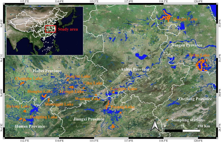
FIGURE 1. Locations of the study area and distribution of the sampling stations.

TABLE 1

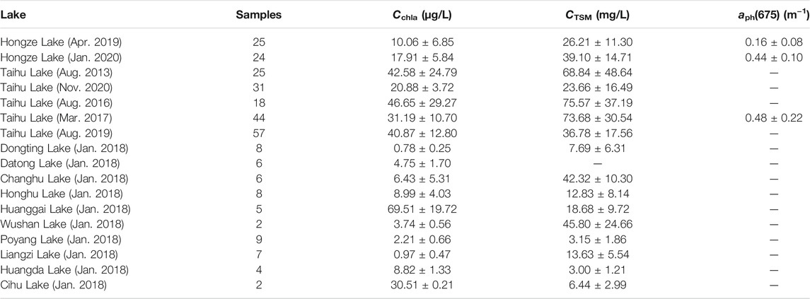
TABLE 1. Summary statistics of water parameters, including the concentrations of C_chla (μg/L), C_TSM (mg/L), and a_ph(675) (m⁻¹), of all 17 cruises.

The in-situ measured R_rs and C_chla were used for model calibration and validation. In-situ measured C_TSM was used to discuss the sensitivity of the models.

2.1.1 Measurement of R_rs

R_rs(λ) measurements were conducted by means of an ASD FieldSpec spectroradiometer, which has a spectral range of 350–1,050 nm at increment of 1.5 nm. The spectral resolution was interpolated into 1 nm after measurement. According to the above-water measurement method described in the Ocean Optical Protocols (Mueller et al., 2003), the above-water measurement method was used to measure the radiance spectra of the reference panel, water, and sky, respectively. At each site, ten spectra were collected, from which abnormal ones were eliminated and valid ones retained and averaged. Specific observation geometry was applied to effectively avoid the interference of a ship with the water surface and the influence of direct solar radiation during the measurement (Tang et al., 2004). Finally, R_rs(λ) was derived via the following equation (Tang et al., 2004; Le et al., 2009)

$\begin{array}{c}{\mathit{R}}_{\mathbf{r}\mathbf{s}}\left(\mathit{\lambda }\right)=\left({\mathit{L}}_{\mathbf{t}}-\mathit{r}\times {\mathit{L}}_{\mathbf{s}\mathbf{k}\mathbf{y}}\right)/\left({\mathit{L}}_{\mathbf{p}}\times \mathit{\pi }/{\mathit{\rho }}_{\mathbf{p}}\right)\end{array}(1)$

Where L_t is the total radiance received from the water surface; L_sky is the radiance from sky; L_p is the simultaneously observed radiance of the reference gray board. In this process, skylight reflectance at the air-water surface (r) was taken as 2.2% for calm weather, 2.5% for wind speed of up to 5 ms⁻¹, and 2.6–2.8% for wind speed of about 10 ms⁻¹ (Tang et al., 2004). The reflectance of the gray diffuse board (ρ_p) had been accurately corrected to be 30% in the factory, before we used it to carry out these field experiments.

2.1.2 Measurement of Water Constituents’ Concentration

Water samples were collected from the water surface (<20 cm) and kept in a cooler with ice. The fraction of each sample was used to measure concentrations of water constituents. Water samples were filtered through 0.7 μm Whatman GF/F glass fibre filters that had been combusted at 550°C for 4 h. The glass fibre filters were dried at 105°C for 4 h. C_TSM was obtained by measuring the difference in weights between combusted and dried glass fibre filters. Water samples for measuring C_chla were filtered with GF/C filters (Whatman). Chlorohphyll-a was extracted with ethanol (90%) at 80 °C for 6 h in darkness and then analyzed spectrophotometrically at 750 and 665 nm with a correction for phaeopigments using a spectrophotometer (Shimadzu UV-3600) (Chen et al., 2006).

2.1.3 Measurement of a_ph(λ)

The water samples were filtered and analyzed by a spectrophotometer (Shimadzu UV-3600) to obtain a_ph(λ) using the quantitative filter technique (Cleveland and Weidemann, 1993). First, the water samples were filtered through GF/C (Whatman) glass fibre filters to obtain TSM, and the absorbance of TSM was measured using a spectrophotometer. Pigments were removed from the water samples with NaClO and the water samples were refiltered to obtain tripton. The absorbance of tripton was obtained from these glfibre filters using a spectrophotometer. Data processing to calculate a_ph(λ) from the absorbance of tripton and TSM, respectively, was performed as described by Huang et al. (2011).

2.2 Satellite Data

Level-1b GOCI images covering Taihu Lake and Hongze Lake were downloaded from the Korea Ocean Satellite Centre (http://kosc.kordi.re.kr/). For the algorithm validation, the sampling times for the in-situ match-up data were ±0.5 h for the GOCI transit time. There were 40 match-up points (11 from Taihu Lake, Aug. 2013, five from Taihu Lake, Aug. 2019, 10 from Hongze Lake, Apr. 2019, and 14 from Hongze Lake, Nov. 2020) for GOCI images. These images were vector masked to remove land and islands after geometric correction. The GOCI atmospheric correction was carried out using an improved land target-based atmospheric correction method (Guanter et al., 2010; Liu et al., 2015).

2.3 Expanding of the TB Algorithm

The TB algorithm that developed by Dall’Olmo and Gitelson (Dall’olmo and Gitelson, 2005; Dall’olmo and Gitelson, 2006) is based on the following relationship between C_chla and R_rs:

$\begin{array}{c}{\mathit{C}}_{\mathbf{chla}}\propto \left[{\mathit{R}}_{\mathbf{r}\mathbf{s}}^{-\mathbf{1}}\left({\mathit{\lambda }}_{\mathbf{1}}\right)-{\mathit{R}}_{\mathbf{r}\mathbf{s}}^{-\mathbf{1}}\left({\mathit{\lambda }}_{\mathbf{2}}\right)\right]\times {\mathit{R}}_{\mathbf{r}\mathbf{s}}\left({\mathit{\lambda }}_{\mathbf{3}}\right)\end{array}(2)$

where R_rs is a function of the inherent absorption (a(λ)) and scattering (b_b(λ)) properties of the medium, according to the basic radiative transfer equation (Gordon et al., 1988).

$\begin{array}{c}{\mathit{R}}_{\mathit{r}\mathit{s}}\left(\mathit{\lambda }\right)=\frac{\mathit{f}\mathit{t}}{\mathit{Q}{\mathit{n}}^{\mathbf{2}}}\frac{{\mathit{b}}_{\mathbf{b}}\left(\mathit{\lambda }\right)}{\mathit{a}\left(\mathit{\lambda }\right)+{\mathit{b}}_{\mathbf{b}}\left(\mathit{\lambda }\right)}\end{array}(3)$

Absorption a(λ) can be separated into absorption related to a_ph, a_d, a_CDOM, and pure water (a_w), while b_b(λ) is the measurement of total backscattering. f/Q is depended on Sun zenith angle (Morel and Gentili, 1993), and can be approximated to be 0.0945 (Gordon et al., 1988), and t/n² = 0.54 (Austin, 1974; Clark, 1981).

The difference between the reciprocal reflectance R⁻¹(λ₁) and R⁻¹(λ₂) is approximated by

$\begin{array}{c}{\mathit{R}}_{\mathit{r}\mathit{s}}^{-\mathbf{1}}\left({\mathit{\lambda }}_{\mathbf{1}}\right)-{\mathit{R}}_{\mathit{r}\mathit{s}}^{-\mathbf{1}}\left({\mathit{\lambda }}_{\mathbf{2}}\right)\propto \frac{{\mathit{a}}_{\mathbf{p}\mathbf{h}}\left({\mathit{\lambda }}_{\mathbf{1}}\right)+{\mathit{a}}_{\mathbf{w}}\left({\mathit{\lambda }}_{\mathbf{1}}\right)-{\mathit{a}}_{\mathbf{w}}\left({\mathit{\lambda }}_{\mathbf{2}}\right)}{{\mathit{b}}_{\mathbf{b}}}\end{array}(4)$

based on the following assumptions: (a) b_b is spectrally invariant between λ₁ and λ₂; (b) a_ph(λ₁) >> a_ph(λ₂); (c) a_d(λ₁) + a_CDOM(λ₁) ≈ a_d(λ₂) + a_CDOM(λ₂).

Then, the third band, λ₃ is included to remove the effect of b_b. λ₃ is chosen to be in the near infrared (NIR) wavelengths, where reflectance by a_ph, a_d, and a_CDOM is minimal:

$\begin{array}{c}{\mathit{R}}_{\mathit{r}\mathit{s}}\left({\mathit{\lambda }}_{\mathbf{3}}\right)\propto \frac{{\mathit{b}}_{\mathbf{b}}\left({\mathit{\lambda }}_{\mathbf{3}}\right)}{\mathit{a}\left({\mathit{\lambda }}_{\mathbf{3}}\right)+{\mathit{b}}_{\mathbf{b}}\left({\mathit{\lambda }}_{\mathbf{3}}\right)}\approx \frac{{\mathit{b}}_{\mathbf{b}}}{{\mathit{a}}_{\mathbf{w}}\left({\mathit{\lambda }}_{\mathbf{3}}\right)}\propto {\mathit{b}}_{\mathbf{b}}\end{array}(5)$

The a_ph could be extracted by combining Eqs 4, 5:

$\begin{array}{c}\left[{\mathit{R}}_{\mathit{r}\mathit{s}}^{-\mathbf{1}}\left({\mathit{\lambda }}_{\mathbf{1}}\right)-{\mathit{R}}_{\mathit{r}\mathit{s}}^{-\mathbf{1}}\left({\mathit{\lambda }}_{\mathbf{2}}\right)\right]\times {\mathit{R}}_{\mathit{r}\mathit{s}}\left({\mathit{\lambda }}_{\mathbf{3}}\right)\propto {\mathit{C}}_{\mathbf{c}\mathbf{h}\mathbf{l}\mathbf{a}} \end{array}(6)$

Eq. 6 is the basic formula of the traditional TB algorithm, where λ₁ is in the spectral region in which chlorophyll-a shows maximum absorbance (λ₁ = 660–690 nm). λ₂ is in the spectral region in which chlorophyll-a shows minimum absorbance. The absorption of tripton and CDOM at λ₂ are very close to those at λ₁ (λ₂ = 700–730 nm). λ₃ is located in the spectral region such that R_rs(λ₃) is minimally affected by absorption of water constituents (λ₃ = 740–760 nm). Therefore, in multispectral sensors, only thin-band multispectral sensors like MERIS and S3 OLCI were widely used. According to the previous description, MERIS centre wavelengths for TB algorithm are λ₁ = 681nm, λ₂ = 708nm, and λ₃ = 753 nm. To simplify the discussion, Eq. 6 could be written as:

$\begin{array}{c}\left[{\mathit{R}}^{-\mathbf{1}}\left(\mathbf{681}\right)-{\mathit{R}}^{-\mathbf{1}}\left(\mathbf{708}\right)\right]\times \mathit{R}\left(\mathbf{753}\right)\propto {\mathit{C}}_{\mathbf{c}\mathbf{h}\mathbf{l}\mathbf{a}}\end{array}(7)$

According to some previous studies (Smyth et al., 2006; Chen et al., 2014), the ratio of absorption in different wavelength is fixed:

$\begin{array}{c}{\mathit{\epsilon }}_{\mathbf{a}}\left({\mathit{\lambda }}_{\mathbf{1}},{\mathit{\lambda }}_{\mathbf{2}}\right)=\mathit{a}\left({\mathit{\lambda }}_{\mathbf{1}}\right)/\mathit{a}\left({\mathit{\lambda }}_{\mathbf{2}}\right)\end{array}(8)$

What’s more, the GOCI band five is located in 660 nm (Table 1), which is nearby band 6 (680 nm). Then, the following equation can be established:

$\begin{array}{c}{\mathit{a}}_{\mathbf{p}\mathbf{h}}\left(\mathbf{680}\right)={\mathit{\epsilon }}_{\mathbf{a}\mathbf{p}\mathbf{h}}\left(\mathbf{680,660}\right)\times {\mathit{a}}_{\mathbf{p}\mathbf{h}}\left(\mathbf{660}\right)\end{array}(9)$

Therefore, the position of λ₂ in the standard TB algorithm could be moved from 710 to 660 nm to fit the GOCI band setting. Eq. 4 could be written as:

$\begin{array}{c}{\mathit{R}}^{-\mathbf{1}}\left(\mathbf{680}\right)-{\mathit{R}}^{-\mathbf{1}}\left(\mathbf{660}\right)\propto \frac{\left({\mathit{\epsilon }}_{\mathbf{a}\mathbf{p}\mathbf{h}}\left(\mathbf{680,660}\right)-\mathbf{1}\right)\times {\mathit{a}}_{\mathbf{p}\mathbf{h}}\left(\mathbf{660}\right)+{\mathit{a}}_{\mathbf{w}}\left(\mathbf{680}\right)-{\mathit{a}}_{\mathbf{w}}\left(\mathbf{660}\right)}{{\mathit{b}}_{\mathbf{b}}}\end{array}(10)$

Then, the expanded TB algorithm could be expressed as the following equation by combing Eq. 5 and Eq. 10 in the assumption that ε_aph(680,660) is fixed:

$\begin{array}{c}\left[{\mathit{R}}_{\mathit{r}\mathit{s}}^{-\mathbf{1}}\left(\mathbf{680}\right)-{\mathit{R}}_{\mathit{r}\mathit{s}}^{-\mathbf{1}}\left(\mathbf{660}\right)\right]\times {\mathit{R}}_{\mathit{r}\mathit{s}}\left(\mathbf{745}\right)\propto {\mathit{C}}_{\mathbf{c}\mathbf{h}\mathbf{l}\mathbf{a}}\end{array}(11)$

2.4 Accuracy Assessment

MAPE and RMSE were used to indicate errors in the estimated values, which could be calculated through the following equations:

$\begin{array}{c}\mathbf{R}\mathbf{M}\mathbf{S}\mathbf{E}=\sqrt{{\displaystyle \sum }_{\mathit{i}=\mathbf{1}}^{\mathit{n}}\left({\mathit{y}}_{\mathit{i}}-{\mathit{y}}_{\mathit{i}}^{\prime }\right)/\mathit{n}}\end{array}(12)$

$\begin{array}{c}\mathbf{M}\mathit{A}\mathbf{P}\mathbf{E}=\frac{\mathbf{1}}{\mathit{n}}{\displaystyle \sum }_{\mathit{i}=\mathbf{1}}^{\mathit{n}}\left|\frac{{\mathit{y}}_{\mathit{i}}-{\mathit{y}}_{\mathit{i}}^{\prime }}{{\mathit{y}}_{\mathit{i}}}\right|\end{array}(13)$

Where n is the number of samples; y_i is the measured value; y' i is the estimated value. In practical, MAPE indexes under different C_chla levels fluctuated dramatically. To better reflect the model performance, MAPE_low (only the samples that measured C_chla less than 10 μg/L were included) and MAPE_high (only the samples that measured C_chla greater or equal to 10 μg/L were included) were calculated separately.

2.5 Simulation Experiment

The main theoretical advantage of TB model is it will eliminate the optical influence of C_TSM in NIR spectral range. Therefore, we analyzed this influence based on a bio-optical model calibrated by Huang et al. (2011). In the bio-optical model, R_rs was expressed as a function of C_TSM, C_chla, and $a_{\text{CDOM}}\left({\lambda }_0\right)$ (Appendix A). To reveal the influence of C_TSM to C_chla estimation models, we simulated R_rs spectra between 400 and 800 nm under different C_chla and C_TSM combinations. C_chla and C_TSM were ranging from 1 μg/L to 200 μg/L, and 1 mg/L to 200 mg/L, respectively. $a_{\text{CDOM}}\left({\lambda }_0\right)$ was set to 0.5. Then, we defined a variable named model factor difference (Δ factor) to evaluate the stability of model factors to C_TSM. The expression of Δ factor is as follows:

$\begin{array}{c}{\mathit{\Delta }}_{\mathit{f}\mathit{a}\mathit{c}\mathit{t}\mathit{o}\mathit{r}}\left({\mathit{C}}_{\mathbf{c}\mathbf{h}\mathbf{l}\mathbf{a}},{\mathit{C}}_{\mathbf{T}\mathbf{S}\mathbf{M}}\right)=\mathit{f}\mathit{a}\mathit{c}\mathit{t}\mathit{o}\mathit{r}\left({\mathit{C}}_{\mathbf{c}\mathbf{h}\mathbf{l}\mathbf{a}},{\mathit{C}}_{\mathbf{T}\mathbf{S}\mathbf{M}}\right)-\mathit{f}\mathit{a}\mathit{c}\mathit{t}\mathit{o}\mathit{r}\left({\mathit{C}}_{\mathbf{c}\mathbf{h}\mathbf{l}\mathbf{a}},\mathbf{1}\right)\end{array}(14)$

where factor represents the three C_chla model factors, that is, MERIS TB (MTB) factor (i.e., [R^-1 rs(681)- R^-1 rs(708)] R_rs(753)), GOCI TB (GTB) (i.e., [R^-1 rs(680)- R^-1 rs(660)] R_rs(745)) factor, and GOCI BR (GBR) factor (i.e., R_rs(745)/R_rs(680)). All the factors were calculated from R_rs at a specific C_chla and C_TSM level. Δ factor represents the stability of the current factor to C_TSM. A Δ factor close to 0 means the current factor is not sensitive to C_TSM at the current C_chla level.

3 Results

3.1 R_rs Spectra Characteristics

The average R_rs (Figure 2A) of 15 cruises exhibited wide variability in terms of both magnitude and shape. Spectra of Wushan Lake and Cihu Lake were not plotted because we only collected two samples in these two lakes. This is inadequate to generate the correlation line. For eutrophicationic water, such as Huanggai Lake (Jan. 2018) and Taihu Lake (Aug. 2016), strong phytoplankton absorption formed the R_rs peaks around 570, 700, and 815nm, and the trough near 675 nm. For some other cruises such as Changhu Lake (Jan. 2018), its high turbidity and light eutrophication determined the stronger reflectance in red spectral range and weaker trough near 675 nm (Figure 2A). For relatively clean waters that contain less C_TSM and C_chla, like Liangzi Lake (Jan. 2018), the average R_rs curve have small magnitude and weak phytoplankton characters in red and NIR spectral ranges.

FIGURE 2

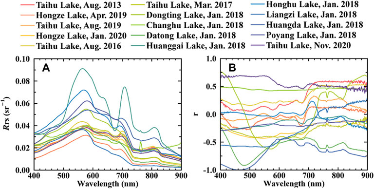
FIGURE 2. Average spectrum of 17 cruises (A) and the correlation coefficients between C_chla and Rrs (λ) (B) in the spectral range of 400–900 nm.

The correlation coefficients between R_rs and C_chla at each wavelength (Figure 2B) also indicated the complexity of the samples. Datasets with significant trough at 680 nm and peak at 700 nm exhibited similar correlation curves. However, for lakes with high turbidity and low eutrophication level, like Changhu Lake, the correlation line looks flat: peak in 700 nm disappeared because high turbidity weakened the R_rs sensitivity to C_chla.

In conclusion, the complex optical properties of inland water require a C_chla estimation model that could eliminate the optical influence of other water color constituents, especially C_TSM.

3.2 a_ph Spectra Characteristics

The average a_ph spectrum (Figure 3) contains three peaks. The first one is at 440 nm, which is caused by chlorophyll-a, chlorophyll-b, chlorophyll-c, carotenoid, and other accessory pigments. The second peak at 625 nm is caused by phycocyanin. The last one around 675 nm is mainly caused by the absorption of chlorophyll-a (Haardt and Maske, 1987; Dekker, 1993).

FIGURE 3

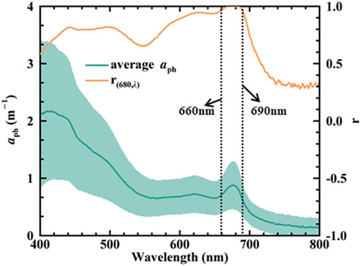
FIGURE 3. Average a_ph spectral and the correlation coefficients between a_ph(λ) and a_ph(680) [r_(680,λ) in the figure] in the spectral range of 400–800 nm.

In order to investigate the rationality of the core assumption of the GOCI TB model, i.e., the stability of ε_aph, we calculated linear correlation coefficients between a_ph at 680 nm and other spectral bands (i.e., line r _{(680, λ)} in Figure 3). Overall, the r_{(680, λ)} line had a similar shape with the average a_ph line. This means the main factor that affects inter-band correlation of a_ph is its magnitude. In detail, the correlationship became stronger in the spectral range from 400 to 500 nm. Then, a trough appears in 550 nm. In the wavelength range between 600 and 690 nm, r_{(680, λ)} is entirety greater than 0.9. The strongest correlation appears in 660–690 nm, where the r _{(680, λ)} line is above 0.98. For the bands beyond 690 nm, with the increasing of wavelength, the correlation coefficients rapidly decrease together with the a_ph spectrum.

The relationship between a_ph(660) and a_ph(680) (Figure 4) of all the available in-situ samples denote that when the intercept is set to 0, the linear fitting R² is 0.965. This means a_ph(660) can explain more than 96% changes of a_ph(680) in our dataset. Therefore, the assumption in Eq. 9, i.e., ε_aph(680,660) is fixed, is considered to be reasonable in this study (ε_aph(680,660) = 1.23).

FIGURE 4

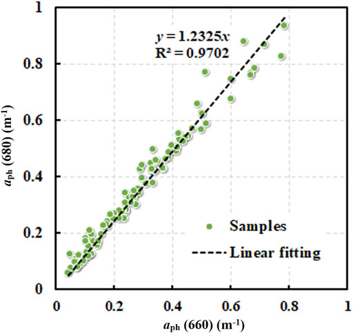
FIGURE 4. Scatter plot of a_ph(660) and a_ph(680).

3.3 Calibration and Validation of the Models

Three algorithms were calibrated and validated in this study, they are: MERIS TB algorithm (based on Eq. 7), GOCI TB algorithm (based on Eq. 11), and GOCI BR algorithm R_rs(745)/R_rs(680) (Huang et al., 2014; Bao et al., 2015) was selected as the model factor. The whole in-situ dataset was randomly separated into 188 calibration samples and 93 validation samples. The parameters of the three models were determined in the calibration dataset by a simple linear fitting method (Figures 5A,C,E). Their expressions are as follows:

$\begin{array}{c}{\mathit{C}}_{\mathbf{c}\mathbf{h}\mathbf{l}\mathbf{a}}=\mathbf{260.850}\times \left[{\mathit{R}}_{\mathbf{r}\mathbf{s}}^{-\mathbf{1}}\left(\mathbf{681}\right)-{\mathit{R}}_{\mathbf{r}\mathbf{s}}^{-\mathbf{1}}\left(\mathbf{708}\right)\right]{\mathit{R}}_{\mathbf{r}\mathbf{s}}\left(\mathbf{753}\right)+\mathbf{26.342} ({\mathit{R}}^{\mathbf{2}}=\mathbf{0.878}, \mathit{P}<\mathbf{0.001})\end{array}(15)$

$\begin{array}{c}{\mathit{C}}_{\mathbf{c}\mathbf{h}\mathbf{l}\mathbf{a}}=\mathbf{763.230}\times \left[{\mathit{R}}_{\mathbf{r}\mathbf{s}}^{-\mathbf{1}}\left(\mathbf{680}\right)-{\mathit{R}}_{\mathbf{r}\mathbf{s}}^{-\mathbf{1}}\left(\mathbf{660}\right)\right]{\mathit{R}}_{\mathbf{r}\mathbf{s}}\left(\mathbf{745}\right)-\mathbf{4.485} \left({\mathit{R}}^{\mathbf{2}}=\mathbf{0.823}, \mathit{P}<\mathbf{0.001}\right)\end{array}(16)$

$\begin{array}{c}{\mathit{C}}_{\mathbf{c}\mathbf{h}\mathbf{l}\mathbf{a}}=\mathbf{127.940}\times \frac{{\mathit{R}}_{\mathbf{r}\mathbf{s}}\left(\mathbf{745}\right)}{{\mathit{R}}_{\mathbf{r}\mathbf{s}}\left(\mathbf{680}\right)}-\mathbf{35.436} \left({\mathit{R}}^{\mathbf{2}}=\mathbf{0.569}, \mathit{P}<\mathbf{0.001}\right)\end{array}(17)$

FIGURE 5

FIGURE 5. Scatter plot of (A) MERIS TB model; (C) GOCI TB model; (E) GOCI BR model, and the validation result of (B) MERIS TB model; (D) GOCI TB model; (F) GOCI BR model.

In the validation dataset, RMSE of the MERIS TB, GOCI TB, and GOCI BR models are 12.943 μg/L, 13.313 μg/L, and 22.613 μg/L, respectively. MAPE_low samples are 8.089, 7.725, and 29.898, respectively. MAPE_high are 0.433, 0.463, and 0.915, respectively (Figures 5B,D,F). The results indicated that GOCI TB algorithm performs better than GOCI BR algorithm and similar with MERIS TB algorithm. Wavelengths in the brackets represent specific band centers of MERIS and GOCI.

3.4 Performance in Match-Up Samples

Table 2 shows the atmospheric correction results of the 40 match-up points. The average MAPE and RMSE over all spectral bands are 0.216 and 4.578 × 10⁻³, respectively. Generally, the atmospheric correction yields satisfactory accuracy, especially for red and NIR bands.

TABLE 2

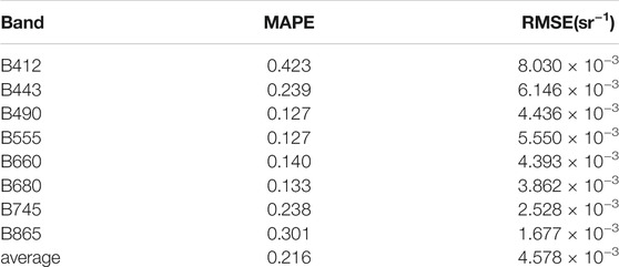
TABLE 2. Atmospheric correction errors.

The C_chla estimation results from GOCI TB and BR models represent that, generally, the performance of the two models are similar with those of in-situ dataset (Figure 5). RMSE of BR and TB models are 12.42 μg/L and 9.90 μg/L, respectively. This means that GOCI TB model improved the accuracy for about 25%. MAPE of BR and TB models are 0.94 and 0.60, respectively. The improvement was about 56%. This suggesting that the GOCI TB model could improve more estimation accuracy in low C_chla conditions.

3.5 C_chla Maps

We applied GOCI TB and BR models to the preprocessed GOCI images and yielded the C_chla maps (Figure 6). Generally, the GOCI TB and GOCI BR C_chla maps have similar spatial distribution: high C_chla values appeared in Zhushan Bay, Meiliang Bay, north of Gonghu Bay, and south west lake. Low C_chla region distributed in the center lake. Notably, an opposite trend appeared between GOCI TB C_chla series and GOCI BR C_chla series: from 8:30 to 15:30, C_chla is getting larger in GOCI TB C_chla maps and smaller in the GOCI BR yielded ones.

FIGURE 6

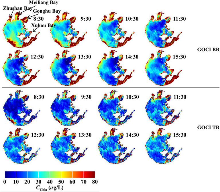
FIGURE 6. C_chla maps that yielded by BR and TB algorithm using GOCI image in 13 May 2013.

4 Discussion

4.1 Error Distribution Analysis

TB model can eliminate the optical influence of total suspended matter in NIR spectral range. To visualize this elimination, MAPE of each sample was calculated for all the three models and plotted in the C_chla-C_TSM space (Figure 7). The results indicated that, generally, MERIS TB and GOCI TB have similar MAPE distribution. GOCI TB algorithm performs slightly better in low C_chla (C_chla < 10 μg/L), high C_TSM (C_TSM > 30 mg/L) region, where GOCI BR result exhibits significant error (Figure 5E and Figure 7C).

FIGURE 7

FIGURE 7. Scatter plot of the MAPE versus C_TSM and C_chla of (A) MERIS TB model; (B) GOCI TB model; (C) GOCI BR model. The vertical and horizontal histograms in each plot represent the concentration distributions of C_chla and C_TSM, respectively.

To understand the failure of the GOCI BR algorithm in low C_chla, high C_TSM condition, we carried out a further analysis. Based on GOCI band settings, the linear correlation coefficients of BR factor with both C_chla and C_TSM were calculated (Figure 8). What interesting is, the correlation map of C_TSM has a similar distribution with that of C_chla. Even the overall correlation coefficients of C_TSM are lower than C_chla, the significant correlation between BR factors and C_TSM at 680, 745, and 865 nm indicated the unneglectable influence of suspended matter in BR model. Meanwhile, the correlation coefficients between GOCI TB factors and C_TSM was 0.286, which is obviously lower than that of BR factors (higher than 0.5 in Figure 8B). This comparison suggesting that compared with GOCI BR factor, GOCI TB factor could effectively eliminate the impact of TSM and yield a more reliable C_chla estimation result.

FIGURE 8

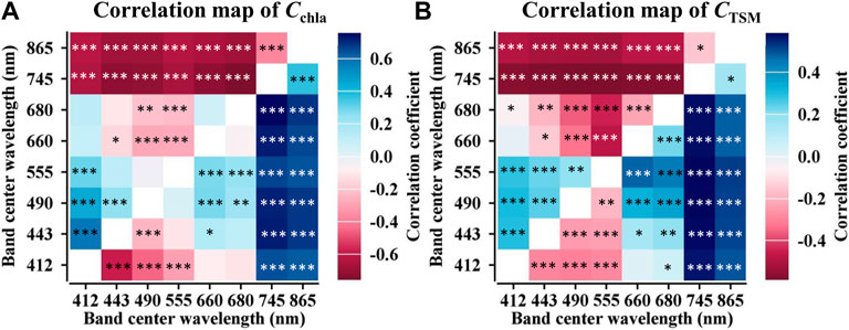
FIGURE 8. Correlation maps of GOCI BR factors to (A) C_chla and (B) C_TSM. Marks “*”, “**”, and “***” represent for p value less than 0.05, 0.01, and 0.001, respectively.

4.2 Theoretical Analysis of the Model Sensitivity to C_TSM

The simulation experiment results will be discussed as follows: For each C_chla level, we calculated ${\Delta }_{factor}$ under all C_TSM conditions to yield a sensitivity line in Figure 9. For an ideal factor that could completely erase the impact of C_TSM, the sensitivity line will be y = 0 (the dashed lines in Figure 9), which means no matter how much TSM is in the water, the spectral factor kept the same. Therefore, the distance of ${\Delta }_{factor}$ line to the dashed line reflects the stability of the current factor.

FIGURE 9

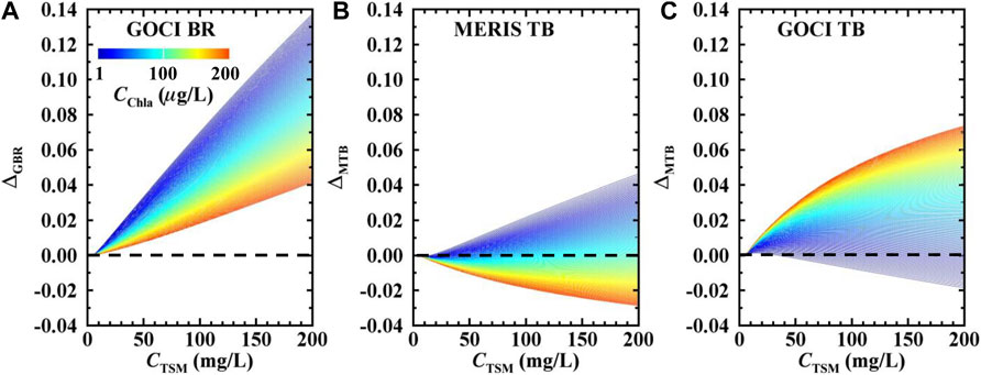
FIGURE 9. Sensitivity simulation result of (A) GOCI BR model, (B) MERIS TB model, and (C) GOCI TB model in different C_TSM and C_chla conditions.

The results (Figure 9) indicated that the three factors have different stable C_chla ranges. Generally, the influence of TSM to C_chla spectra factors are increasing together with C_TSM. However, For MERIS TB factor, the most stable C_chla range is about 70 μg/L (Figure 9B). High C_chla sensitivity and low C_chla sensitivity lines equally distributed around the dashed line. GOCI TB factor is insensitive to C_TSM when C_chla is smaller than 40 μg/L (Figure 9C). With the increasing of C_TSM, offset of the high C_chla sensitivity line became larger. Δ GBR has a linear relationship with C_TSM. For lower C_chla, the factor difference is higher, which indicates that the GOCI BR factor is unstable in low C_chla conditions.

In conclusion, the MERIS TB and GOCI TB factors perform similar: they both have stable C_chla ranges, which are around 76 μg/L and less than 40 μg/L, respectively. GOCI BR algorithm did not show a stable region: with the increasing of C_TSM, the factor became more and more sensitive to TSM. The simulation results can partly explain the model performances in section 4.1.

4.3 Comparison of C_chla Maps Yielded From GOCI TB and BR Models

Water constituents time series of specific water body has been widely reported (Le et al., 2013; Feng et al., 2014; Palmer et al., 2015). Meanwhile, we proved that different models have different performance under varied conditions (section 3.4). Then, how will this difference affect the spatial-temporal distribution of C_chla maps? To answer this question, we calculated the correlation coefficients between GOCI TB and BR yielded C_chla maps pixel by pixel (Figure 10A). A positive correlation coefficient denotes that C_chla yielded from TB and BR algorithms have similar temporal changes, and vice versa. The results indicated that in high C_chla regions, like Zhushan Bay, Meiliang Bay, Gonghu Bay, and south west lake, two map series showed strong consistency. The correlation coefficients are generally higher than 0.8. However, a large negative correlation region in the center lake means that the two series have totally opposite C_chla trends in this region. C_TSM sensitivity discussed in section 4.2 can explain this phenomenon: resuspention in the center lake increased C_TSM and the instability of GOCI BR model. The histogram of correlation coefficient map (Figure 11B) demonstrated that the two models yielded opposite trends in a considerable region of Taihu Lake. This will definitely influence the statistical analysis in long-term water C_chla monitoring missions.

FIGURE 10

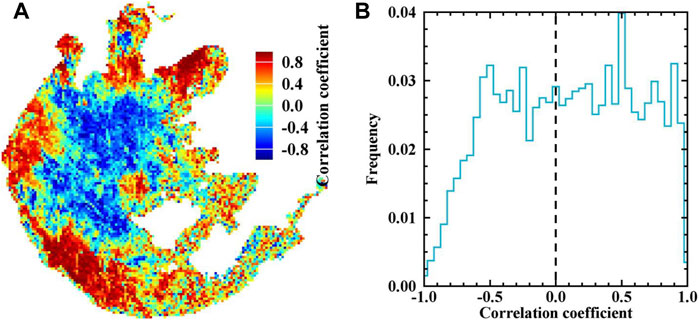
FIGURE 10. Time series correlation coefficients between TB model and BR yielded C_chla maps (A), and its probability density plot (B).

FIGURE 11

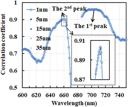
FIGURE 11. Correlation coefficients of GOCI TB factors to C_chla.

4.4 Influence of Position and Width of Band λ₂ to GOCI TB Model

Our expansion to the TB model is focusing on λ₂. Following the original ideal of the TB model, we analyzed the effect of band λ₂ to the GOCI TB model by calculating the band-by-band correlation coefficients between C_chla and GOCI TB factor.

We fixed the positions of λ₁ and λ₃ and changed band λ₂ from 600 to 740 nm to yield the correlation coefficient line (Figure 11). The widest and highest correlation peak (the first peak in Figure 11) appears at around 710nm, where is close to the theoretical optimal band position in previous researches (Dall’olmo and Gitelson, 2005; Le et al., 2011). Therefore, the first peak is the best choice when the sensor could provide proper spectral bands. It is also worth noting that the second peak exists at around 660 nm (Figure 11). In fact, this peak had been reported by Dall’olmo and Gitelson, 2005 and Le et al. (2009) researches. This suggesting that 660 nm is always a potential selection for TB models.

To further discuss the impact of bandwidth to the GOCI TB model, we resampled R_rs (660) to 5, 15, 25, and 35 nm width, respectively. Then, we calculated the GOCI TB factor based on the resampled R_rs (660) and their correlation coefficients with C_chla (Figure 11). The result denoted that, even the bandwidth was set to 35 nm, the GOCI TB factor still have high correlation coefficient with C_chla (larger than 0.87). This means that the GOCI TB factor is not sensitive to the width of band λ₂.

4.5 Potential of the Expanded TB Algorithm

An obstacle of applying traditional TB algorithm is band λ₂, which located in range of 690–710 nm (Dall’olmo and Gitelson, 2005; Dall’olmo and Gitelson, 2006). By a strict theoretical derivation, the expanded TB model suggests that when the sensor set no bands in 690–710 nm, λ₂ can be moved to 660–690 nm. The expanded TB algorithm has both clear mechanism and satisfactory performance. In fact, apart from GOCI, the proposed model can be also applied to multispectral sensors like S2 MSI, MODIS (onboard the Terra/Aqua satellite), and VIIRS (onboard the National Polar-orbiting Partnership satellite) (Figure 12).

FIGURE 12

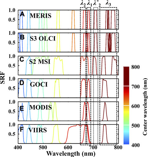
FIGURE 12. Band settings of (A) MERIS, (B) S3 OLCI, (C) S2 MSI, (D) GOCI, (E) MODIS, (F) VIIRS (λ*₂ and λ₂ represents the second band of the original TB and expanded TB models).

Therefore, for MODIS (250/500 m band settings), VIIRS, and S2 MSI, their TB and best-fitted BR models were calibrated using the in-situ dataset (Table 3). In general, all the sensors perform better using TB model. Especially for MODIS and S2 MSI. For MODIS, compared with BR model, the TB model decreased the RMSE, MAPE_low and MAPE_high by 24.70%, 29.76%, and 17.77%. These reductions for S2 MSI are 25.62%, 30.48%, and 16.50%, respectively. For VIIRS, the band width of λ₂ is so broad (Figure 12) that it is partly out of the second high correlation peak (Figure 11). Even though, TB model still improved the performance slightly.

TABLE 3

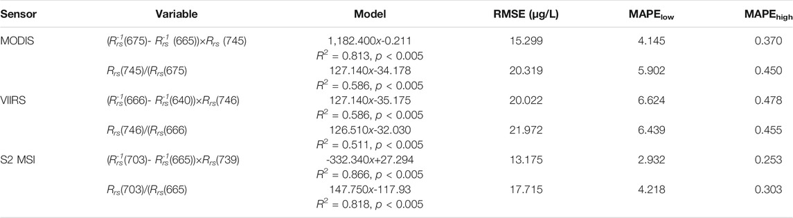
TABLE 3. TB and BR models for MODIS, VIIRS, and S2

Conclusively, the expanded TB algorithm provides a wider choice for accurately monitoring inland complex water.

5 Conclusion

In this research, the TB algorithm is expanded for GOCI image to remotely estimate C_chla for optically complex water. The GOCI TB model was calibrated and validated by a comprehensive in-situ measured dataset and GOCI images. By comparing with MERIS TB and GOCI BR algorithms, the following conclusions can be drawn:

1) In the expanded TB algorithm, λ₂ is located in the spectral range between 680 and 700 nm or 660–680 nm. The core assumption of the expanded TB algorithm is reasonable. The validation result indicated that GOCI TB algorithm have similar accuracy with MERIS TB algorithm.

2) In highly turbid waters, GOCI BR factor cannot explain the change of C_chla. Meanwhile, the GOCI TB algorithm successfully eliminates $b_{\text{b}}$ at NIR spectral range and performs well in high C_TSM conditions.

3) Compared with the BR algorithm, GOCI TB algorithm can yield more reasonable C_chla map for water environment monitoring and analyzing.

4) The expanded TB algorithm is proper for other multispectral sensors like S2 MSI, MODIS, and VIIRS. It provides wider choice for the future inland water remote monitoring missions.

Data Availability Statement

The original contributions presented in the study are included in the article/Supplementary Material, further inquiries can be directed to the corresponding author.

Author Contributions

YG performed the data and analysis. YG and CH wrote the paper. CH designed the research. YL, CD, and YL helped to design the experiments. WC contributed to the model development. LS and GJ helped to refine the algorithm.

Funding

This work is supported by National Natural Science Foundation of China (grant #: 41971286, 41701422, 42001296, 42071333) and Natural Science Foundation of Jiangsu Province (grant number BK20191058).

Conflict of Interest

The authors declare that the research was conducted in the absence of any commercial or financial relationships that could be construed as a potential conflict of interest.

Publisher’s Note

All claims expressed in this article are solely those of the authors and do not necessarily represent those of their affiliated organizations, or those of the publisher, the editors and the reviewers. Any product that may be evaluated in this article, or claim that may be made by its manufacturer, is not guaranteed or endorsed by the publisher.

References

Augusto-Silva, P., Ogashawara, I., Barbosa, C., De Carvalho, L., Jorge, D., Fornari, C., et al. (2014). Analysis of MERIS Reflectance Algorithms for Estimating Chlorophyll-A Concentration in a Brazilian Reservoir. Remote Sensing 6, 11689–11707. doi:10.3390/rs61211689

CrossRef Full Text | Google Scholar

Austin, R. (1974). Inherent Spectral Radiance Signatures of the Ocean Surface. Ocean color Anal. 7410, 1–20.

Google Scholar

Bao, Y., Tian, Q., and Chen, M. (2015). A Weighted Algorithm Based on Normalized Mutual Information for Estimating the Chlorophyll-A Concentration in Inland Waters Using Geostationary Ocean Color Imager (GOCI) Data. Remote Sensing 7, 11731–11752. doi:10.3390/rs70911731

CrossRef Full Text | Google Scholar

Bresciani, M., Stroppiana, D., Odermatt, D., Morabito, G., and Giardino, C. (2011). Assessing Remotely Sensed Chlorophyll-A for the Implementation of the Water Framework Directive in European Perialpine Lakes. Sci. Total Environ. 409, 3083–3091. doi:10.1016/j.scitotenv.2011.05.001

PubMed Abstract | CrossRef Full Text | Google Scholar

Chen, J., Cui, T., Qiu, Z., and Lin, C. (2014). A Three-Band Semi-analytical Model for Deriving Total Suspended Sediment Concentration from HJ-1A/CCD Data in Turbid Coastal Waters. ISPRS J. Photogrammetry Remote Sensing 93, 1–13. doi:10.1016/j.isprsjprs.2014.02.011

CrossRef Full Text | Google Scholar

Chen, J., Quan, W., Wen, Z., and Cui, T. (2013). An Improved Three-Band Semi-analytical Algorithm for Estimating Chlorophyll-A Concentration in Highly Turbid Coastal Waters: a Case Study of the Yellow River Estuary, China. Environ. Earth Sci. 69, 2709–2719. doi:10.1007/s12665-012-2093-1

CrossRef Full Text | Google Scholar

Chen, Y., Chen, K., and Hu, Y. (2006). Discussion on Possible Error for Phytoplankton Chlorophyll-A Concentration Analysis Using Hot-Ethanol Extraction Method. J. Lake Sci. 18, 550–552.

Google Scholar

Clark, D. K. (1981). “Phytoplankton Pigment Algorithms for the Nimbus-7 CZCS,” in Oceanography from Space (Springer), 227–237. doi:10.1007/978-1-4613-3315-9_28

CrossRef Full Text | Google Scholar

Cleveland, J. S., and Weidemann, A. D. (1993). Quantifying Absorption by Aquatic Particles: A Multiple Scattering Correction for Glass-Fiber Filters. Limnol. Oceanogr. 38, 1321–1327. doi:10.4319/lo.1993.38.6.1321

CrossRef Full Text | Google Scholar

Dall'olmo, G., and Gitelson, A. A. (2005). Effect of Bio-Optical Parameter Variability on the Remote Estimation of Chlorophyll-A Concentration in Turbid Productive Waters: Experimental Results. Appl. Opt. 44, 412–422. doi:10.1364/ao.44.000412

PubMed Abstract | CrossRef Full Text | Google Scholar

Dall'olmo, G., and Gitelson, A. A. (2006). Effect of Bio-Optical Parameter Variability and Uncertainties in Reflectance Measurements on the Remote Estimation of Chlorophyll-A Concentration in Turbid Productive Waters: Modeling Results. Appl. Opt. 45, 3577–3592. doi:10.1364/ao.45.003577

PubMed Abstract | CrossRef Full Text | Google Scholar

Dekker, A. G. (1993). Detection of Optical Water Quality Parameters for Eutrophic Waters by High Resolution Remote Sensing.

Google Scholar

Duan, H., Ma, R., Zhang, Y., Loiselle, S. A., Xu, J., Zhao, C., et al. (2010). A New Three-Band Algorithm for Estimating Chlorophyll Concentrations in Turbid Inland Lakes. Environ. Res. Lett. 5, 044009. doi:10.1088/1748-9326/5/4/044009

CrossRef Full Text | Google Scholar

Feng, L., Hu, C., Han, X., Chen, X., and Qi, L. (2014). Long-Term Distribution Patterns of Chlorophyll-A Concentration in China's Largest Freshwater Lake: MERIS Full-Resolution Observations with a Practical Approach. Remote Sensing 7, 275–299. doi:10.3390/rs70100275

CrossRef Full Text | Google Scholar

Gitelson, A. A., Schalles, J. F., and Hladik, C. M. (2007). Remote Chlorophyll-A Retrieval in Turbid, Productive Estuaries: Chesapeake Bay Case Study. Remote Sensing Environ. 109, 464–472. doi:10.1016/j.rse.2007.01.016

CrossRef Full Text | Google Scholar

Gordon, H. R., Brown, O. B., Evans, R. H., Brown, J. W., Smith, R. C., Baker, K. S., et al. (1988). A Semianalytic Radiance Model of Ocean Color. J. Geophys. Res. 93, 10909–10924. doi:10.1029/jd093id09p10909

CrossRef Full Text | Google Scholar

Guanter, L., Ruiz-Verdú, A., Odermatt, D., Giardino, C., Simis, S., Estellés, V., et al. (2010). Atmospheric Correction of ENVISAT/MERIS Data over Inland Waters: Validation for European Lakes. Remote Sensing Environ. 114, 467–480. doi:10.1016/j.rse.2009.10.004

CrossRef Full Text | Google Scholar

Guo, Y., Huang, C., Zhang, Y., Li, Y., and Chen, W. (2020). A Novel Multitemporal Image-Fusion Algorithm: Method and Application to GOCI and Himawari Images for Inland Water Remote Sensing. IEEE Trans. Geosci. Remote Sensing 58, 4018–4032. doi:10.1109/tgrs.2019.2960322

CrossRef Full Text | Google Scholar

Gurlin, D., Gitelson, A. A., and Moses, W. J. (2011). Remote Estimation of Chl-A Concentration in Turbid Productive Waters - Return to a Simple Two-Band NIR-Red Model? Remote Sensing Environ. 115, 3479–3490. doi:10.1016/j.rse.2011.08.011

CrossRef Full Text | Google Scholar

Haardt, H., and Maske, H. (1987). Specific In Vivo Absorption Coefficient of Chlorophyll a at 675 Nm1. Limnol. Oceanogr. 32, 608–619. doi:10.4319/lo.1987.32.3.0608

CrossRef Full Text | Google Scholar

Honeywill, C., Paterson, D., and Hagerthey, S. (2002). Determination of Microphytobenthic Biomass Using Pulse-Amplitude Modulated Minimum Fluorescence. Eur. J. Phycology 37, 485–492. doi:10.1017/s0967026202003888

CrossRef Full Text | Google Scholar

Huang, C.-C., Li, Y.-M., Sun, D.-Y., and Le, C.-F. (2011). Retrieval of Microcystis Aentginosa Percentage from High Turbid and Eutrophia Inland Water: A Case Study in Taihu Lake. IEEE Trans. Geosci. Remote Sensing 49, 4090–4100. doi:10.1109/tgrs.2011.2129521

CrossRef Full Text | Google Scholar

Huang, C., Guo, Y., Yang, H., Li, Y., Zou, J., Zhang, M., et al. (2015a). Using Remote Sensing to Track Variation in Phosphorus and its Interaction with Chlorophyll-A and Suspended Sediment. IEEE J. Sel. Top. Appl. Earth Observations Remote Sensing 8, 4171–4180. doi:10.1109/jstars.2015.2438293

CrossRef Full Text | Google Scholar

Huang, C., Shi, K., Yang, H., Li, Y., Zhu, A.-X., Sun, D., et al. (2015b). Satellite Observation of Hourly Dynamic Characteristics of Algae with Geostationary Ocean Color Imager (GOCI) Data in Lake Taihu. Remote Sensing Environ. 159, 278–287. doi:10.1016/j.rse.2014.12.016

CrossRef Full Text | Google Scholar

Huang, C., Zou, J., Li, Y., Yang, H., Shi, K., Li, J., et al. (2014). Assessment of NIR-Red Algorithms for Observation of Chlorophyll-A in Highly Turbid Inland Waters in China. ISPRS J. Photogrammetry Remote Sensing 93, 29–39. doi:10.1016/j.isprsjprs.2014.03.012

CrossRef Full Text | Google Scholar

Kravitz, J., Matthews, M., Bernard, S., and Griffith, D. (2019). Application of Sentinel 3 OLCI for Chl-A Retrieval over Small Inland Water Targets: Successes and Challenges. Remote Sensing Environ. 237.

Google Scholar

Kutser, T. (2004). Quantitative Detection of Chlorophyll in Cyanobacterial Blooms by Satellite Remote Sensing. Limnol. Oceanogr. 49, 2179–2189. doi:10.4319/lo.2004.49.6.2179

CrossRef Full Text | Google Scholar

Le, C., Hu, C., English, D., Cannizzaro, J., Chen, Z., Feng, L., et al. (2013). Towards a Long-Term Chlorophyll-A Data Record in a Turbid Estuary Using MODIS Observations. Prog. Oceanography 109, 90–103. doi:10.1016/j.pocean.2012.10.002

CrossRef Full Text | Google Scholar

Le, C., Li, Y., Zha, Y., Sun, D., Huang, C., and Lu, H. (2009). A Four-Band Semi-analytical Model for Estimating Chlorophyll a in Highly Turbid Lakes: The Case of Taihu Lake, China. Remote Sensing Environ. 113, 1175–1182. doi:10.1016/j.rse.2009.02.005

CrossRef Full Text | Google Scholar

Le, C., Li, Y., Zha, Y., Sun, D., Huang, C., and Zhang, H. (2011). Remote Estimation of Chlorophyll a in Optically Complex Waters Based on Optical Classification. Remote Sensing Environ. 115, 725–737. doi:10.1016/j.rse.2010.10.014

CrossRef Full Text | Google Scholar

Lee, Z., Lance, V. P., Shang, S., Vaillancourt, R., Freeman, S., Lubac, B., et al. (2011). An Assessment of Optical Properties and Primary Production Derived from Remote Sensing in the Southern Ocean (SO GasEx). J. Geophys. Res. Oceans 116, 1978–2012. doi:10.1029/2010jc006747

CrossRef Full Text | Google Scholar

Li, J. (2007). Study of Retrieval of Inland Water Quality Parameters from Hyperspectral Remote Sensing Data by Analytical Approach – Taking Taihu Lake as an Example [doctor’s Thesis]. [Beijing: Institute of Remote Sensing Application, Chinese Academy of Sciences.

Google Scholar

Li, Y., Huang, J., Wei, Y., and Lu, W. (2006). Inversing Chlorophyll Concentration of Taihu Lake by Analytic Model. J. Remote Sensing 10, 169–175.

Google Scholar

Liu, G., Li, L., Song, K., Li, Y., Lyu, H., Wen, Z., et al. (2020). An OLCI-Based Algorithm for Semi-empirically Partitioning Absorption Coefficient and Estimating Chlorophyll a Concentration in Various Turbid Case-2 Waters. Remote Sensing Environ. 239, 111648. doi:10.1016/j.rse.2020.111648

CrossRef Full Text | Google Scholar

Liu, G., Li, Y., Lyu, H., Wang, S., Du, C., and Huang, C. (2015). An Improved Land Target-Based Atmospheric Correction Method for Lake Taihu. IEEE J. Selected Top. Appl. Earth Observations Remote Sensing 9, 793–803.

Google Scholar

Morel, A., and Gentili, B. (1993). Diffuse Reflectance of Oceanic Waters II Bidirectional Aspects. Appl. Opt. 32, 6864–6879. doi:10.1364/ao.32.006864

PubMed Abstract | CrossRef Full Text | Google Scholar

Moses, W. J., Gitelson, A. A., Berdnikov, S., Bowles, J. H., Povazhnyi, V., Saprygin, V., et al. (2014). HICO-based NIR–Red Models for Estimating Chlorophyll-Concentration in Productive Coastal Waters.

Google Scholar

Moses, W. J., Gitelson, A. A., Perk, R. L., Gurlin, D., Rundquist, D. C., Leavitt, B. C., et al. (2012). Estimation of Chlorophyll-A Concentration in Turbid Productive Waters Using Airborne Hyperspectral Data. Water Res. 46, 993–1004. doi:10.1016/j.watres.2011.11.068

PubMed Abstract | CrossRef Full Text | Google Scholar

Mueller, J. L., Morel, A., Frouin, R., Davis, C., Arnone, R., Carder, K., et al. (2003). Ocean Optics Protocols for Satellite Ocean Color Sensor Validation, Revision 4. Volume III: Radiometric Measurements and Data Analysis Protocols.

Google Scholar

Neil, C., Spyrakos, E., Hunter, P. D., and Tyler, A. N. (2019). A Global Approach for Chlorophyll-A Retrieval across Optically Complex Inland Waters Based on Optical Water Types. Remote Sensing Environ. 229, 159–178. doi:10.1016/j.rse.2019.04.027

CrossRef Full Text | Google Scholar

Palmer, S. C. J., Odermatt, D., Hunter, P. D., Brockmann, C., Présing, M., Balzter, H., et al. (2015). Satellite Remote Sensing of Phytoplankton Phenology in Lake Balaton Using 10years of MERIS Observations. Remote Sensing Environ. 158, 441–452. doi:10.1016/j.rse.2014.11.021

CrossRef Full Text | Google Scholar

Shi, K., Li, Y., Li, L., Lu, H., Song, K., Liu, Z., et al. (2013). Remote Chlorophyll-A Estimates for Inland Waters Based on a Cluster-Based Classification. Sci. Total Environ. 444, 1–15. doi:10.1016/j.scitotenv.2012.11.058

PubMed Abstract | CrossRef Full Text | Google Scholar

Smyth, T. J., Moore, G. F., Hirata, T., and Aiken, J. (2006). Semianalytical Model for the Derivation of Ocean Color Inherent Optical Properties: Description, Implementation, and Performance Assessment. Appl. Opt. 45, 8116–8131. doi:10.1364/ao.45.008116

PubMed Abstract | CrossRef Full Text | Google Scholar

Tang, J., Tian, G., Wang, X., Wang, X., and Song, Q. (2004). The Method of Water Spectra Measurement and Analysis Ⅰ: Above-Water Method. J. Remote Sens ing 8, 37–44.

Google Scholar

Xu, J., Li, F., Zhang, B., Song, K., Wang, Z., Liu, D., et al. (2009). Estimation of Chlorophyll-A Concentration Using Field Spectral Data: a Case Study in Inland Case-II Waters, North China. Environ. Monit. Assess. 158, 105–116. doi:10.1007/s10661-008-0568-z

PubMed Abstract | CrossRef Full Text | Google Scholar

Yacobi, Y. Z., Moses, W. J., Kaganovsky, S., Sulimani, B., Leavitt, B. C., and Gitelson, A. A. (2011). NIR-red Reflectance-Based Algorithms for Chlorophyll-A Estimation in Mesotrophic Inland and Coastal Waters: Lake Kinneret Case Study. Water Res. 45, 2428–2436. doi:10.1016/j.watres.2011.02.002

PubMed Abstract | CrossRef Full Text | Google Scholar

Yang, W., Matsushita, B., Chen, J., Fukushima, T., and Ma, R. (2010). An Enhanced Three-Band index for Estimating Chlorophyll-A in Turbid Case-II Waters: Case Studies of Lake Kasumigaura, Japan, and Lake Dianchi, China. IEEE Geosci. Remote Sensing Lett. 7, 655–659. doi:10.1109/lgrs.2010.2044364

CrossRef Full Text | Google Scholar

Zhang, Y., Ma, R., Duan, H., Loiselle, S., and Xu, J. (2014). A Spectral Decomposition Algorithm for Estimating Chlorophyll-A Concentrations in Lake Taihu, China. Remote Sensing 6, 5090–5106. doi:10.3390/rs6065090

CrossRef Full Text | Google Scholar

Zimba, P. V., and Gitelson, A. (2006). Remote Estimation of Chlorophyll Concentration in Hyper-Eutrophic Aquatic Systems: Model Tuning and Accuracy Optimization. Aquaculture 256, 272–286. doi:10.1016/j.aquaculture.2006.02.038

CrossRef Full Text | Google Scholar

Appendix A

The total absorption a and backscattering coefficients b_b were modeled as the sum of absorption and backscattering from water constituents, as follows:

$\begin{array}{c}\mathit{a}\left(\mathit{\lambda }\right)={\mathbf{a}}_{\mathbf{d}}\left(\mathit{\lambda }\right)+{\mathit{a}}_{\mathbf{p}\mathbf{h}}\left(\mathit{\lambda }\right)+{\mathit{a}}_{\mathbf{C}\mathbf{D}\mathbf{O}\mathbf{M}}\left(\mathit{\lambda }\right)+{\mathit{a}}_{\mathbf{w}}\left(\mathit{\lambda }\right)\end{array}(\mathrm{A1})$

$\begin{array}{c}{\mathit{b}}_{\mathbf{b}}\left(\mathit{\lambda }\right)={\mathit{b}}_{\mathbf{b}\mathbf{p}}\left(\mathit{\lambda }\right)+{\mathit{b}}_{\mathbf{b}\mathbf{w}}\left(\mathit{\lambda }\right)\end{array}(\mathrm{A2})$

where the subscripts d, ph, and w represent non-algal particle, phytoplankton, and pure water, respectively. $a_{\text{d}}\left(\lambda \right)$ and $a_{\text{ph}}\left(\lambda \right)$ can be parameterized using the following equations:

$\begin{array}{c}{\mathit{a}}_{\mathbf{d}}\left(\mathit{\lambda }\right)={\mathit{a}}_{\mathbf{d}}^{\ast }\left(\mathit{\lambda }\right)\times {\mathit{C}}_{\mathbf{T}\mathbf{S}\mathbf{M}}\end{array}(\mathrm{A3})$

$\begin{array}{c}{\mathit{a}}_{\mathbf{p}\mathbf{h}}\left(\mathit{\lambda }\right)={\mathit{a}}_{\mathbf{p}\mathbf{h}}^{\ast }\left(\mathit{\lambda }\right)\times {\mathit{C}}_{\mathbf{c}\mathbf{h}\mathbf{l}\mathbf{a}}\end{array}(\mathrm{A4})$

where $a_d^{\ast }\left(\lambda \right)$ and $a_{\text{ph}}^{\ast }\left(\lambda \right)$ are the specific absorption coefficients of non-algal particle and phytoplankton, respectively;

The absorption of CDOM can be parameterized by:

$\begin{array}{c}{a}_{\mathbf{C}\mathbf{D}\mathbf{O}\mathbf{M}}\left(\mathit{\lambda }\right)={\mathit{a}}_{\mathbf{C}\mathbf{D}\mathbf{O}\mathbf{M}}\left({\mathit{\lambda }}_{\mathbf{0}}\right)\times \mathbf{exp}\left(-\mathit{S}\left(\mathit{\lambda }-{\mathit{\lambda }}_{\mathbf{0}}\right)\right)\end{array}(\mathrm{A5})$

where $a_{\text{CDOM}}\left({\lambda }_0\right)$ is the absorption coefficient of CDOM at the reference wavelength ${\lambda }_0$; S is the CDOM absorption spectrum slope; ${\lambda }_0$ was set to 440 nm. S was set to 0.013(Li et al., 2006). As CDOM don’t make obvious contributions to the Red-NIR spectrum (Zhang et al., 2014), in this study, the sensitivity of C_chla models to a_CDOM was not discussed. $a_{\text{CDOM}}\left({\lambda }_{\mathbf{0}}\right)$ is set to 0.5.

The backscattering coefficients of non-algal particle can be parameterized using the following equation:

$\begin{array}{c}{\mathit{b}}_{\mathbf{b}\mathbf{p}}\left(\mathit{\lambda }\right)={\mathit{b}}_{\mathbf{p}}^{\ast }\left(\mathit{\lambda }\right)\times {\mathit{C}}_{\mathbf{T}\mathbf{S}\mathbf{M}}\times \widetilde{{\mathit{b}}_{\mathbf{p}}}\end{array}(\mathrm{A6})$

where $b_{\text{p}}^{\ast }\left(\lambda \right)$ and $\widetilde{b_{\text{p}}}$ are the specific coefficients and backscattering probability of non-algal particle. In this study, $\widetilde{b_{\text{p}}}$ is set to 0.05(Li, 2007). The backscattering probability of pure water is 0.5. $a_d^{\ast }\left(\lambda \right)$, $a_{\text{ph}}^{\ast }\left(\lambda \right)$ and $b_{\text{p}}^{\ast }\left(\lambda \right)$ were from Dall’olmo and Gitelson, 2006 (Huang et al., 2011) research. The simulation was processed combing Eqs. A1–A6, and (3).