 A. Lyapustin
 Y. Wang
 S. Go
S. Go M. Choi
 S. Korkin
 D. Huang4
 Y. Knyazikhin
 K. Blank
 A. Marshak
- NASA Goddard Space Flight Center, Greenbelt, MD, United States
- 2University of Maryland Baltimore County, Baltimore, MD, United States
- 3Universities Space Research Association, Columbia, MD, United States
- 4IEX Group, New York, NY, United States
- 5Earth and Environment Department, Boston University, Boston, MA, United States
The Earth Polychromatic Imaging Camera (EPIC) onboard the Deep Space Climate Observatory (DSCOVR) provides multispectral images of the sunlit disk of Earth since 2015 from the L1 orbit, approximately 1.5 million km from Earth toward the Sun. The NASA’s Multi-Angle Implementation of Atmospheric Correction (MAIAC) algorithm has been adapted for DSCOVR/EPIC data providing operational processing since 2018. Here, we describe the latest version 2 (v2) MAIAC EPIC algorithm over land that features improved aerosol retrieval with updated regional aerosol models and new atmospheric correction scheme based on the ancillary bidirectional reflectance distribution function (BRDF) model of the Earth from MAIAC MODIS. The global validation of MAIAC EPIC aerosol optical depth (AOD) with AERONET measurements shows a significant improvement over v1 and the mean bias error MBE = 0.046, RMSE = 0.159, and R = 0.77. Over 66.7% of EPIC AOD retrievals agree with the AERONET AOD to within ± (0.1 + 0.1AOD). We also analyze the role of surface anisotropy, particularly important for the backscattering view geometry of EPIC, on the result of atmospheric correction. The retrieved BRDF-based bidirectional reflectance factors (BRF) are found higher than the Lambertian reflectance by 8–15% at 443 nm and 1–2% at 780 nm for EPIC observations near the local noon. Due to higher uncertainties, the atmospheric correction at UV wavelengths of 340, 388 nm is currently performed using a Lambertian approximation.
Introduction
The Earth Polychromatic Imaging Camera (EPIC) is a 10-channel Charge Coupled Device (CCD) onboard the Deep Space Climate Observatory (DSCOVR) satellite that orbits around the Sun–Earth Lagrange-1 (L1) point with a distance of about 1.5 million kilometers from the Earth (http://epic.gsfc.nasa.gov). Due to DSCOVR’s unique Lissajous orbit, EPIC provides continuous observations of Earth’s entire sunlit surface. EPIC has a relatively coarse spatial resolution but high temporal sampling rate as compared with polar-orbiting earth observing sensors. It produces up to 22 daily images in boreal summer and up to 13 images in boreal winter (Marshak, et al., 2018) giving 10–12 daytime observations over the same surface area in summer, and 6-7 images in winter. This provides diurnal observations during times that are unavailable from the A-train sensors (e.g., early morning and late afternoon), for instance, for climatically important tropical regions of the world such as Amazonia where tropical convection generates more clouds in the afternoon. Another important feature of EPIC is its continuous observations in the backscattering range of angles near the “hotspot” (e.g., Gerstl, 1999). It allows unique measurements of the sunlit part of the leaf area index (SLAI) for vegetation. As the rate of photosynthesis is different for leaves under the direct and diffuse sunlight, knowledge of this parameter is important to modeling of the global bio-productivity (Yang et al., 2017).
EPIC acquires images in 10 narrowband channels, 317, 325, 340, 388, 443, 551, 680, 688, 764 and 779 nm, using 2048 × 2048 pixel CCD camera. The measurements are 2 × 2 pixels aggregated onboard except for the blue (443 nm) band. The standard calibration of the EPIC’s raw imagery includes the dark, latency, temperature, stray-light and flat-field corrections (Cede et al., 2021). To track the post-launch changes and on-orbit trending of calibration, the EPIC’s calibration is continuously updated using the underflight comparisons with other Earth observing instruments, e.g., Moderate Resolution Imaging Spectroradiometer (MODIS), Visible Infrared Imaging Radiometer Suite (VIIRS), Ozone Mapping and Profiler Suite (OMPS) on Suomi National Polar-orbiting Partnership (SNPP) satellite etc. (e.g., Geogdzhayev and Marshak, 2018; Herman et al., 2018; Doelling et al., 2019; Geogdzhayev et al., 2021).
To provide atmospheric correction of EPIC data over land, we adapted the Multi-Angle Implementation of Atmospheric Correction (MAIAC) algorithm originally developed for MODIS (Lyapustin et al., 2011a, Lyapustin et al., 2011b; Lyapustin et al., 2012; Lyapustin et al., 2018). The version 1 (v1) MAIAC EPIC Level 2 dataset was released in May 2018 and is available from the Atmospheric Science Data Center (ASDC) at NASA Langley Research Center (https://doi.org/10.5067/EPIC/DSCOVR/L2_MAIAC.001). This initial version used a global Sinusoidal projection with gridded products at 10 km resolution. It also used a simplified Lambertian model to perform atmospheric correction.
The goal of this paper is to present an updated v2 MAIAC EPIC algorithm which recently completed re-processing of the EPIC record of measurements since 2015 based on improved v3 geolocation (Blank et al., 2021). The important v2 MAIAC updates include 1) a switch from global to regional (rotated) Sinusoidal projection which minimizes spatial distortions; 2) replacing approximate Lambertian atmospheric correction with more rigorous algorithm based on ancillary bidirectional reflectance distribution function (BRDF) database from MAIAC MODIS; 3) a new algorithm to simultaneously retrieve aerosol optical depth (AOD) and spectral absorption over land (Lyapustin et al., 2021a). The current paper focuses on cloud detection, aerosol retrieval and atmospheric correction over land, and provides the list of reported data products. Below, Gridding describes the v2 MAIAC gridding approach for EPIC. Cloud Detection, Aerosol Retrieval Over Land, and Atmospheric Correction Over Land provide technical details about cloud screening, aerosol retrievals and implemented atmospheric correction. The paper is concluded with a summary in Concluding Remarks.
Gridding
Gridding allows MAIAC to 1) track the same grid cell over time; and 2) store and dynamically update surface-related information for each grid cell for the cloud detection and aerosol retrievals. MAIAC stores spectral surface BRDF information (see Retrieving Bidirectional Reflectance Distribution Function Model Parameters); 3 × 3 standard deviation at 0.44 and 0.68 μm characterizing local surface heterogeneity; normalized difference vegetation index (NDVI); surface reflectance spectral ratio or spectral regression coefficient (SRC); and spectral water leaving reflectance over the ocean. This local information is updated with the rate of EPIC’s cloud-free observations. Due to computer memory and computational power constraints, the global image is divided into eight 1000 × 1000 pixel tiles (Figure 1). Each tile is processed independently and in parallel with others to achieve optimal computational performance. The data are gridded to 10 km resolution which is close to the nadir resolution of the 443 nm channel and oversamples all other bands.
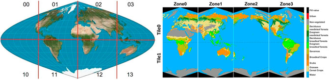
FIGURE 1. (left) Global Sinusoidal projection in v1 MAIAC, and (right) Rotated Sinusoidal projection with global land cover types in v2 MAIAC EPIC algorithm. Also shown are the respective tiling systems.
The v1 MAIAC EPIC used a global Sinusoidal projection (Figure 1, left). This is an equal area projection which is an important property for the land analysis and applications. A serious limitation of this projection is the geographic distortions which grow away from the Greenwich meridian and equator. We introduced a rotated Sinusoidal projection (Figure 1, right) in v2 MAIAC EPIC. It is the same Sinusoidal projection rotated 90° four times to represent an entire landmass as well as the global ocean with significantly reduced distortions. There is a certain overlap between tiles, for instance Alaska can be found at the edge of tile 03 and near center of tile 02. The new projection keeps an equal area property, reduces geographic distortions, and can be easily re-projected to any standard projection without loss of information. It also keeps the same total number of pixels by filling in the significant empty space in the global Sinusoidal projection. For convenience, we offer data users a global mask of pixels with best representation (minimum distortions) to address the problem of overlap.
Cloud Detection
MAIAC EPIC cloud mask algorithm consists of a group of tests that are designed to detect clouds with different spectral/spatial characteristics from the clear-sky conditions. As MAIAC does not require cloud type information, the cloud tests are applied sequentially, and the processing is terminated once cloud is detected.
Brightness Test
The brightness test aims to detect optically thick bright clouds that have a high albedo in the visible spectrum. A pixel is masked as cloud if the measured reflectance (Rm) exceeds the theoretical value at maximal AOD = 6 of the MAIAC look-up table (LUT) at a given view geometry (Rmax) with a certain threshold:
The threshold is 0.1 over bright Sahara region and 0.05 otherwise. The brightness test uses the EPIC blue channel (443 nm), where the surface is generally dark, and the reduction of TOA reflectance by absorbing aerosols (smoke/dust) and the difference in reflectance with non-absorbing clouds is maximal compared to longer wavelengths.
Spatial Variability Test
In general, clouds exhibit a larger spatial variance than aerosol and the ocean surface. The spatial variance test computed using 3 × 3 pixel window has been a standard technique for cloud detection over the ocean at moderate resolution ∼1 km (e.g., Martins et al., 2002). Based on simulated EPIC observations from 1 km MODIS data, we selected the spatial variance threshold of 0.005 which achieves a reasonable balance between cloud filtering and fraction of clear pixels.
Over land surfaces, using a global threshold is problematic due to spatial variability of the land surface reflectance, in particular over bright deserts, in the urban regions and over agricultural areas. Working with gridded data, MAIAC keeps memory of the 3 × 3 standard deviation (σ) for each 10 km grid cell derived in cloud-free and low aerosol conditions. Similar to MAIAC MODIS, σ is computed for the red and blue bands and updated on cloud-free days from observations closest to nadir, when the observation footprint is minimal and spatial variance from surface is maximal. The implementation for EPIC follows test (C.4) in Lyapustin et al. (2018).
High Cloud Test
Detection of optically thin high clouds relies on EPIC measurements in the oxygen A-band. While this signal is low in cloud-free conditions due to absorption by molecular oxygen, presence of high clouds creates a relatively strong signal. Detection of high clouds employs a reflectance ratio measurement of oxygen A-band to the window channel (780 nm) divided by a theoretical reflectance ratio for surface elevation (Z) (Zhou et al., 2020):
where τO2A and τO2A,Z are optical depth values due to O2 absorption from the measured ratio and from the theoretical LUT, respectively, and m = 1/μ0 + 1/μ is an atmospheric airmass factor depending on cosines of solar (μ0), and view (μ) zenith angles. A simple threshold-based approach is then used for high cloud detection: the pixel is considered cloudy if
Similarly to MAIAC MODIS, the above tests only serve for an initial cloud screening. The cloud mask is significantly enhanced following aerosol retrievals by limiting the small-scale spatial variability of AOD, and during the atmospheric correction through comparison of spectral reflectance with the predicted values based on the BRDF model.
Aerosol Retrieval Over Land
Aerosol Models
Following MAIAC MODIS Collection 6 algorithm, we are using eight prescribed regional aerosol models to represent variability of aerosol properties over global land. Geographic distribution and model parameters are provided in Lyapustin et al. (2018, Figure 4 and Table 1).
One known issue in MAIAC C6 was underestimation of AOD for the biomass burning aerosol at high AOD (e.g., Lyapustin et al., 2018; Schutgens et al., 2020; Sogacheva et al., 2020). As a remedy, in MODIS MAIAC C6.1 we adjusted the model parameters at AOD>0.6 based on the regional climatology analysis of the AERONET (Holben et al., 1998; Giles et al., 2019; Sinyuk et al., 2020) record. Similarly, to correct the known low bias of the mineral dust AOD over Western Sahara, we introduced a new corresponding region with the more absorbing dust model. These amendments are used in the v2 MAIAC EPIC and will be described in detail elsewhere.
Aerosol Retrieval Algorithm
MAIAC processing uses the ancillary NCEP ozone and column water vapor information. The over ocean processing also uses the NCEP wind speed.
Retrieval of SRC is a central component of MAIAC: it provides separation of the surface and atmospheric signals in the TOA measurements, and is required for aerosol retrievals. Because EPIC lacks the 2130 nm channel used in MAIAC MODIS, we define SRC as the ratio of the surface reflectance in Blue to Red (SRC = ρL,Blu/ρL,Red) bands. Reflectance ρL,λ is a Lambertian reflectance resulting from the Rayleigh atmospheric correction with low background aerosol. SRC is obtained as a minimum value over the 2-month period of time. Following Lyapustin et al. (2018), we are using two independent lines of update, shifted by 1 month. Thus, the SRC is dynamically updated at least every month or more frequently if a new minimum value is found. SRC is characterized in 4 bins in cosine of the solar zenith angle 1–0.9, 0.9–0.7, 0.7–0.45, and 0.45–0.2. The SRC for the morning and the afternoon observations is separate because of the change in geometry at a near-constant scattering angle, e.g., depending on the part of the orbit, the view zenith angle (VZA) may be higher than the solar zenith angle (SZA) in the morning but symmetrically lower in the afternoon and vice versa.
The AOD is obtained by matching the observed and theoretical TOA reflectance at 443 nm based on the look-up table. The surface reflectance ρB is evaluated from the atmospherically corrected ρL,Red (AOD) at 680nm, ρL,Blu = SRC*ρL,Red. This AOD is derived using the corresponding regional background aerosol models. When derived AOD is high (>0.6) and absorbing smoke or dust is detected, the v2 MAIAC runs a separate inversion of UV-vis observations providing AOD and spectral aerosol absorption (Lyapustin et al., 2021a, this issue).
At high altitudes (over 3.5 km, e.g. Tibetan plateau) where AOD is generally very low and MAIAC AOD retrievals do not have sufficient accuracy, we assume a fixed climatology AODmin = 0.02 for the atmospheric correction.
AERONET AOD Validation
To assess accuracy of AOD retrieval, we conducted AERONET validation for 2015–2020 using level 2.0 AERONET version 3 data (Giles et al., 2019). The comparison uses EPIC AOD at 443 nm averaged over the 5 × 5 pixels window (50 km) with AERONET data selected within 30 min from the satellite observation. The EPIC data were filtered according to the Sun and view zenith angles less than ∼63° and at least 50% coverage in the spatial window.
The validation results are presented in Figure 2. The site-level global statistics shows the correlation coefficient (R), root mean square error (RMSE) and the mean bias error (MBE, MAIAC–AERONET). MAIAC shows a good retrieval accuracy, with R ≥ 0.7–0.8 and low RMSE and MBE, over vegetated parts of the world including North and South America, north-central Eurasia and Oceania. AOD is generally overestimated over bright surfaces such as western United States and Australia. Such bias is typical for aerosol products based on a single-view satellite measurement, and it is exacerbated for EPIC due to unfavorable view geometry near the backscattering direction. The underestimation of AOD is obvious in regions of strong biomass burning, including central Africa, Indo-Gangetic plain and south Asia. Similar to the bias, the RMSE is generally low globally with the exception of the major dust and biomass burning aerosol source regions which also have a much higher annual average AOD. The correlation is generally high in regions with higher magnitude and variability of AOD. On the contrary, the low correlation is observed over regions with low aerosol loading and low natural variability, such as Australia or south of the South American continent.
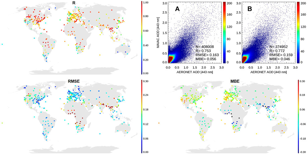
FIGURE 2. Global AERONET validation of MAIAC EPIC AOD at 443 nm. The geographic distribution of the site-level results is displayed for the regression coefficient (R), root mean square error (RMSE) and the mean bias error (MBE). The two scatterplots show the summary validation using all AERONET sites (A) and its subset with 12 bright sites (see Aeronet AOD Validation) excluded.
The two scatterplots on the right summarize the global validation analysis. The left one 1) shows all AERONET sites. On the right scatterplot (b), we excluded 11 bright surface sites over the Western United States (Bakersfield; Goldstone; KeyBiscayne; Neon_ONAQ; Railroad Valley; Sandila_NM_PSEL; TableMountain_CA; Tucson; UACJ_UNAM_ORS; White_Sands_HELSTF; Yuma) and one site over Australia (Birdsville). These sites are located in arid regions with low AOD and low AOD variability where MAIAC EPIC overestimates AOD and shows low R-values. Due to low cloudiness, these sites also contribute a disproportionate ∼9% of the total matching points. Considering the right scatterplot as a baseline, MAIAC shows an overall correlation of 0.77 with RMSE ∼ 0.159 and a mean bias of 0.046. Over 66.72% of MAIAC EPIC AOD agree with AERONET within the expected error (EE) of ±(0.1 + 0.1AOD). The v2 shows an improvement over v1 which had a global statistics of R = 0.69, RMSE = 0.17, MBE = 0.03 (unpublished).
Atmospheric Correction Over Land
Following cloud detection and aerosol retrieval, the atmospheric correction (AC) algorithm derives spectral surface reflectance and updates the Ross-Thick Li-Sparse (RTLS, Lucht et al., 2000) BRDF model parameters,
Here, volumetric (fV) and geometric-optics (fG) kernels are functions of the view geometry, and pixel-specific weights (kL, kV,kG) describe different BRDF shapes. To account for the surface reflectance increase in the backscattering view geometry of EPIC, the volumetric kernel is multiplied by the hot-spot factor as suggested by Maignan et al. (2004) based on POLDER observations.
Atmospheric Correction: MAIAC Scaling Approach
The v1 MAIAC EPIC algorithm used a Lambertian model for the atmospheric correction, where the surface reflectance is derived from the following approximation to the TOA reflectance:
Eq. 4 only requires the knowledge of atmospheric (path) reflectance (RA), upward (Tu) and downward (Td) atmospheric transmittance as functions of the cosines of Sun (μ0) and view (μ) zenith angles and relative azimuth (φ), and spherical albedo of atmosphere (s). In the EPIC view angles near the hotspot where surface is brighter than in the other directions, the Lambertian approximation underestimates the surface reflectance (e.g., Wang et al., 2010). An analysis of Lambertian biases was recently given by Lyapustin et al. (2021b) based on a comparison between the two MODIS surface reflectance products, the standard surface reflectance (SR) MOD09 based on Lambertian assumption, and the bidirectional reflectance factors (BRF) of algorithm MAIAC (MCD19A1).
The MAIAC atmospheric correction uses a rigorous expression for the TOA reflectance. Taking advantage of linearity of the RTLS function, it represents the TOA reflectance explicitly using weights of the RTLS model:
Here, F-functions are integrals of the atmospheric path radiance incident on surface and atmospheric Green’s function (Lyapustin and Knyazikhin, 2001) with respective kernels of the RTLS model. Rnl is a weakly non-linear function of the surface reflectance, describing multiple light scattering between the surface and the atmosphere. The F-functions and Rnl are computed analytically using eight primary functions which are stored in the MAIAC LUT (e.g., Lyapustin et al., 2011a). For the purpose of atmospheric correction, let us re-write Equation 5 as follows:
where RSurf is a surface-reflected term combining the last four terms of Eq. 5, and c ≡ cλ is a spectrally dependent scaling factor. The RSurf is computed using the BRDF model parameters stored in MAIAC memory for each grid cell (e.g., 1 km for MODIS and 10 km for EPIC). Then, the BRF is given by a scaled value:
where RTLSλ is the BRDF model value for a given geometry. Because RSurf is a nonlinear function of the surface reflectance, solving eqs. (6) and (7) takes 2 iterations (see Lyapustin et al., 2018, p. 5753).
Implementing rigorous atmospheric correction given by Eqs. (6) and (7). requires knowledge of the entire BRDF shape to correctly represent surface reflection of the direct Sun beam and of the diffuse (sky) light. In v2 MAIAC EPIC, we used the global Collection 6 MAIAC MODIS 1 km BRDF product MCD19A3 to develop an ancillary BRDF dataset for the EPIC 10-km grid from the closest MODIS channels. The AC based on Eqs. (6) and (7). uses scaling approach and only requires knowledge of the relative BRDF shape rather than the absolute reflectance. For this reason, the wavelength difference between the EPIC and MODIS channels is not important as long as the land surface reflectance among the paired channels, and thus the BRDF shape, remain similar. The ancillary 10 km BRDF for EPIC was created for every month starting in 2015. Figure 3 illustrates the global RGB BRDF for nadir view and Sun at 45° for January and July of 2016.
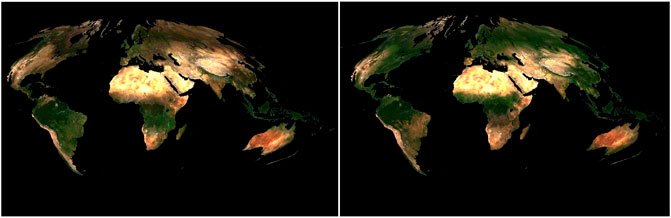
FIGURE 3. The monthly average RGB surface BRDF for February (left) and July (right) of 2016 from MAIAC MODIS MCD19A3 product.
Figure 4 gives an example of atmospheric correction based on scaling (S) in the Blue and Red bands in columns 3 and 5, respectively. The result is shown as an excess of anisotropic over the Lambertian reflectance (BRF-ρL)/ρL (%). In agreement with theory, the difference is lowest when the Sun is near zenith, and it grows with the atmospheric airmass factor. It also increases with the total atmospheric optical thickness from NIR to Blue, for instance from ∼3% at 780nm, ∼10% at 680nm to 60–80% at 443 nm at high Sun/view zenith angles (μ0,μ ∼ 0.2). While this pattern agrees with theoretical expectations in general, the strong increase of BRF at high zenith angles, in particular at 443nm, does not seem realistic.
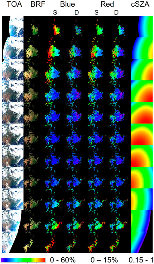
FIGURE 4. Analysis of different schemes of atmospheric correction of EPIC over North America on June 13, 2020. The first and second columns show the EPIC’s TOA and atmospherically corrected RGB BRF images. Columns 3–6 show the relative difference between anisotropic BRF and Lambert (ρL) reflectance (BRF-ρL/ρL)×100% in the Blue and Red bands, where BRF was computed using the scaling (S) and the “direct term” (D) methods. The last column displays the cosine of the solar zenith angle.
Atmospheric Correction: Separation of the Direct and Diffuse Reflectance
The scaling approach Eqs. (6) and (7) assumes that the BRDF model gives a good description of the surface reflectance at the angles of satellite observations. In this case, direct and diffuse surface-reflected signals at the TOA can be scaled using the same multiplier c. This approach works for MAIAC MODIS where the BRDF represents the view geometry sampled by MODIS. The ancillary MODIS BRDF was derived for the range of SZA observed near the local noon around 10:30 am (Terra) and 1:30 pm (Aqua) equatorial crossing time. Thus, it can be considered representative of the EPIC’s view geometry within about ±2 h of the local noon. Outside of that range, at higher SZA both earlier in the morning and later in the afternoon, the MODIS BRDF can still be used to compute the reflection of the diffuse sky irradiance assuming BRDF reciprocity, at least for the range of SZA agreeing with the VZA range of MODIS, ∼0–62° accounting for the Earth’s curvature. However, it cannot represent correctly the direct TOA reflectance ρ(μ0,μ,φ)exp(−mτ), where τ is an atmospheric optical depth, as MODIS does not make measurements at higher SZAs near the hotspot.
In this case, we can single out the direct reflectance in Eq. 6:
where the diffuse component of the surface-reflected signal at TOA is:
Above, ρ is the true surface BRF, and RDif and RTLS are computed with the ancillary MODIS BRDF. The gλ is the spectral adjustment factor designed to account for the surface reflectance difference from the spectral shift between the paired EPIC - MODIS channels, e.g., for the Blue (443/465.5 nm), Green (555/553.5 nm), Red (680/644.9 nm) and NIR (779.5/855.6 nm) EPIC/MODIS center wavelengths, respectively. For each 10 km pixel, we compute the spectral adjustment factor gλ using scaling atmospheric correction (Eqs. (6) and (7) near the local noon (within Δμ0 of ±0.1) where MODIS BRDF should be valid for both direct and diffuse terms, as we discussed above. In this case, gλ is equivalent to the scaling factor cλ. The gλ is computed daily for each cloud-free 10 km grid cell at low AOD and is stored in MAIAC memory until updated with the next retrieval. Such approach allows us to evaluate the diffuse reflected term using the ancillary MAIAC MODIS BRDF, and compute BRF (ρ) from the direct reflected term in Eq. 8.
The described “direct term” (D) algorithm is more generic than the scaling approach. The resulting BRFD (columns 4 and 6 of Figure 3 for the Blue and Red bands, respectively) can be compared to the scaling BRFS in Figure 4. BRFD shows a more constrained increase over the Lambertian reflectance up to SZA∼70° which grows only to ∼35% in the Blue band instead of ∼60–80% for the scaling approach. Importantly, the anisotropic enhancement (of the Lambertian reflectance) remains nearly constant in the range of SZA∼0–60°, though the uncertainty Δρ increases at high EPIC SZA/VZA. The uncertainty is twofold: it is related to both the aerosol retrieval uncertainty (Δτ) and to the uncertainty in the diffuse signal RDif introduced by the MODIS BRDF (ΔRTLS) which was defined for a relatively narrow range of SZA values of MODIS Terra and Aqua at a fixed overpass time, and the limited range of VZA≤62°. Moreover, while working well in the range of SZA/VZA∼60°, the RTLS BRDF model has the problem of unconstrained growth of both geometric-optics and volumetric kernels at higher SZA/VZA, proportionally to a combination of terms 1/μ0, 1/μ (e.g., Gao et al., 2000). Finally, a significant uncertainty is related to the increase of the EPIC’s footprint with VZA faster than 1/μ while the ancillary BRDF generated from 1 km MODIS still closely represents the 10 km grid box. For these reasons, the atmospheric correction problem (Eqs. (6) and (7) at high zenith angles becomes ill-posed and poorly constrained, with an exponential propagation of uncertainties:
Atmospheric Correction for EPIC
The above analysis showed limitations of both scaling and the “direct term” atmospheric correction methods, in particular at high SZA/VZA. The main limitations stem from the limited angular sampling of EPIC prohibiting deriving the self-consistent BRDF model in the full hemisphere of angles of incidence and reflection, and from the growing uncertainties of the ancillary MODIS BRDF model at high SZA/VZA in application to EPIC. Both Lambertian and scaling algorithms reproduce well the spatial pattern and the RGB color of the EPIC TOA images while, respectively, underestimating and overestimating the true BRF, especially at high zenith angles. The “direct term” algorithm shows rapidly growing uncertainties at high zenith angles. As it depends on the absolute ancillary BRDF model, this approach is also prone to spatial and spectral distortions in the resulting RGB BRF images. At the same time, this algorithm provides a realistic more constrained BRF increase over the Lambertian value, and a near-constant u = BRF/ρL ratio in the wide range of zenith angles up to ∼50–60°. This ratio fully agrees with the BRF/ρL ratio of the scaling method evaluated for the observations near the local noon.
Given these findings, the MAIAC EPIC v2 AC approach in RGB and NIR bands is implemented as follows:
- Compute the Lambertian reflectance (ρL,λ) from Eq. 4;
- Compute BRF as ρ(μ0,μ,φ) = ρL,λuλ;
- The anisotropic conversion factor uλ is derived from “scaling” BRFS, uλ = BRFS/ρL,λ, computed near the local noon where the scaling approach is valid. It is updated daily from the cloud-free observations near the local noon (within Δμ0 of ±0.1) and is stored in MAIAC′ memory for each 10 km grid cell.
The anisotropic conversion factor near the local noon gives the increase over the Lambertian reflectance from 1–2% at 780 nm to 8–15% at 443 nm. The uncertainty of the reported BRF is low for the EPIC observations near the local noon, and it is expected to significantly increase at zenith angles above ∼60°. The selected empirical AC approach is fast and does not create spectral distortions, but it probably underestimates BRF at higher zenith angles. In near future, we plan to further explore both “scaling” and the “direct term” AC algorithms using BRDF model from the geostationary satellites which provide the full range of the solar zenith angle variations.
The MAIAC v2 algorithm reports both ρL and BRF reflectance values in the RGB and NIR channels. In the UV, where uncertainties are the largest, only the Lambertian reflectance is reported.
Figure 5 gives an example of atmospheric correction for the 1-month period of June 2–July 2, 2020, for a single 10 km bright surface grid cell in Arizona, United States. The derived surface reflectance displays a well-reproducible daily pattern in the visible–near infrared with surface reflectance increasing with SZA. The strongest growth is observed in the NIR in agreement with (Marshak, 2021). The pattern becomes less certain at UV wavelengths: the SR points tend to cluster within about ±0.01 of the mid-day value with occasional high and low outliers at both 388 and 340 nm wavelengths. On average, the AC produces a correct pattern with ρ340<ρ388 at μ,μ0 above ≈0.6 (53°), and unstable result at higher SZA/VZA. This result is rather systematic and holds over both bright and dark vegetated surfaces. As the uncertainty in the UV SR rapidly grows with the airmass factor, the most accurate SR values at 340 and 388 nm are reported near the local noon.
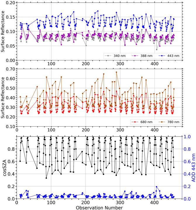
FIGURE 5. The time series of surface reflectance in EPIC’s UV-vis-NIR bands over the bright pixel in Arizona, United States, in June–early July of 2020. The bottom plot shows cosine of solar zenith angle and retrieved AOD at 443 nm. The x-axis counts consecutive EPIC observations from June 2 through July 2 of 2020.
Retrieving BRDF Model Parameters
Following computation of BRF, MAIAC proceeds with calculation of the RTLS parameters (K-coefficients) using the multi-angle dataset accumulated in the MAIAC Queue memory for each grid cell (up to 40 observations). This retrieval is performed for the four visible and near-IR bands only. After inversion, the new BRDF goes through several tests verifying “correctness” of its shape, and its consistency with the previous solution (Lyapustin et al., 2012). Figure 6 shows the daily BRF pattern (dots connected by solid lines) in the Blue-NIR EPIC bands for the pixel displayed in Figure 5 on two different days in June of 2020. The best-fit BRDF model is shown by the dashed lines. While the BRDF model error can reach several absolute percent of reflectance at high zenith angles, the typical rmse of the fit is low, within ∼0.001–0.002.
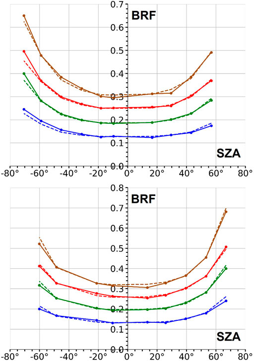
FIGURE 6. An example of the retrieved BRF (dots connected by solid lines) and the best-fit BRDF model (dashed lines) for the bright surface pixel displayed in Figure 5. The BRF and BRDF are shown for 2 different days in June of 2020 in RGB bands (in respective color) and in the NIR (in brown). The SZA is positive in the morning, and negative in the afternoon.
It should be mentioned that the derived BRDF model describes only the range of the EPIC observations within 4–12° from the backscattering direction, and is not representative of the general BRDF shape. A failure of the DSCOVR gyroscopes in late June of 2019 led to EPIC being placed in a safehold mode till March of 2020. This period was required to find the engineering solution for the satellite navigation using startrackers and update the geolocation algorithm. After resuming operation, the DSCOVR orbit became less constrained and allows the range of angles ∼2–12° from the exact backscattering since March 2020.
Concluding Remarks
This paper described the version 2 MAIAC land algorithm developed for processing of the DSCOVR EPIC data. The full MAIAC processing includes cloud detection, aerosol retrieval and atmospheric correction over both land and ocean.
Following MODIS, the standard MAIAC aerosol retrieval uses the regional background aerosol models to derive AOD. A global validation of AOD using AERONET for the period of 2015–2020 shows the overall good performance with R = 0.77, RMSE = 0.159, and MBE = 0.046. The v2 shows an improvement over v1 MAIAC (R = 0.67, RMSE = 0.17) and compares favorably to MAIAC MODIS Collection 6 (R = 0.84, RMSE = 0.12, MBE = 0.01 (Lyapustin et al., 2018)) despite coarse spatial resolution and the backscattering view geometry. The positive bias of v2 MAIAC EPIC mostly comes from the retrievals over bright surfaces.
In cloud-free conditions, the retrieved AOD along with the ancillary NCEP ozone and water vapor information is used for the atmospheric correction of EPIC. MAIAC v2 reports AC results using both Lambert and anisotropic SR models. The Lambert model systematically underestimates SR in the EPIC’s view geometry. The anisotropic atmospheric correction uses the ancillary monthly BRDF database based on MAIAC MODIS C6 RTLS BRDF. The uncertainties of anisotropic AC come from very different view geometries of MODIS and EPIC which overlap only for EPIC observations near the local noon. For this reason, the standard MAIAC scaling AC algorithm works only for the range of EPIC observations near the local noon. On the other hand, BRF retrieval from the direct surface-reflected term show a stable (BRF-ρL)/ρL ratio in the wide range of EPIC’s SZA. This led us to adapt a simple AC approach in the vis-NIR bands by upscaling the Lambertian SR, where the scale factor is computed from the EPIC observations near the local noon. At low to moderate AOD, the typical (BRF-ρL)/ρL ratio near the local noon is ∼1–2% in the NIR, and ∼8–15% in the Blue EPIC bands.
Due to higher uncertainties, the AC in the UV uses the Lambertian model. It produces rather consistent results with uncertainty of about ±0.01 or less for Sun/view zenith angles less than ∼53°, with most reliable retrievals near the local noon. At higher zenith angles, the UV SR may become unstable.
Over land, the MAIAC EPIC product suite includes the background model AOD at 443 and 550 nm, Lambert surface reflectance at 340, 388, 443, 551, 680 and 780 nm, and BRF and the BRDF model parameters for the RTLS model at 443, 551, 680 and 780 nm. It is important to note that the BRDF model is only relevant for the near hot-spot cone of the scattering angles observed by EPIC, although it covers the full range of variation in the Sun and view zenith angles. The reported spectral BRF is used as an input for Level 2 Vegetation Earth System Data Record (VESDR) (Yang et al., 2017; NASA/LARC/SD/ASDC-VESDR, 2021).
Over water, MAIAC data products include AOD, fine mode fraction (FMF) and Angstrom exponent, and “ocean color” (water-leaving reflectance) at 340, 388, 443, 551, 680 and 780 nm.
For detected absorbing smoke and dust aerosols, the v2 MAIAC retrieves AOD and spectral imaginary refractive index characterizing aerosol absorption from EPIC’s UV-vis measurements. This capability was described in Lyapustin et al. (2021a). In this case, the v2 MAIAC reports AOD, single scattering albedo (SSA) at 443 nm, spectral absorption exponent (SAE) and imaginary refractive index at 680nm, and the goodness of fit for two effective heights of aerosol layer at 1 and 4 km.
The daily rate of global MAIAC retrievals ranges on average from 15 to 27%, reaching maximum during the boreal summer. This number is a proxy of the global cloud- and snow-free fraction of the Earth. The MAIAC product is distributed as compressed HDF5 files. The lossless compression gives approximately a 10-fold reduction of the file size, resulting in an average size of ∼30 Mb.
The re-processing of version 3 EPIC L1B dataset for 2015–June 2021 with v2 MAIAC algorithm has been completed. The MAIAC EPIC products will soon be available for downloading from the Atmospheric Science Data Center (ASDC) at NASA Langley Research Center.
Data Availability Statement
The datasets presented in this study can be found in online repositories. The names of the repository/repositories and accession numbers can be found below: NASA/LARC/SD/ASDC, 2018. DSCOVR EPIC L2 Multi-Angle Implementation of Atmospheric Correction (MAIAC) Atmospheric Correction data product. Available at: https://doi.org/10.5067/EPIC/DSCOVR/L2_MAIAC.001.
Author Contributions
AL, DH, YW, and SK adapted MAIAC algorithm for EPIC; YW performed re-processing of EPIC data; SG and MC performed aerosol validation analysis; KB developed the geolocation algorithm; AL and DH wrote the initial draft of paper. All contributed to preparing the final version of the manuscript.
Funding
This work was funded by the NASA DSCOVR program (manager R. Eckman). We are grateful to the AERONET team for providing validation data and to the NASA Center for Climate Simulations used for the EPIC data processing.
Conflict of Interest
At the time of this work, author DH was employed by the Science Systems and Applications Inc., Lanham, MD, United States (SSAI), and currently he is with the IEX Group, New York, NY.
The remaining authors declare that the research was conducted in the absence of any commercial or financial relationships that could be construed as a potential conflict of interest.
Publisher’s Note
All claims expressed in this article are solely those of the authors and do not necessarily represent those of their affiliated organizations, or those of the publisher, the editors and the reviewers. Any product that may be evaluated in this article, or claim that may be made by its manufacturer, is not guaranteed or endorsed by the publisher.
References
Blank, K., Huang, L.-K., Herman, J., and Marshak, A. (2021). EPIC Geolocation; Strategies to Reduce Uncertainty. Front. Remote Sens. (submitted May 26, 2021).
Cede, A., Huang, L. K., McCauley, G., Herman, J., Blank, K., Kowalewski, M., et al. (2021). Raw EPIC data calibration. Front. Remote Sens. 2. doi:10.3389/frsen.2021.702275
Doelling, D., Haney, C., Bhatt, R., Scarino, B., and Gopalan, A. (2019). The Inter-Calibration Of The Dscovr Epic Imager With Aqua-Modis And Npp-Viirs. Remote Sensing 11, 1609. doi:10.3390/rs11131609
Gao, F., Li, X., Strahler, A., and Schaaf, C. (2000). Evaluation of the Li Transit Kernel for BRDF Modeling. Remote Sensing Rev. 19 (1-4), 205–224. doi:10.1080/02757250009532419
Geogdzhayev, I. V., Marshak, A., and Alexandrov, M. (2021). Calibration Of The Dscovr Epic Visible And Nir Channels Using Multiple Leo Radiometers. Front. Remote Sens. 2, 671933. doi:10.3389/frsen.2021.671933
Geogdzhayev, I. V., and Marshak, A. (2018). Calibration Of The Dscovr Epic Visible And Nir Channels Using Modis Terra And Aqua Data And Epic Lunar Observations. Atmos. Meas. Tech. 11, 359–368. doi:10.5194/amt-11-359-2018
Gerstl, S. A. W. (1999). Building a Global Hotspot Ecology with Triana Data. Remote Sens. Earth Science, Ocean, Sea Ice Appl. 3868, 184–194. doi:10.1117/12.373094
Giles, D. M., Sinyuk, A., Sorokin, M. G., Schafer, J. S., Smirnov, A., Slutsker, I., et al. (2019). Advancements in the Aerosol Robotic Network (AERONET) Version 3 Database - Automated Near-Real-Time Quality Control Algorithm with Improved Cloud Screening for Sun Photometer Aerosol Optical Depth (AOD) Measurements. Atmos. Meas. Tech. 12, 169–209. doi:10.5194/amt-12-169-2019
Herman, J., Huang, L., McPeters, R., Ziemke, J., Cede, A., and Blank, K. (2018). Synoptic Ozone, Cloud Reflectivity, and Erythemal Irradiance from Sunrise to sunset for the Whole Earth as Viewed by the DSCOVR Spacecraft from the Earth-Sun Lagrange 1 Orbitflectivity, and Erythemal Irradiance from Sunrise to sunset for the Whole Earth as Viewed by the DSCOVR Spacecraft from the Earth–Sun Lagrange 1 Orbit. Atmos. Meas. Tech. 11, 177–194. doi:10.5194/amt11-177-201810.5194/amt-11-177-2018
Holben, B. N., Eck, T. F., Slutsker, I., Tanré, D., Buis, J. P., Setzer, A., et al. (1998). AERONET-A Federated Instrument Network and Data Archive for Aerosol Characterization. Remote Sensing Environ. 66, 1–16. doi:10.1016/s0034-4257(98)00031-5
Lucht, W., Schaaf, C. B., and Strahler, A. H. (2000). An Algorithm for the Retrieval of Albedo from Space Using Semiempirical BRDF Models. IEEE Trans. Geosci. Remote Sensing 38, 977–998. doi:10.1109/36.841980
Lyapustin, A., Go, S., Korkin, S., Wang, Y., Torres, O., Jethva, H., et al. (2021a). Retrievals of Aerosol Optical Depth and Spectral Absorption from DSCOVR EPIC. Front. Remote Sens. 2, 645794. doi:10.3389/frsen.2021.645794
Lyapustin, A. I., Wang, Y., Laszlo, I., Hilker, T., G.Hall, F., Sellers, P. J., et al. (2012). Multi-angle Implementation of Atmospheric Correction for MODIS (MAIAC): 3. Atmospheric Correction. Remote Sensing Environ. 127, 385–393. doi:10.1016/j.rse.2012.09.002
Lyapustin, A., and Knyazikhin, Y. (2001). Green's Function Method for the Radiative Transfer Problem I Homogeneous Non-lambertian Surface. Appl. Opt. 40, 3495–3501. doi:10.1364/AO.40.003495
Lyapustin, A., Martonchik, J., Wang, Y., Laszlo, I., and Korkin, S. (2011a). Multiangle Implementation of Atmospheric Correction (MAIAC): 1. Radiative Transfer Basis and Look-Up Tables. J. Geophys. Res. 116, D03210. doi:10.1029/2010JD014985
Lyapustin, A., Wang, Y., Korkin, S., and Huang, D. (2018). MODIS Collection 6 MAIAC Algorithm. Atmos. Meas. Tech. 11, 5741–5765. doi:10.5194/amt-11-5741-2018
Lyapustin, A., Wang, Y., Laszlo, I., Kahn, R., Korkin, S., Remer, L., et al. (2011b). Multiangle Implementation of Atmospheric Correction (MAIAC): 2. Aerosol Algorithm. J. Geophys. Res. 116, D03211. doi:10.1029/2010JD014986
Lyapustin, A., Zhao, F., and Wang, Y. (2021b). A Comparison of Multi-Angle Implementation of Atmospheric Correction (MAIAC) and MOD09 Daily Surface Reflectance Products from MODIS. Front. Remote Sens. (in review).
Maignan, F., Bréon, F.-M., and Lacaze, R. (2004). Bidirectional Reflectance of Earth Targets: Evaluation of Analytical Models Using a Large Set of Spaceborne Measurements with Emphasis on the Hot Spot. Remote Sensing Environ. 90 (2), 210–220. doi:10.1016/j.rse.2003.12.006
Marshak, A. (2021). Alfonso Delgado-Bonal and Yuri Knyazikhin, Effect of Scattering Angle on Earth Reflectance. Front. Remote Sens. in review.
Marshak, A., Herman, J., Adam, S., Karin, B., Carn, S., Cede, A., et al. (2018). Earth Observations From Dscovr Epic Instrument. Bull. Amer. Meteorol. Soc. 99 (9), 1829–1850. doi:10.1175/BAMS-D-17-0223.1
Martins, J. V., Tanré, D., Remer, L., Kaufman, Y., Mattoo, S., and Levy, R. (2002). MODIS Cloud Screening for Remote Sensing of Aerosols over Oceans Using Spatial Variability. Geophys. Res. Lett. 29 (12), 1619. doi:10.1029/2001GL013252
NASA/LARC/SD/ASDC-VESDR (2021). Dscovr Epic Level 2 Vegetation Earth System Data Record (Vesdr), Version 2. In: NASA Langley Atmospheric Science Data Center DAAC, doi:10.5067/EPIC/DSCOVR/L2_VESDR.002
Schutgens, N., Sayer, A. M., Heckel, A., Hsu, C., Jethva, H., de Leeuw, G., et al. (2020). An AeroCom-AeroSat Study: Intercomparison of Satellite AOD Datasets for Aerosol Model Evaluation. Atmos. Chem. Phys. 20, 12431–12457. doi:10.5194/acp-20-12431-2020
Sinyuk, A., Holben, B. N., Eck, T. F., Giles, D. M., Slutsker, I., Korkin, S., et al. (2020). The AERONET Version 3 Aerosol Retrieval Algorithm, Associated Uncertainties and Comparisons to Version 2. Atmos. Meas. Tech. 13, 3375–3411. doi:10.5194/amt-13-3375-2020
Sogacheva, L., Popp, T., Sayer, A. M., Dubovik, O., Garay, M. J., Heckel, A., et al. (2020). Merging Regional and Global Aerosol Optical Depth Records from Major Available Satellite Products. Atmos. Chem. Phys. 20, 2031–2056. doi:10.5194/acp-20-2031-2020
Wang, Y., Lyapustin, A. I., Privette, J. L., Cook, R. B., SanthanaVannan, S. K., Vermote, E. F., et al. (2010). Assessment of Biases in MODIS Surface Reflectance Due to Lambertian Approximation. Remote Sensing Environ. 114, 2791–2801. doi:10.1016/j.rse.2010.06.013
Yang, B., Knyazikhin, Y., Mõttus, M., Rautiainen, M., Stenberg, P., Yan, L., et al. (2017). Estimation Of Leaf Area Index And Its Sunlit Portion From Dscovr Epic Data: Theoretical Basis. Remote Sensing Environ. 198, 69–84. doi:10.1016/j.rse.2017.05.033
Yang, Y., Meyer, K., Wind, G., Zhou, Y., Marshak, A., Platnick, S., et al. (2019). Cloud Products from the Earth Polychromatic Imaging Camera (EPIC): Algorithms and Initial Evaluation. Atmos. Meas. Tech. 12, 2019–2031. doi:10.5194/amt-12-2019-2019
Keywords: aerosol, surface reflectance, bidirectional reflectance distribution function, multi-angle implementation of atmospheric correction, atmospheric correction, EPIC
Citation: Lyapustin A, Wang Y, Go S, Choi M, Korkin S, Huang D, Knyazikhin Y, Blank K and Marshak A (2021) Atmospheric Correction of DSCOVR EPIC: Version 2 MAIAC Algorithm. Front. Remote Sens. 2:748362. doi: 10.3389/frsen.2021.748362
Received: 27 July 2021; Accepted: 02 September 2021;
Published: 20 September 2021.
Edited by:
Feng Xu, University of Oklahoma, United StatesReviewed by:
Bing Lin, National Aeronautics and Space Administration, United StatesShaohua Zhao, Ministry of Ecology and Environment Center for Satellite Application on Ecology and Environment, China
Copyright © 2021 Lyapustin, Wang, Go, Choi, Korkin, Huang, Knyazikhin, Blank and Marshak. This is an open-access article distributed under the terms of the Creative Commons Attribution License (CC BY). The use, distribution or reproduction in other forums is permitted, provided the original author(s) and the copyright owner(s) are credited and that the original publication in this journal is cited, in accordance with accepted academic practice. No use, distribution or reproduction is permitted which does not comply with these terms.
*Correspondence: A. Lyapustin, QWxleGVpLkkuTHlhcHVzdGluQG5hc2EuZ292