Global Daytime Mean Shortwave Flux Consistency Under Varying EPIC Viewing Geometries

One of the most crucial tasks of measuring top-of-atmosphere (TOA) radiative flux is to understand the relationships between radiances and fluxes, particularly for the reflected shortwave (SW) fluxes. The radiance-to-flux conversion is accomplished by constructing angular distribution models (ADMs). This conversion depends on solar-viewing geometries as well as the scene types within the field of view. To date, the most comprehensive observation-based ADMs are developed using the Clouds and the Earth’s Radiant Energy System (CERES) observations. These ADMs are used to derive TOA SW fluxes from CERES and other Earth radiation budget instruments which observe the Earth mostly from side-scattering angles. The Earth Polychromatic Imaging Camera (EPIC) onboard Deep Space Climate Observatory observes the Earth at the Lagrange-1 point in the near-backscattering directions and offers a testbed for the CERES ADMs. As the EPIC relative azimuth angles change from 168^◦ to 178^◦, the global daytime mean SW radiances can increase by as much as 10% though no notable cloud changes are observed. The global daytime mean SW fluxes derived after considering the radiance anisotropies at relative azimuth angles of 168^◦ and 178^◦ show much smaller differences (<1%), indicating increases in EPIC SW radiances are due mostly to changes in viewing geometries. Furthermore, annual global daytime mean SW fluxes from EPIC agree with the CERES equivalents to within 0.5 Wm⁻² with root-mean-square errors less than 3.0 Wm⁻². Consistency between SW fluxes from EPIC and CERES inverted from very different viewing geometries indicates that the CERES ADMs accurately quantify the radiance anisotropy and can be used for flux inversion from different viewing perspectives.

1 Introduction

The Deep Space Climate Observatory (DSCOVR) was launched on Feb. 11, 2015 and is the first Earth-observing satellite at the Lagrange-1 (L1) point, about 1.6 million kilometers from Earth. DSCOVR is in an elliptical Lissajous orbit around the L1 point and is not positioned exactly on the Earth-Sun line; therefore, only about 92–97% of the sunlit Earth is visible to DSCOVR (Su et al., 2018). Onboard DSCOVR, the National Institute of Standards and Technology Advanced Radiometer (NISTAR) provides continuous full disc global broadband irradiance measurements over most of the sunlit side of the Earth at near-backscattering relative azimuth angles (Figure 1). DSCOVR also carries the Earth Polychromatic Imaging Camera (EPIC) which provides 2048 by 2048 pixel imagery 10 to 22 times per day in 10 spectral bands from 317 to 780 nm. DSCOVR’s elliptical Lissajous orbit is a quasi-periodic orbit and its distance and viewing geometries change from day to day. Figure 2 shows the relative azimuth angles between DSCOVR and the solar plane from 2017 to 2020. From January 2017 to June 2019, the relative azimuth angles show small month-to-month variations and the maximum value does not exceed 175^◦. However, the relative azimuth angles of 2020 show large month-to-month changes (about twice the amplitude of previous years), with the maximum relative azimuth angle exceeding 178^◦ in December.

FIGURE 1

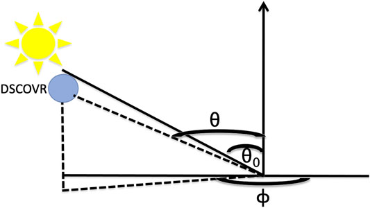
FIGURE 1. DSCOVR viewing geometry, θ₀ is the solar zenith angle, θ is the DSCOVR viewing zenith angle, and ϕ is the relative azimuth angle between DSCOVR and the solar plane.

FIGURE 2

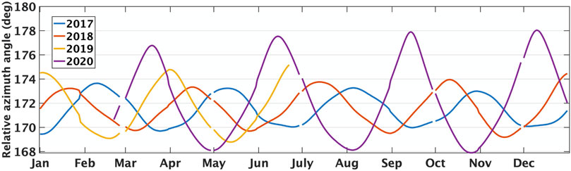
FIGURE 2. Year-to-year variation of the relative azimuth angle for DSCOVR.

Su et al. (2018) developed a methodology to derive global daytime shortwave (SW) flux from EPIC spectral measurements. While EPIC does not measure the entire sunlit side of Earth, we refer to EPIC measurements as “global’ daytime for simplicity. Their approach includes three steps: 1) derive broadband SW radiances from the EPIC narrowband measurements using pre-determined narrowband-to-broadband regression relationships and calculate the global daytime mean radiances ($\overline{I_{sw}}$); 2) derive global daytime mean anisotropy factors ($\overline{R_{sw}}$) using angular distribution models (ADMs, Su et al., 2015a) developed by the Clouds and the Earth’s Radiant Energy System (CERES) project, and using cloud properties in the EPIC cloud composite product (Khlopenkov et al., 2017) for scene identification; 3) derive global daytime mean SW flux: $\overline{F_{sw}}=\pi \overline{I_{sw}}/\overline{R_{sw}}$. These EPIC-based $\overline{F_{sw}}$ agree with the CERES fluxes within the EPIC view to within ±2%, well within the calibration and algorithm uncertainties of each instrument. This is the first time that CERES ADMs have been applied to the near-backscattering direction to derive flux and the good agreement indicates that CERES ADMs accurately account for the Earth’s anisotropy in the near-backscattering direction.

Changes in the EPIC relative azimuth angles in 2020 offer another opportunity to examine whether CERES ADMs can capture the changes in radiance anisotropy as the relative azimuth angles moved from 170^° to 178^°. Anisotropies at these near-backscattering angles are rarely used to invert fluxes for CERES cross track observations. Theoretically, radiative fluxes inverted from different viewing geometries at a given solar zenith angle should be identical. Thus, good agreement between global daytime mean fluxes from EPIC and CERES that are derived using observations from near-backscattering directions and side-scattering directions can be used as an indication of the validity of the ADMs, similar to the consistency tests that have been done to validate the CERES ADMs (Su et al., 2015b). This paper will examine how $\overline{I_{sw}}$ and $\overline{R_{sw}}$ vary with relative azimuth angles and compare $\overline{F_{sw}}$ from EPIC derived at different backscattering directions with CERES counterparts to investigate if CERES ADMs capture the radiance anisotropy changes at different backscattering angles. Section 2 briefly describes the method used to derive EPIC-based broadband SW radiance and compares the radiances from EPIC under different relative azimuth angles. To convert radiances to fluxes, we rely on CERES ADMs which are functions of scene types defined using many variables (i.e., surface type, cloud fraction, cloud optical depth, cloud phase, etc). Section 3 describes the EPIC cloud composite product developed from cloud retrievals using imagers on low-Earth orbit and geostationary satellites. The EPIC cloud composite is used to provide scene identification for anisotropy characterization. Section 4 provides an overview of the CERES ADMs. EPIC-based SW fluxes and comparisons with CERES product are provided in section 5 and conclusions are in section 6.

2 Deriving Global Daytime Mean Broadband Shortwave Radiances From EPIC Measurements

EPIC channels of 443 nm, 551 nm, and 680 nm are used to derive the broadband SW radiances following the methodology developed by Su et al. (2018). The narrowband-to-broadband regression coefficients are derived using collocated Moderate Resolution Imaging Spectrometer (MODIS) narrowband reflectances (469, 550, and 645 nm) and CERES broadband reflectances within the CERES Single Scanner Footprint TOA/Surface Fluxes and Clouds (SSF) Edition 4 A product separately for ocean and non-ocean surfaces for all-sky conditions.

These narrowband-to-broadband regressions are then applied to the EPIC measurements to derive the “EPIC broadband” SW reflectance for each EPIC pixel. The pixel-level broadband SW reflectances are converted to radiances first, and the global daytime mean SW radiance at each EPIC image time is calculated following the simple average proposed by Yang et al. (2018).

Figure 3 shows the global daytime mean SW radiances ($\overline{I_{sw}}$) at the EPIC image times for May and December of 2017 and 2020. Relative azimuth angles are also included in Figure 3. The magnitude of $\overline{I_{sw}}$ depends on many factors: fractions of land, ocean, snow, and ice within the EPIC image, amount of clouds and cloud properties (optical depth, thermodynamical phase, and particle size, to a lesser extent), and also the viewing geometries. For a specific observation time (same date and time of different year), EPIC views the same portion of the Earth disc. Thus, changes in clouds and viewing geometries are the dominant factors affecting the magnitude of $\overline{I_{sw}}$. For May, $\overline{I_{sw}}$ of 2017 are greater than those of 2020 during the first half of the month when the relative azimuth angles differ the most between 2017 and 2020. Thereafter, the relative azimuth angles converge and the differences start to decrease. For December, $\overline{I_{sw}}$ of 2020 are consistently greater than those of 2017 except for the last few days of the month, and the largest difference exceeds 10 W m⁻²sr⁻¹ (>10%). Next we demonstrate why it is unlikely any changes in clouds and/or aerosols can cause radiance changes of this magnitude, changes in viewing geometries are therefore a more plausible reason. Note the relative azimuth angels are between 176^◦ and 178^◦ during early December 2020, while they are close to 170^◦ for the same period of 2017. The radiances from many Earth scenes can be very different when viewed at these different azimuth angles (Gatebe and King, 2016).

FIGURE 3

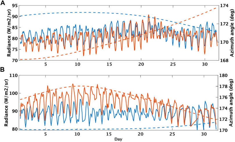
FIGURE 3. Comparison of global daytime mean EPIC shortwave radiances (left axis, solid lines) and relative azimuth angels (right axis, dashed lines) between 2017 and 2020 for (A) May and (B) December. Blue lines are for 2017 and red lines are for 2020.

3 Global Cloud Property Composite for EPIC

The Earth’s surface and atmosphere are anisotropic reflectors resulting in a relatively complex variation of radiance leaving the Earth as a function of the viewing and illumination angles. Thus, converting radiances from EPIC to fluxes requires the use of ADMs to account for the reflectance anisotropies. We use the most comprehensive ADMs developed by the CERES team (Su et al., 2015a) and these ADMs are functions of scene types defined using many variables (i.e., surface type, cloud amount, cloud phase, cloud optical depth, etc). The EPIC cloud composite was developed to provide scene identifications for each EPIC pixel to determine the anisotropy factors (Khlopenkov et al., 2017; Su et al., 2018, 2020). The composite data include cloud property retrievals from multiple imagers on low Earth orbit (LEO) satellites (including MODIS, VIIRS, and AVHRR) and geostationary (GEO) satellites (including GOES-13, -15, -16, and -17, METEOSAT-8, -9, -10, and -11, MTSAT-2, and Himawari-8). All cloud properties were determined using a common set of algorithms, the Satellite ClOud and Radiation Property retrieval System (SatCORPS, Minnis et al., 2008a, 2016), based on the CERES cloud detection and retrieval system (Minnis et al., 2008b, 2011; 2010; Trepte et al., 2019). Cloud properties from these LEO/GEO imagers are optimally merged together to provide a seamless global composite product at 5-km resolution by using an aggregated rating that considers five parameters (nominal satellite resolution, pixel time relative to the EPIC observation time, viewing zenith angle, distance from day/night terminator, and Sun glint factor to minimize the usage of data taken in the glint region) and selects the best observation at the time nearest to the EPIC measurements. The global composite data are then remapped into the EPIC field of view by convolving the high-resolution cloud properties with the EPIC point spread function (PSF) defined with a half-pixel accuracy to produce the EPIC composite. PSF-weighted averages of radiances and cloud properties are computed separately for each cloud phase, because the LEO/GEO cloud products are retrieved separately for liquid and ice clouds (Minnis et al., 2008a). Ancillary data (i.e. surface type, snow and ice map, skin temperature, precipitable water, etc.) needed for anisotropic factor selections are also included in the EPIC composite. These composite images are produced for each observation time of the EPIC instrument (typically 300 to 600 composites per month).

Figure 4 shows retrieved liquid and ice cloud properties for January 4, 2017 at 11:15 UTC. The EPIC RGB image taken at this time is shown in Figure 5. At this image time, 56% of the daytime portion of the Earth is covered by clouds and about 2/3 of the clouds are of liquid phase. The optical depths of liquid clouds are mostly less than 6, but there are some very thick clouds with optical depth exceeding 22 in the Southern Ocean. The effective cloud heights of these liquid clouds are between ∼ 1 and 6 km and the effective radii are less than 25 μm. The optical depths of ice clouds are of similar magnitude as liquid clouds. As expected, the ice clouds are higher and with larger radii than liquid clouds.

FIGURE 4

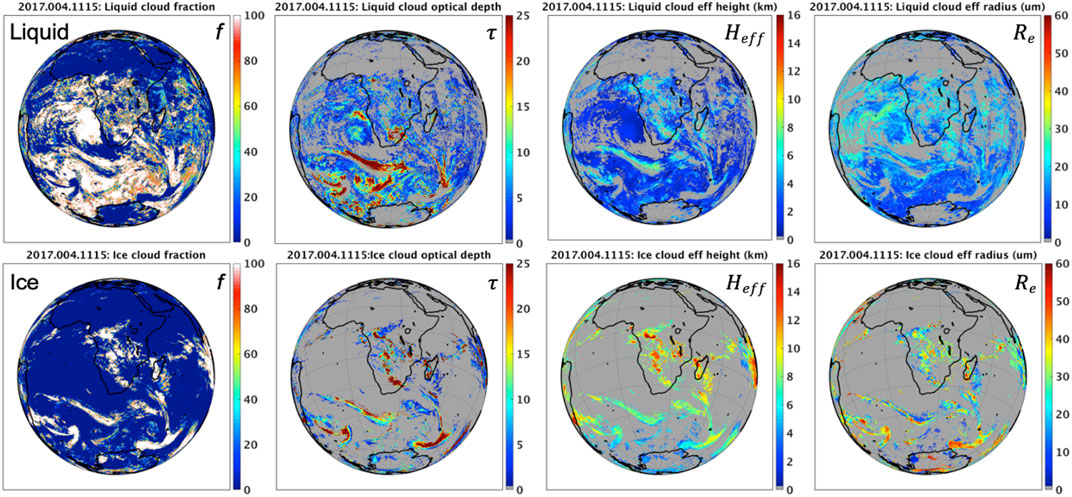
FIGURE 4. Cloud properties retrieved from the LEO/GEO EPIC composite for January 4, 2017 at 11:15 UTC. Figures from left to right show cloud fraction (%), cloud optical depth, cloud effective height (km), and cloud effective droplet radius (μm) for liquid phase clouds (top row) and ice phase clouds (bottom row).

FIGURE 5

FIGURE 5. The RGB image from EPIC observation taken at 11:15 UTC on January 4, 2017.

Cloud fractions for the EPIC pixels can be averaged to provide the global daytime mean cloud fraction ($\overline{f_d}$) at each EPIC image time. Figure 6 shows $\overline{f_d}$ at each EPIC image time for May and December using data from 2017 to 2020. Strong diurnal cycle is evident for $\overline{f_d}$, this is because the sunlit side of the Earth is centered over the Pacific Ocean where clouds are prevalent during earlier UTC hours and centered over Africa where there are few clouds over Sahara desert around 12 UTC. Cloud fractions within the EPIC views are a few percent higher in December than in May. This is because the very cloudy Southern Ocean and Antarctic are not within the EPIC view in May. The overall $\overline{f_d}$ are fairly consistent from year to year, though there are some small variations in $\overline{f_d}$ due to transient weather systems. Thus, cloud change is not the cause for the large variations of $\overline{I_{sw}}$ shown in Figure 3.

FIGURE 6

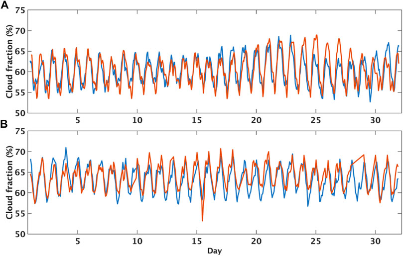
FIGURE 6. Comparison of global daytime mean cloud fraction derived from EPIC composite between 2017 and 2020 for (A) May and (B) December. Blue lines are for 2017 and red lines are for 2020.

4 Angular Distribution Models

Angular distribution models (ADMs) describe the relationship between radiance (I) and flux (F):

$F({\theta }_0,\chi )=\frac{\pi I({\theta }_0,\theta ,\varphi ,\chi )}{R({\theta }_0,\theta ,\varphi ,\chi )},(1)$

where θ₀ is the solar zenith angle, θ is the satellite viewing zenith angle, ϕ is the relative azimuth angle between the instrument and the solar plane, and R is the anisotropic factor that relates radiance to flux. For isotropic surfaces, the radiance does not depend on viewing geometry (θ, ϕ) and R is reduced to one for all viewing geometry. However, all surfaces on Earth exhibit anisotropic characteristics that can vary drastically from one scene to another which make determining the radiative flux from radiance measurement very challenging. Thus, quantifying the relationships between radiance and flux over different scene types is a critical part of determining fluxes from satellite radiance measurements.

Currently the most comprehensive ADMs available are the ones developed by the CERES team (Loeb et al., 2005; Su et al., 2015a). Realizing the importance of quantifying the anisotropies over different scene types and the deficiencies of the 12 scene-type ADMs developed for ERBE (Suttles et al., 1988), the CERES instruments are designed to fly together with an imager (MODIS for Terra and Aqua) and are also equipped with a special rotating azimuth plan (RAP) scan mode (Wielicki et al., 1996). When an instrument is placed in RAP mode, the instrument scans in elevation as it rotates in azimuth, thus acquiring radiance measurements from a wide range of viewing combinations. There are two CERES instruments on Terra and Aqua. At the beginning of their missions, one of the CERES instruments was always placed in RAP mode to maximize the angular coverage, while the other instrument was in cross track mode to maximize the spatial coverage. Figure 7 shows the logarithm sample number distributions using Aqua flight model 3 (in RAP mode) and Aqua flight model 4 (in cross track mode) observations of April 2004 when solar zenith angles are between 40^◦ and 50^◦. When CERES instrument is placed in RAP mode, the observations are almost evenly distributed across all (θ, ϕ) bins, except when θ > 80^◦. However, when CERES instrument is in cross track mode, the observations are concentrated in limited side-scattering angular bins. The sample distributions of RAP and cross-track mode are very similar for other solar zenith angle ranges. Figure 7 illustrates the critical role that RAP scan mode plays in collecting data for developing R(θ₀, θ, ϕ). It also indicates that only a small angular fraction of R(θ₀, θ, ϕ) is used in the CERES radiance-to-flux conversion.

FIGURE 7

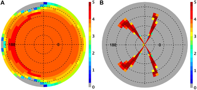
FIGURE 7. Logarithm of sample numbers in each 5^◦ viewing zenith angle and 5^◦ relative azimuth angle bin of all observations within 40^◦ and 50^◦ solar zenith angles for the Aqua CERES instrument in RAP mode (A) and in cross track mode (B) using data of april 2004. Grey color indicates no observations.

As mentioned early, DSCOVR at the L1 point observes the Earth in near-backscattering directions and offers a testbed for the CERES ADMs in these unique directions. Su et al. (2018) used the CERES ADMs and the scene identification provided by the EPIC cloud composite product to derive the global daytime mean anisotropy factors to convert the global daytime mean radiances to fluxes. They derived the EPIC SW fluxes for 2017. These fluxes agree with those derived from CERES synoptic products to within ±2% and demonstrate that the CERES ADMs accurately account for the Earth’s anisotropy in the near-backscatter direction.

Note the relative azimuth angles range between about 170^◦ and 174^◦ during 2017, whereas the relative azimuth angles can be as large as 178^◦ during 2020 (see Figure 2). As the EPIC observation moves closer to the due backscattering directions, the radiance anisotropy increases for liquid cloud due to glory feature and for clear vegetated surface due to hot spot feature (Gatebe and King, 2016). CERES ADMs capture these changes when viewing geometries move from near-backscattering directions to backscattering directions. Figure 8 shows how anisotropic factors change as the relative azimuth angle moves from 170^◦ (near backscatter) to 179^◦ (backscatter) for clear cropland (a) and water clouds over ocean (b). For clear cropland, the CERES ADMs are constructed using the Ross-Li model (Roujean et al., 1992; Li and Strahler, 1992) that accounts for the hot spot effect (Maignan et al., 2004) on regional and calendar month basis. The clear cropland anisotropic factor increases by up to 30% around θ = 40^◦ (the hot spot) when the relative azimuth angle moves from 170^◦ to 179^◦. For liquid clouds, the CERES ADMs are constructed as a function of ln (fτ) using measured radiances with an angular resolution of 2^◦ (Su et al., 2015a). Figure 8B shows the anisotropic factors for ln (fτ) = 8, they increases by up to 9% around the glory (θ = 60^◦) when the relative azimuth angle moves from 170^◦ to 179^◦.

FIGURE 8

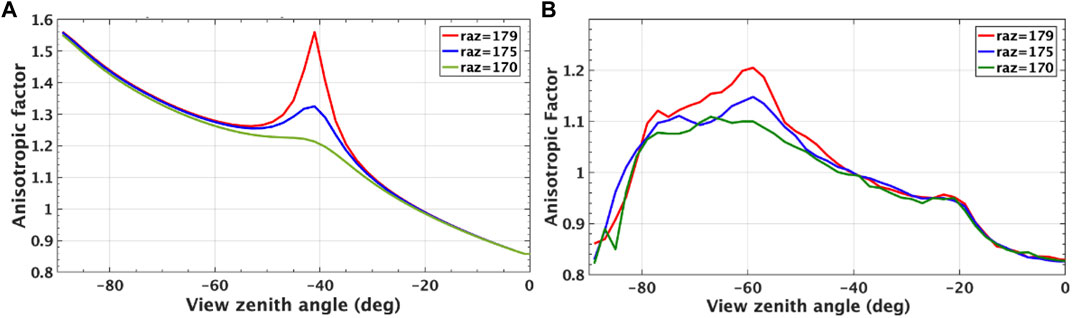
FIGURE 8. Anisotropic factors at near-backscattering directions for relative azimuth angle of 179^◦ (red), 175^◦ (blue), and 170^◦ (green) for (A) clear cropland in December with solar zenith angle of 40^◦ and (B) for liquid clouds (ln (fτ)=8) over ocean with solar zenith angle of 60^◦.

Figure 9 shows the anisotropic factors at the EPIC pixel level for December 5 for 2017 and 2020 at UTC hours around 06:00 and 11:00. As shown in Figure 3B, the relative azimuth angle for December 5, 2017 is around 170^◦ and is around 177^◦ for December 5, 2020. Shifting to larger relative azimuth angles in 2020 results in larger anisotropic factors, most notably over land regions due to the hot spot effects. For the two EPIC image times, $\overline{R_{sw}}$ are 1.343 and 1.375 for 2020 compared to 1.241 and 1.254 for 2017, representing 8–10% increase in radiance anisotropy.

FIGURE 9

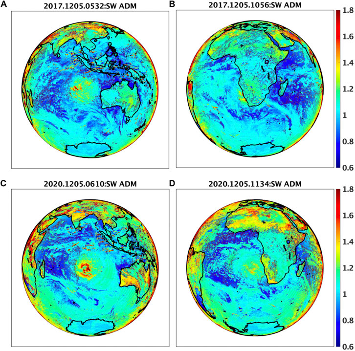
FIGURE 9. Anisotropic factors at the EPIC pixel level for December 5, 2017 (top row) at image time of 05:32 UTC (A), and 10:56 UTC (B), and for December 5, 2020 (bottom row) at image time of 06:10 UTC (C), and 11:34 UTC (D).

5 EPIC SW Flux

Using $\overline{I_{sw}}$ and $\overline{R_{sw}}$ described above, we can calculate $\overline{F_{sw}}$ for each EPIC image time. Figure 10 compares $\overline{F_{sw}}$ between 2017 and 2020 for May and December. Despite the large differences in $\overline{I_{sw}}$ between these 2 years, especially for December (see Figure 3), $\overline{F_{sw}}$ are similar. For May 2017, $\overline{F_{sw}}$ is 198.6 Wm⁻²; and for May 2020, $\overline{F_{sw}}$ is 196.5 Wm⁻². For December 2017, $\overline{F_{sw}}$ is 223.4 Wm⁻²; and for December 2020, $\overline{F_{sw}}$ is 220.1 Wm⁻².

FIGURE 10

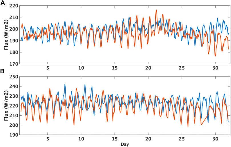
FIGURE 10. Comparison of global daytime mean EPIC shortwave fluxes between 2017 and 2020 for (A) May and (B) December. Blue lines are for 2017 and red lines are for 2020.

As there are no direct TOA flux measurements, global daytime mean SW fluxes from EPIC are compared against CERES Edition 4 Synoptic radiative fluxes and cloud product (SYN1deg, Doelling et al., 2013). SYN1deg data product provides hourly cloud properties and fluxes for each 1^◦ latitude by 1^◦ longitude. Hourly fluxes within SYN1deg are from CERES observations at the CERES overpass times and for the hours between CERES observations they are inferred from hourly GEO imager measurements. The GEO visible and infrared measurements are used to derive broadband radiances using observation-based narrowband-to-broadband regression relationships and radiance-to-flux conversion algorithms. These GEO derived fluxes are used to fill in the hour boxes between CERES observations between 60^◦S and 60^◦N. For regions in the high latitudes, CERES instruments on the polar-orbiting Terra and Aqua satellites provide sufficient temporal coverage. Several procedures are implemented to ensure the consistency between the MODIS-derived and GEO-derived cloud properties, and between the CERES fluxes and the GEO-based fluxes. These include calibrating GEO visible radiances against the well-calibrated MODIS 0.65 μm radiances by ray-matching MODIS and GEO coincident radiances; applying similar cloud retrieval algorithms to derive cloud properties from MODIS and GEO observations; and normalizing GEO-based broadband fluxes to CERES fluxes using coincident measurements (Doelling et al., 2013).

The hourly gridded SYN1deg fluxes are integrated by considering only the grid boxes that are visible to the EPIC to produce the global mean daytime fluxes that are comparable to those from the EPIC measurements following the method developed by Su et al. (2018). Figure 11 compares the global daytime mean hourly fluxes from EPIC and SYN1deg for May 2017 (a) and May 2020 (b). The biases and root-mean-square (RMS) errors are comparable for the EPIC SW fluxes for both May 2017 and May 2020, despite changes in EPIC viewing angles. For May 2017, the relative azimuth angle at the beginning of the month is 173^◦ and decreases to about 171^◦ near the end of the month. For May 2020, the relative azimuth angle starts around 168^◦ and increases to close to 174^◦ near the end of the month (see Figure 3A). Figure 12 compares the global daytime mean hourly fluxes from EPIC and SYN1deg for December 2017 (a) and December 2020 (b). Similar to the comparison results for May, both Decembers compare favorably with the global daytime fluxes from SYN1deg with the mean biases less than 0.6 W m^-2 and RMS error less than 3 W m^-2, despite that December 2020 has the largest relative azimuth angles (∼ 178^◦) seen during the entire DSCOVR observational period. Additionally, the relative azimuth angles are quite different for December 2017 and December 2020. For December 2017, the relative azimuth angle stayed close to 170^◦ until December 22 and then started to increase slightly. For December 2020, the relative azimuth angle started around 175^◦ and reached the maximum around December 10 before decreasing to about 172^◦ by the end of the month. The good agreement shown in Figures 11, 12 demonstrate that the CERES ADMs used for radiance-to-flux conversion capture the radiance anisotropy changes for EPIC observations taken at different relative azimuth angles from 168^◦ to 178^◦.

FIGURE 11

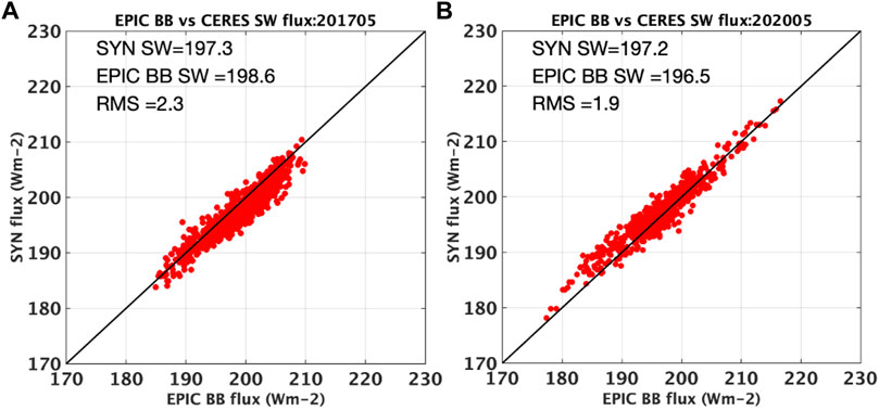
FIGURE 11. Comparison of global daytime mean shortwave flux between EPIC and CERES SYN for May 2017 (A) and May 2020 (B).

FIGURE 12

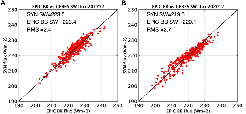
FIGURE 12. Comparison of global daytime mean shortwave flux between EPIC and CERES SYN for December 2017 (A) and December 2020 (B).

Figure 13 compares SW fluxes from CERES SYN1deg product with those from EPIC at all coincident hours of 2017–2020. Excellent agreements are found between these two datasets with the mean biases of 0.5 Wm⁻² and RMS errors less than 3 Wm⁻², despite large changes in viewing geometries (Figure 2). The SW flux agreement between these two data sets is within the uncertainties from CERES calibration, EPIC calibration, narrowband-to-broadband regression, and the angular distribution models. This comparison indicates that the method developed to calculate the global anisotropic factors from the CERES empirical ADMs using the EPIC cloud composites for scene identifications is robust and that the CERES angular distribution models accurately account for the Earth’s anisotropy in the near-backscattering to due-backscattering directions.

FIGURE 13

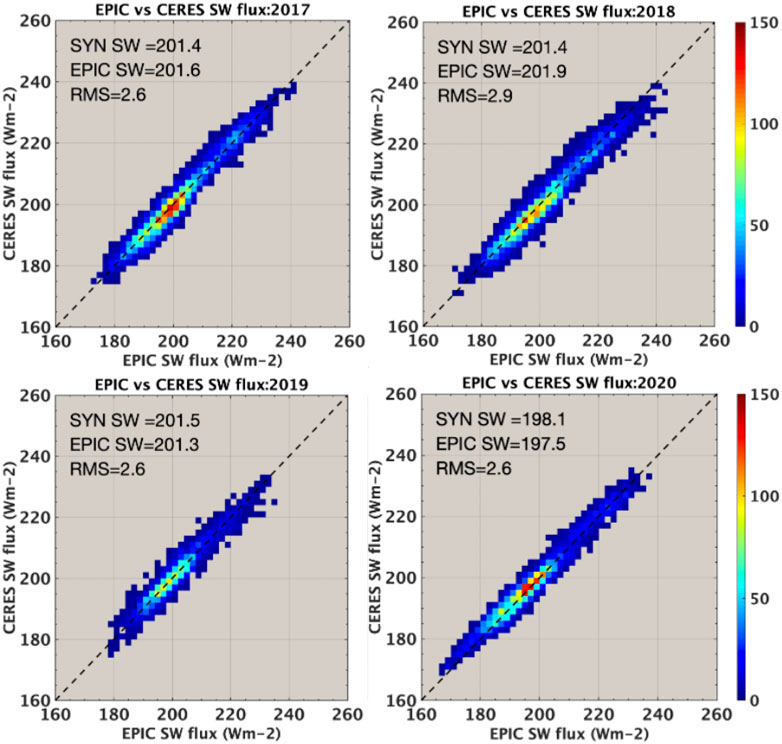
FIGURE 13. Comparison of coincident hourly SW fluxes from EPIC and CERES SYN1deg for 2017–2020.

Conclusion

DSCOVR is the first Earth-observing satellite at the Lagrange-1 (L1) point with two Earth observing instruments aim to provide continuous observations of the sunlit side of the Earth. DSCOVR is in an elliptical Lissajous orbit around the L1 point where the EPIC and NISTAR view the Earth from a small range of relative azimuth angle from 168^◦ to 178^◦. This viewing geometry is unique to EPIC as instruments (i.e., MODIS and CERES) on Terra and Aqua view the Earth mostly from side-scattering angles. Thus applying the CERES ADMs to EPIC observations offers an opportunity to test the performance of radiance-to-flux conversion in the near back-scattering angles.

Previous study by Su et al. (2018) demonstrates that the CERES ADMs accurately account for the Earth’s anisotropy using 2017 EPIC observations when the relative azimuth angle is between 170^◦ and 174^◦. However, the relative azimuth angle in 2020 shows large month-to-month variations, changing from 168^◦ to 178^◦. The SW radiances change rapidly within these angular ranges and can increase significantly for many scene types, most notably for liquid clouds and vegetated surface. EPIC observations indeed show that the global daytime mean SW radiances can increase by as much as 10% as the relative azimuth angle increases from 170^◦ to 178^◦. The increase in SW radiance is the result of EPIC viewing angle shifts closer to due-backscattering direction, and it is not because the Earth is more reflective (which could happen with significant increases of aerosols and clouds). When the anisotropies of the radiance fields are considered the resulting fluxes are very similar and do not show systematic differences.

The EPIC SW fluxes derived at different relative azimuth angles are compared against the CERES SYN1deg hourly SW fluxes. The biases of monthly mean fluxes (EPIC-SYN1deg) are less than 1.3 Wm⁻² and RMS errors are less than 2.7 Wm⁻² between EPIC and SYN1deg SW fluxes. These biases and RMS errors are independent of the EPIC viewing geometries, even for the largest relative azimuth angle differences observed between December 2017 and December 2020. The comparison is extended to include all coincident hours for data collected from 2017 to 2020. The annual global daytime mean SW fluxes from these two datasets agree to within 0.5 Wm⁻² and the RMS errors are less than 3.0 Wm⁻². This study demonstrates that the CERES ADMs capture the anisotropy changes for relative azimuth angles between 168^◦ and 178^◦. Furthermore, CERES instruments view the Earth mostly from side-scattering angles and the good agreement between global daytime mean fluxes from EPIC and CERES SYN1deg shows that fluxes inverted from different viewing angles are consistent with each other. Flux consistency is an indication that the CERES ADMs provide accurate characterization of the anisotropy for different Earth scenes and can be used for flux inversion from different viewing perspectives.

Data Availability Statement

The original contributions presented in the study are included in the article/Supplementary Material, further inquiries can be directed to the corresponding author.

Author Contributions

WS designed the study, analyzed the data, and wrote the first draft of the paper. LL analyzed the data. DD, KK, and MT produced the EPIC cloud composite data. All authors reviewed the paper.

Funding

This work was supported by NASA DSCOVR program.

Conflict of Interest

Authors LL, DD, KK, and MT were employed by the Science Systems and Applications Inc.

The remaining author declares that the research was conducted in the absence of any commercial or financial relationships that could be construed as a potential conflict of interest.

Publisher’s Note

All claims expressed in this article are solely those of the authors and do not necessarily represent those of their affiliated organizations, or those of the publisher, the editors and the reviewers. Any product that may be evaluated in this article, or claim that may be made by its manufacturer, is not guaranteed or endorsed by the publisher.

Acknowledgments

The authors thank Alexander Marshak, Steven Lorentz, YinanYu, and Alan Smith for helpful discussions on DSCOVR viewing angles.

References

Doelling, D. R., Loeb, N. G., Keyes, D. F., Nordeen, M. L., Morstad, D., Nguyen, C., et al. (2013). Geostationary Enhanced Temporal Interpolation for CERES Flux Products. J. Atmos. Oceanic Technol. 30, 1072–1090. doi:10.1175/jtech-d-12-00136.1

CrossRef Full Text | Google Scholar

Gatebe, C. K., and King, M. D. (2016). Airborne Spectral BRDF of Various Surface Types (Ocean, Vegetation, Snow, Desert, Wetlands, Cloud Decks, Smoke Layers) for Remote Sensing Applications. Remote Sensing Environ. 179, 131–148. doi:10.1016/j.rse.2016.03.029

CrossRef Full Text | Google Scholar

Li, X., and Strahler, A. H. (1992). Geometric-Optical Bidirectional Reflectance Modeling of the Discrete Crown Vegetation Canopy: Effect of crown Shape and Mutual Shadowing. IEEE Trans. Geosci. Remote Sensing 30, 276–292. doi:10.1109/36.134078

CrossRef Full Text | Google Scholar

Loeb, N. G., Kato, S., Loukachine, K., and Manalo-Smith, N. (2005). Angular Distribution Models for Top-Of-Atmosphere Radiative Flux Estimation from the Clouds and the Earth's Radiant Energy System Instrument on the Terra Satellite. Part I: Methodology. J. Atmos. Oceanic Technol. 22, 338–351. doi:10.1175/jtech1712.1

CrossRef Full Text | Google Scholar

Maignan, F., Bréon, F.-M., and Lacaze, R. (2004). Bidirectional Reflectance of Earth Targets: Evaluation of Analytical Models Using a Large Set of Spaceborne Measurements with Emphasis on the Hot Spot. Remote Sensing Environ. 90, 210–220. doi:10.1016/j.rse.2003.12.006

CrossRef Full Text | Google Scholar

Minnis, P., Bedka, K., Trepte, Q. Z., Yost, C. R., Bedka, S. T., Scarino, B., et al. (2016). “A Consistent Long-Term Cloud and Clear-Sky Radiation Property Dataset from the Advanced Very High Resolution Radiometer (AVHRR),” in Climate Algorithm Theoretical Basis Document (C-ATBD) (Asheville, NC: CDRP-ATBD-0826 Rev 1–NASA,NOAA CDR Program). doi:10.7289/V5HT2M8T

CrossRef Full Text | Google Scholar

Minnis, P., Nguyen, L., Palikonda, R., Heck, P. W., Spangenberg, D. A., Doelling, D. R., Ayers, J. K., Smith, Jr., W. L., Khaiyer, M. M., Trepte, Q. Z., Avey, L. A., Chang, F.-L., Yost, C. R., Chee, T. L., and Szedung, S.-M. (2008a). “Near-Real Time Cloud Retrievals from Operational and Research Meteorological Satellites,” in Proc. SPIE 7108, Remote Sens. Clouds Atmos. XIII, Cardiff, Wales, UK, October 13, 2008 (Wales, UK: Cardiff). doi:10.1117/12.800344

CrossRef Full Text | Google Scholar

Minnis, P., Sun-Mack, S., Trepte, Q. Z., Chang, F.-L., Heck, P. W., Chen, Y., et al. (2010). “CERES Edition 3 Cloud Retrievals,” in 13th Conference on Atmospheric Radiation (Oregon, Portland: Am. Meteorol. Soc.), Portland, Oregon, June-July 28-02, 2010.

Google Scholar

Minnis, P., Sun-Mack, S., Young, D. F., Heck, P. W., Garber, D. P., Chen, Y., et al. (2011). CERES Edition-2 Cloud Property Retrievals Using TRMM VIRS and Terra and Aqua MODIS Data-Part I: Algorithms. IEEE Trans. Geosci. Remote Sensing 49, 4374–4400. doi:10.1109/TGRS.2011.2144601

CrossRef Full Text | Google Scholar

Minnis, P., Trepte, Q. Z., Sun-Mack, S., Chen, Y., Doelling, D. R., Young, D. F., et al. (2008b). Cloud Detection in Nonpolar Regions for CERES Using TRMM VIRS and TERRA and AQUA MODIS Data. IEEE Trans. Geosci. Remote Sensing 46, 3857–3884. doi:10.1109/tgrs.2008.2001351

CrossRef Full Text | Google Scholar

Roujean, J.-L., Leroy, M., and Deschamps, P.-Y. (1992). A Bidirectional Reflectance Model of the Earth’s Surface for the Correction of Remote Sensing Data. J. Geophys. Res. 97, 20,455–20,468. doi:10.1029/92jd01411

CrossRef Full Text | Google Scholar

Su, W., Corbett, J., Eitzen, Z., and Liang, L. (2015a). Next-Generation Angular Distribution Models for Top-Of-Atmosphere Radiative Flux Calculation from CERES Instruments: Methodology. Atmos. Meas. Tech. 8, 611–632. doi:10.5194/amt-8-611-2015

CrossRef Full Text | Google Scholar

Su, W., Corbett, J., Eitzen, Z., and Liang, L. (2015b). Next-Generation Angular Distribution Models for Top-Of-Atmosphere Radiative Flux Calculation from CERES Instruments: Validation. Atmos. Meas. Tech. 8, 3297–3313. doi:10.5194/amt-8-3297-2015

CrossRef Full Text | Google Scholar

Su, W., Khlopenkov, K. V., Duda, D. P., Minnis, P., Bedka, K. M., and Thieman, M. (20172017). “Development of Multi-Sensor Global Cloud and Radiance Composites for Earth Radiation Budget Monitoring from DSCOVR,” in Remote Sensing of Clouds and the Atmosphere XXII. Editors A. Comeron, E. I. Kassianov, K. Schafer, R. H. Picard, and K. Weber (Warsaw, Poland: Proc. SPIE 10424), 10424K. doi:10.1117/12.2278645

CrossRef Full Text | Google Scholar

Su, W., Liang, L., Doelling, D. R., Minnis, P., Duda, D. P., Khlopenkov, K., et al. (2018). Determining the Shortwave Radiative Flux from Earth Polychromatic Imaging Camera. J. Geophys. Res. Atmos. 123. doi:10.1029/2018JD029390

CrossRef Full Text | Google Scholar

Su, W., Minnis, P., Liang, L., Duda, D. P., Khlopenkov, K., Thieman, M. M., et al. (2020). Determining the Daytime Earth Radiative Flux from National Institute of Standards and Technology Advanced Radiometer (NISTAR) Measurements. Atmos. Meas. Tech. 13, 429–443. doi:10.5194/amt-13-429-2020

CrossRef Full Text | Google Scholar

Suttles, J. T., Green, R. N., Minnis, P., Smith, G. L., Staylor, W. F., Wielicki, B. A., et al. (1988). Angular Radiation Models for Earth-Atmosphere System, Vol. I, Shortwave Radiation. Tech. rep., NASA RP-1184.

Google Scholar

Trepte, Q. Z., Bedka, K. M., Chee, T. L., Minnis, P., Sun-Mack, S., Yost, C. R., et al. (2019). Global Cloud Detection for CERES Edition 4 Using Terra and Aqua MODIS Data. IEEE Trans. Geosci. Remote Sensing 57, 9410–9449. doi:10.1109/TGRS.2019.2926620

CrossRef Full Text | Google Scholar

Wielicki, B. A., Barkstrom, B. R., Harrison, E. F., Lee, R. B., Louis Smith, G., and Cooper, J. E. (1996). Clouds and the Earth's Radiant Energy System (CERES): An Earth Observing System Experiment. Bull. Amer. Meteorol. Soc. 77, 853–868. doi:10.1175/1520-0477(1996)077<0853:catere>2.0.co;2

CrossRef Full Text | Google Scholar

Yang, W., Marshak, A., Várnai, T., and Knyazikhin, Y. (2018). EPIC Spectral Observations of Variability in Earth's Global Reflectance. Remote Sens (Basel) 10, 254. doi:10.3390/rs1002025410.3390/rs10020254

PubMed Abstract | CrossRef Full Text | Google Scholar