 Joanna Joiner
 Zachary Fasnacht
 Bo-Cai Gao3
94% of researchers rate our articles as excellent or good
Learn more about the work of our research integrity team to safeguard the quality of each article we publish.
Find out more
ORIGINAL RESEARCH article
Front. Remote Sens., 12 August 2021
Sec. Multi- and Hyper-Spectral Imaging
Volume 2 - 2021 | https://doi.org/10.3389/frsen.2021.721957
Satellite-based visible and near-infrared imaging of the Earth’s surface is generally not performed in moderate to highly cloudy conditions; images that look visibly cloud covered to the human eye are typically discarded. Here, we expand upon previous work that employed machine learning (ML) to estimate underlying land surface reflectances at red, green, and blue (RGB) wavelengths in cloud contaminated spectra using a low spatial resolution satellite spectrometer. Specifically, we apply the ML methodology to a case study at much higher spatial resolution with the Hyperspectral Imager for the Coastal Ocean (HICO) that flew on the International Space Station (ISS). HICO spatial sampling is of the order of 90 m. The purpose of our case study is to test whether high spatial resolution features can be captured using hyper-spectral imaging in lightly cloudy and overcast conditions. We selected one clear and one cloudy image over a portion of the panhandle coastline of Florida to demonstrate that land features are partially recoverable in overcast conditions. Many high contrast features are well recovered in the presence of optically thin clouds. However, some of the low contrast features, such as narrow roads, are smeared out in the heavily clouded part of the reconstructed image. This case study demonstrates that our approach may be useful for many science and operational applications that are being developed for current and upcoming satellite missions including precision agriculture and natural vegetation analysis, water quality assessment, as well as disturbance, change, hazard, and disaster detection.
Space-borne hyper-spectral imagers are instruments that typically have a spatial resolution of the order of 100 m or better and spectral coverage from the visible through near-infrared (NIR) and sometimes also encompassing ultraviolet (UV) and/or short-wave infrared (SWIR) wavelengths. These spectrometers are enabling a host of new science and applications. For example, the 2018 United States National Academies’ Decadal Survey identified several priorities for a hyper-spectral sensor including the monitoring of terrestrial and aquatic ecosystem physiology and health; snow and ice albedo, accumulation, and melting; active surface changes including those due to volcanic eruptions, landslides, and other hazards; and land use changes and resulting effects on fluxes of energy, water, and carbon (National Academies of Sciences, Engineering, and Medicine, 2018). Several such sensors have been or are currently flying in low Earth orbit (LEO) and more are planned for launch over the next decade. Remote sensing of the Earth’s surface with hyperspectral imagers is typically not attempted in moderately cloudy conditions. Rather, observations in overcast cloudy conditions are commonly discarded in most types of surface remote sensing with backscattered sunlight (e.g., Thompson et al., 2014). Atmospheric correction, defined as the removal of atmospheric and unwanted effects such as Rayleigh, cloud, and aerosol scattering, remains a critical part of ocean and land remote sensing algorithms (e.g., Lyapustin et al., 2011a; Lyapustin et al., 2011b; Lyapustin et al., 2012; Thompson et al., 2015; Thompson et al., 2016; Frouin et al., 2019).
Joiner et al. (2021) (hereafter referred to as J21) demonstrated that surface color (red, green, and blue components) could be recovered in cloud conditions of low to moderate optical thickness as well as in heavily loaded absorbing aerosol using satellite hyper-spectral data with a machine learning based approach and appropriate training data. The instrument they used, the Global Ozone Monitoring Experiment 2 (GOME-2), covers the UV through NIR with continuous measurements at about 0.5 nm spectral resolution. J21 completed a global training with GOME-2 using orbits taken over several training days in different seasons, viewing conditions, cloud, and aerosol conditions. The trained network was then applied globally throughout the year including days not trained on. GOME-2 provided an attractive data set to demonstrate the approach since it contains complete spectral coverage from the UV through NIR and thus other instruments with different spectral coverage and resolution could also be simulated. However, the drawback of GOME-2 for this application is its spatial resolution with nadir footprints of the order of 40 km2. Within the fairly large GOME-2 pixels, many surface spatial details are obscured. It was therefore unclear to what extent and under which conditions cloud effects blur surface imagery reconstructed at higher spatial resolution. It was also not apparent how often there were cloud gaps within the large GOME-2 pixels that allow for good quality cloud clearing in relatively homogeneous pixels.
In this work, we expand on the study of J21 to examine whether their cloud-clearing approach can be effectively applied to higher spatial resolution hyper-spectral imagers with lower spectral resolution and sampling for a scene that contains pixels for which the surface is visibly obscured. Here, we use the Hyperspectral Imager for the Coastal Ocean (HICO) that flew on the International Space Station (ISS). The results of J21 showed that their approach should work well at HICO spectral resolution and sampling. We conduct a case study over the northern coast of Florida, where there were overcast conditions over much of the scene with optically thin clouds over a portion of the scene transitioning to overcast conditions with optically thick clouds over another portion. With HICO we also examine the accuracy of the cloud-clearing at near-infrared wavelengths and show how this applies to reconstructions of a vegetation index; this was not done in the previous J21 GOME-2 study.
The basic cloud-clearing approach involves the use of an artificial neural network (NN) to retrieve surface spectral reflectances from observations in overcast skies. The approach is a spectral method of the type that has been employed for image dehazing, with far ranging applications such as search and rescue and event recognition (e.g., Mehta et al., 2020, and references therein) and ocean remote sensing in the presence of thin clouds, aerosol, and glitter (Gross-Colzy et al., 2007a; Gross-Colzy et al., 2007b; Schroeder et al., 2007; Steinmetz et al., 2011; Frouin et al., 2014). Unlike other approaches such as spatial, temporal, and non-complementation methods (e.g., Zhang et al., 2018; Wang et al., 2019; Li et al., 2019, and references therein), our methodology does not require a priori information about the Earth’s surface or atmosphere (beyond an appropriate data set for NN training). In addition to cloud effects, the observations are impacted by scattering and absorption from air molecules (Rayleigh scattering and absorption from gases such as O2, H2O, and O3). The method is able to remove these effects along with those of the clouds.
We use reflectance measurements from the United States Naval Research Laboratory’s (NRL) HICO [data provided by NASA Goddard Space Flight Center, Ocean Ecology Laboratory, Ocean Biology Processing Group (2018)]. HICO has continuous spectral coverage from approximately 400–1,000 nm with a spectral binning of ∼5.73 nm. It flew on the Japanese Experiment Module-Exposed Facility on the ISS at an altitude of approximately 350 km and at an inclination of 51.6°. HICO incorporates an Offner grating-type spectrometer that images in a pushbroom mode. The operations period was from October 1, 2009 through September 13, 2014 with a focus on coastal zones worldwide. The ground sample distance is approximately 90 m in both the cross- and along-track directions. The cross-track instantaneous field-of-view (IFOV) varies with view angle from 83 m at nadir to 182 m at 45°. In the along-track direction, the IFOV is also 83 m at nadir and increases to 120 m at 45°. The camera employs a 512 × 512 charge-coupled device (CCD). Calibration procedures are described by Lucke et al. (2011) and Gao et al. (2012).
There are a few noted issues with HICO that may affect results shown here. Second-order light from wavelengths between 350 and 540 nm falls into the same pixels as the first-order light between 700 and 1,080 nm. Although an empirical correction technique was developed (Li et al., 2012), there may still be errors in a bright cloudy scene such as the one we focus on. Imperfections in the frame smearing correction (Lucke et al., 2011) may also affect results shown here.
Here, we use two sets of observations taken over the northern coast of Florida that include a portion of the Panama City Beach area, Mexico Beach, and the St. Joseph Bay. The first scene is taken over mostly clear skies on day 78 (March 19) of 2011 (scene H2011078211654) and is used as the target or outputs for NN training. The second cloud-covered scene is from 17 days later on day 95 (April 5) (scene H2011095142905) and is used for NN inputs during the training and evaluation. A basic assumption is that the scene has not changed during the 17 days period in between when the two observations were made.
Because the two scenes are spatially mismatched, it is necessary to align them for the NN training. This was accomplished using the AUTO_ALIGN_IMAGES software provided for use in the interactive display language (IDL) by T. Metcalf. With this software, we aligned images of the difference vegetation index (DVI) defined as the NIR minus red reflectance (Tucker, 1979). The DVI provides enhanced contrast for image alignment in cloudy conditions as compared with a single wavelength as will be shown below. The DVI is also an indicator of greenness; it similar to the normalized difference vegetation index (NDVI) defined as NDVI = DVI/(NIR + red reflectance). The denominator of the NDVI provides a normalization. However, this normalization may slightly amplify noise in a reconstructed image as discussed below. This is why we use the DVI in this work rather than the NDVI.
The northernmost portion of the full scene (all pixels north of 30.45 N) was discarded because some clouds were detected on March 19 in this part of the scene which is taken to be the clear sky reference. In addition, we trimmed off the sides of the aligned images to use rows 20–479 and columns 20–1980 for training. This corresponds to latitudes between 29.59 and 30.45 N and longitudes between 85.05 and 86.42 W. For the cloudy day (April 5), the VZA range is 11.2–17.6°. For the clear day (March 19), the VZA range is 12.3–18.3° such that there was not much relative FOV distortion between the two sets of observations.
Figure 1 shows a flow diagram of the NN training that reconstructs red, green, blue, and near-infrared surface reflectances (henceforth denoted RGBNrecon or Rrecon, Grecon, Brecon, and Nrecon) from cloudy HICO reflectances ρcld. The approach is similar to that detailed in J21, however with a few minor differences. J21 used nadir-adjusted collocated reflectances derived from a different sensor, the moderate-resolution imaging spectroradiometer (MODIS), as the target in the NN training developed for GOME-2. The MODIS MCD43 data were processed over a 16 days window in order to construct surface reflectances adjusted to nadir view (Schaaf et al., 2002; Wang et al., 2018). MCD43 processing includes removal of cloudy data as well as atmospheric correction and quality control. Clear-sky data are then weighted over the 16 days window towards the day of interest. Therefore, MCD43 are somewhat smoothed over a 16 days interval. We were not able to collocate the HICO and the lower resolution MODIS images to a satisfactory level for training. Instead, we use clear sky data HICO taken on another day close in time (17 days apart) to our cloudy day of interest for the target in our NN training.
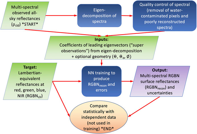
FIGURE 1. Flow diagram showing how surface reflectances at red (R), green (G), blue (B), and near-infrared (N) wavelengths are reconstructructed and their uncertainties are estimated with a neural network (NN) using hyper-spectral reflectance measurements from HICO.
Surface Lambertian-equivalent reflectances (LERs) at R, G, B, and N wavelengths are derived from the clear sky image on March 19 to be used as the predicted or target variables. The wavelengths used to define R, G, B, and N are 630–690, 520–600, 450–520, and 780–900 nm, respectively, similar to bands on the Landsat seven Enhanced Thematic Mapper Plus (ETM+). These bands are slightly wider than the Landsat eight Operational Line Sensor (OLI) and Sentinel two bands and were chosen to potentially optimize signal to noise performance though differences in performance with respect to the exact RGBN bands are expected to be small. Surface LERs are derived by inverting
where I0 is the radiance contributed by the atmosphere with a black surface, T is direct plus diffuse irradiance reaching the surface converted to an ideal Lambertian reflected radiance in the direction an observer by division by π, then multiplied by the transmittance between surface and top-of-atmosphere, and Sb is the diffuse flux reflectivity of the atmosphere for isotropic illumination from below. We compute I0, T, and Sb using the vector linearized discrete ordinate radiative transfer (VLIDORT) software (Spurr, 2006). Henceforth, R, G, B, and N will refer to LERs at red, green, blue, and NIR wavelengths, respectively.
Once trained, the non-linear NN reconstruction of RGBNrecon, denoted as fNN, can be described by
where the inputs depend on observed reflectance spectra ρcld(λ) along with the optional sun-satellite geometry that can be described by the cosines of the solar zenith, view zenith, and phase angles, θ0, θ, and ϕ, respectively.
As in J21, we reduce the dimensionality of the HICO spectra by performing a principal component analysis (PCA) or eigen-decomposition of a covariance matrix constructed from a large sample of spectra from the cloudy scene on April 5, 2011 (note that we do not subtract a mean spectrum first as is common practice for PCA). We use coefficients of the leading modes as the actual NN predictors or pseudo-observations. We also reconstruct each spectrum using the leading mode coefficients as a quality check as described below. While J21 found that 14 leading modes well captured most of the spectral variability in GOME-2 spectra, we find that 12 modes are sufficient for the lower spectral resolution HICO spectra in order to represent most of the variability (>99.9987%) in the wavelength range 400–1,000 nm.
As in J21, we find that training results improve when we remove water-contaminated pixels; the NN would require a large number of samples over many different sun-satellite geometries to effectively learn the complex angular-spectral dependencies of water surface scattering. Such an effort is beyond the scope of this case study. We use quality control filters for training data similar to those in J21 as follows: 1) to remove observations with optically thick clouds, we filter out pixels with an observed red reflectance in the cloudy scene of >0.7 (note that this check was not necessary for the cloudy scene in this study as no pixels meet this requirement); 2) to remove water-contaminated observations, we filter out pixels with observed red and NIR reflectances in the clear scene <0.1; 3) to remove suspect spectra, we check the reconstruction of each spectrum with leading modes and discard if the maximum error in the reconstructed spectrum exceeds the mean error computed over all spectra in the training set by more than 5σ. This flagging may identify erroneous observations in spectra, such as excessive amounts of scattered light or other spectral distortions (removes ∼0.2% of otherwise good pixels).
The total number of samples that meet passing all quality control checks was 180,996. We conduct the training and evaluation using two fold cross validation, where two separate trainings were conducted each using half the samples for training and the other half for evaluation. All results shown here are for the independent samples (i.e., not used in the training). Similar statistical results were obtained for the dependent and independent samples, an indication that over-training did not occur.
We employ the same NN architecture as that used by J21, consisting of a three layer feed-forward artificial NN with two hidden layers and 2N nodes in each layer, where N = 15 is the number of inputs (coefficients of 12 leading modes and cosines of three angles defining the sun-satellite geometry). For activation functions, we use a soft-sign for the first layer, a logistic (sigmoid) for the second layer, and a bent identity for the third layer. An adaptive moment estimation optimizer minimizes the error function with a learning rate of 0.1. Inputs and outputs are both scaled to produce zero means and unit standard deviations. Two NN with this structure were constructed, one to predict the surface RGBN reflectances and the other to predict its uncertainties. The target for predicting the uncertainties is the absolute value of the differences between the target and reconstructed RGBN surface reflectances as detailed in J21.
A random sample of HICO spectra is shown in Figure 2 for conditions ranging from mostly clear, with lowest reflectances in the visible wavelengths, to overcast with higher visible reflectances in the range ∼0.2 to 0.4 that correspond to cloud optical thicknesses of around five as discussed in more detail below. Major atmospheric absorption bands are seen including the O2 A band near ∼760 nm and O2 B band near 685 nm. The red edge, characterized by a rapid rise in reflectance between about 685 and 760 nm, is apparent in the land pixels. These pixels can be distinguished from those over water that have generally low NIR reflectances. The effect of Rayleigh scattering that is more prevalent at shorter (bluer) wavelengths is also seen in the spectra as an increase in reflectance from green to blue wavelengths; the surface reflectance is generally higher in the green as compared with the blue. Some defects may be present at the longest and shortest wavelengths in this range. These artifacts are not expected to degrade results as they do not fall within the ranges of the target reflectances. HICO spectra have been adjusted within the processing of the raw data to account for instrument wavelength and response function variations across its swath (also known as the spectral smile effect) as described in Gao et al. (2012).
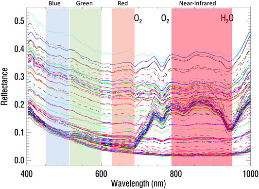
FIGURE 2. Random sampling of HICO reflectance spectra (random colors and line-types) on April 5, 2011 with major atmospheric absorption bands labeled above.
Table 1 summarizes the evaluation with statistics comparing RGBNclr and RGBNrecon. Variability captured is generally high for R, G, and B at more that 94% for these wavelengths. The r2 values are a bit lower than those reported for GOME-2 trained on collocated MODIS MCD43 data in J21 (values were about 0.98, 0.97, and 0.95 for GOME-2 reconstructed R, G, B, respectively). However, RMSD values were higher for R, G, and B for GOME-2/MODIS as compared with HICO which may result from a greater proportion of high values of reflectances contained in the global sample for GOME-2, particularly the inclusion of deserts. Note that GOME-2/MODIS r2 values decreased from red to blue wavelengths whereas the opposite behavior is seen for HICO.
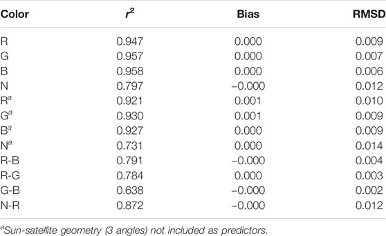
TABLE 1. Statistical comparison of reconstructed red (R), green (G), blue (B), and NIR (N) bands (RGBNrecon) and band differences with independent (not used in training) data points (180,996 in total) from the clear sky day (RGBNclr). Statistics include the root mean squared difference (RMSD), bias (mean of RGBNrecon-RGBNclr), and variance explained (r2).
As in J21, we conducted training with and without the sun-satellite angles as predictors and find that reasonable results are obtained without the geometry included (r2 > 0.92 for R, G, and B, see Table 1) though inclusion of the angles gives a small improvement. The inclusion particularly of the view angle may remove small row-dependent biases that are inherent in CCD detectors, but does not provide identifying spatial information to the neural network. Also, as in J21, we found that the errors in the reconstructed reflectances were highly correlated between the different bands. We list statistics for band differences in Table 1.
Figure 3 shows the April 5, 2011 HICO original all sky RGB image, the target surface RGB image for March 19, and the reconstructed RGB image for April 5. Here, we display only a portion of the reconstructed image that shows a gradient in cloudiness with reduced coverage over ocean (rows 1,100–1,800 and columns 200–479). The coverage corresponds approximately to latitudes between 29.59 and 30.19 N and longitudes from 85.14 to 85.77 W. The RGB images are selectively scaled using the ScaleModis procedure from the Interactive Display Language (IDL) coyote library (Fanning Software Consulting) based on original code from the MODIS rapid response team. The two images on the right and in the middle were further enhanced using the Mac Preview application with the “auto levels” function to adjust contrast.
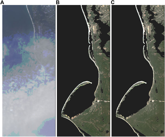
FIGURE 3. RGB imagery from HICO: (A): Original image from April 5, 2011 over the northern coast of Florida including the St. Joseph Peninsula and St. Joseph Bay. (B): Aligned image from March 19, 2011; (C): Reconstructed surface RGB using April 5 HICO spectra. Pixels over water in middle and right panels are displayed as black. See text for description of processing used to produce these images.
High reflectances over the beaches along the coastline are visible in the uppermost portion of the cloudy April 5 image where clouds are optically thin, but disappear in the lower part of the image where clouds are more optically thick. All surface features are obscured in the lower portion of the cloudy image. As will be shown below, the red reflectance in the cloudiest parts of the scene (approximately the bottom third of the scene) ranges from about 0.2 to 0.4. These reflectances correspond to cloud optical thicknesses of the order of 5 (Kujanpää and Kalakoski, 2015). Note that in the center and right panels in this figure and following figures unless otherwise noted, pixels over water surfaces, detected as described above in the March 19 clear sky image, are displayed as black as the training is not optimized for these pixels. The major bright features are fairly well captured in the reconstructed cloudy image, especially in the upper portion of the image where the clouds are more transmissive.
Figure 4 shows a similar set of panels for the DVI (NIR minus red). The DVI displays noticeable contrast between land and water scenes even through the optically thick clouds in the lower portion of the image. As in Figure 3, most of the large contrast DVI features are preserved while some of the lower contrast high spatial resolution features are washed out. Note that the DVI error due to clouds is positive in the upper part of the figure where clouds are optically thin but errors are negative in the lower portion of the scene with thicker clouds. As in Figure 3, some of the clear sky spatial features are visible in the cloudy image, while others such as in the lower portion of the image, affected by heavy clouds, are not.
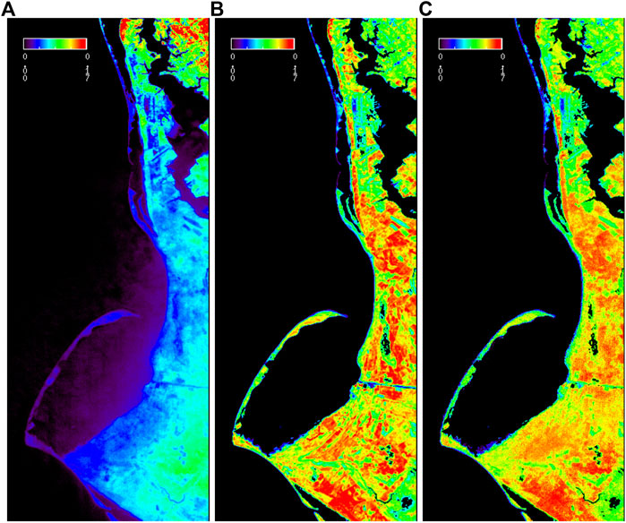
FIGURE 4. Similar to Figure 3 but for the DVI (NIR minus red): (A): Original image from cloudy April 5, 2011; (B): Original image from clear day March 19; (C): Reconstructed image from April 5. Pixels over water in middle and right panels are displayed as black.
We tested the use of standard image sharpening software packages to see whether they can be used to recover contrast and/or washed out features. This is not a part of our standard approach and results with sharpening are not shown here. We were able to restore some of the loss of contrast in the lower part of the reconstructed image in Figure 4. However, we were not able to recover additional fine scale spatial features that were lost in the reconstructed image.
In the cloudy April 5 DVI image (left panel), some moderately low values are seen extending over the ocean. The positive values do not extend in an isotropic manner around all of the coastlines as may be expected if they were due to spatial-spectral scrambling from clouds. Rather, the features over ocean appear in the direction of the image acquisition after land has been encountered. This suggests a possible ghosting effect in the readout of the CCD array. These effects would likely also occur over land and may contribute to spatial smearing. Full scene (including over ocean) clear sky images (March 19) are shown for RGB, red, and blue in Figure 5 and show that the positive DVI features over ocean in the cloudy image of Figure 4 do not correspond to those of ocean color.
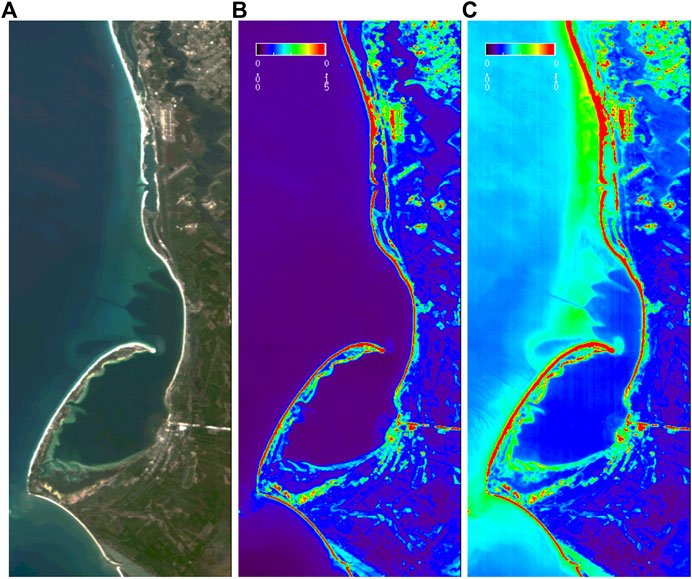
FIGURE 5. Original imagery from the clear day March 19, 2011 (ocean not blacked out); (A): RGB; (B): Red band; (C): Blue band.
Figures 6, 7 show the same set of three images as in Figures 3, 4 for the red and blue bands, respectively, along with estimated uncertainties for the reconstructed bands. As in the RGB image, the bright beaches are seen through the clouds in the upper portions of the cloudy images, but are completely obscured in the lower parts of the images. Similar to the set of images in Figures 3, 4, the high contrast features are captured fairly well, while the low contrast, high spatial features, such as roads are smeared out. Imagery appears very similar in the red and blue bands and there does not appear to be any noticeable smearing in the blue band due to increased Rayleigh scattering. Estimated uncertainties in reconstructed reflectances increase with the value of the surface reflectance similar to results shown in J21. Images in the reconstructed green band display similar features (not shown).
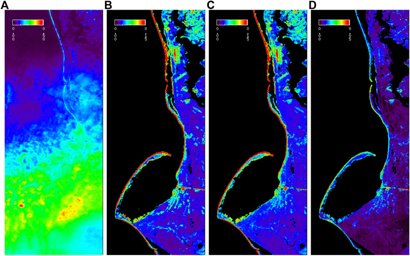
FIGURE 6. Similar to Figure 3 but for the Red band: (A): Original image from cloudy April 5, 2011; (B): Original image from clear day March 19; (C): Reconstructed image from April 5; (D): Estimated uncertainties in reconstructed reflectances. Pixels over water in middle and right panels are displayed as black.
FIGURE 7. Similar to Figure 6 but for the Blue band: (A): Original image from cloudy April 5, 2011; (B): Original image from clear day March 19; (C): Reconstructed image from April 5; (D): Estimated uncertainties in reconstructed reflectances. Pixels over water in middle and right panels are displayed as black.
While some of the low contrast, high resolution features such as roads are smeared out, particularly in the lower portion of the reconstructed imagery, it is encouraging that the higher contrast features are relatively well preserved even when the clouds appear opaque to the human eye. While we used a clear sky image over the same area for training of a neural network, none of the spatial information from the training set entered into the image reconstruction; all information used to recover the spatial-spectral details from the cloudy image came from the observed spectra on the cloudy day as well as the sun-satellite geometry.
Additional studies need to be undertaken to determine the range of conditions and instrument performance that is necessary to achieve image reconstruction with the required accuracy for a particular application. We attempted to apply the trained NN for our case study scene to other HICO scenes from different years and areas and found that it did not produce good quality RGB images. We believe this is due to the insufficiency of a limited training set. To construct a global training set with a high spatial resolution sensor such as HICO will be much more difficult and time consuming than the global training that was used in J21 with GOME-2 and MODIS. We therefore caution that the results shown here are limited in scope, and we plan to test the limits of the approach with other types of scenes and sensors in future work.
We have expanded on the work of J21 to include NIR reflectance and DVI, demonstrating that recovery of detailed vegetation information, specifically the greenness inherent in this spectral index, is possible with our reconstruction approach. The features and contrasts captured by the DVI in vegetated areas, such as man-made plots, are much more subtle in the corresponding RGB image. Therefore, applications in precision agriculture may be possible.
In our case study of a cloudy image where optically thin clouds cover the upper part of the scene transitioning to optically thick clouds (that would appear white to the human eye) in the lower portion, we demonstrate how a hyper-spectral data can be used to reconstruct much of the spatial-spectral detail that is obscured or distorted by the clouds. However, some of the highest spatial resolution features with low contrast are lost. We may attribute at least some of this loss to spectral-spatial scrambling of the observations within the optically thick clouded portion of the scene that would be expected to occur particularly in the presence of liquid water clouds. Terra MODIS data on that data indicate water clouds in the vicinity, although the Terra overpass time did not perfectly coincide (our scene was on the eastern part of the MODIS swath). Ice clouds and aerosols produce more forward scattering as compared with water clouds and therefore may produce less spectral-spatial scrambling and blurring in a reconstructed image. Our results in thin clouds shows excellent reconstruction of spectral and high spatial details. However, close inspection of our results reveals that instrumental effects may also play a significant role in the blurring of the reconstructed image. While we were not able to recover some of the fine spatial details that were lost in the blurred parts of the image with standard sharpening packages that may utilize convolutional neural networks, these sharpening tools may still useful in other scenes or with other sensors.
We note that the clear sky image was taken at 21:16 UTC or 17:16 EST which is later in the day than the cloudy image taken at 14:29 UTC or 10:29 EDT. Unlike the work of J21 that trained on many different viewing conditions with a nadir adjusted target reflectance, here we essentially neglect surface BRDF effects in the target data. Therefore, shadowing in the clear sky image may have degraded the fitting results somewhat.
This study focuses on land surfaces with a very limited training data set. More training data over a wide range of angles and conditions would be needed to effectively reconstruct imagery over the ocean surface with our methodology. We plan to address ocean applications in future works. We also plan to apply our approach to other hyperspectral imagers. In addition to HICO, there are many more current and planned hyper-spectral satellite instruments that our method could be applied to. These include the German Aerospace Center (DLR) Earth Sensing Imaging Spectrometer (DESIS) (Krutz et al., 2019), the Japanese Ministry of Economy, Trade, and Industry (METI) Hyperspectral Imager Suite (HISUI), and the NASA Earth Surface Mineral Dust Source Investigation (EMIT), all currently flying on the ISS, as well as with similar spectral coverage and GSD of ∼30 m (Krutz et al., 2019), the Italian Space Agency’s (ASI) Hyperspectral Precursor of the Application Mission (PRISMA). The next few years will see the launches of the German Environmental Mapping and Analysis Program (EnMAP) (Storch et al., 2020), the European Space Agency (ESA) Copernicus Hyperspectral Imaging Mission (CHIME), and NASA surface biology and geology (SBG) mission. Hyper-spectral instruments can also be operated from the ground or flown on airborne platforms. The techniques developed here provide capability to do remote sensing in cloudy conditions and increase the data coverage and timeliness of products from these sensors for a wide variety of applications. We plan to conduct our own testing and encourage adoption of our approach with these sensors.
The original contributions presented in the study are included in the article/supplementary material, further inquiries can be directed to the corresponding author.
JJ was responsible for the conceptualization and design of the methodology, supervision, funding acquisition, data curation, visualization, and formal analysis, and wrote the first draft of the manuscript. JJ, ZF, and WQ contributed to the software and calculations. JJ and B-CG contributed to the investigation. All authors contributed to manuscript revision, read, and approved the submitted version.
This work was supported in part by the NASA through the Arctic-Boreal Vulnerability Experiment (ABoVE) as well as the PACE and TEMPO science team programs.
ZF and WQ were employed by Science Systems and Applications, Inc. (SSAI).
The remaining authors declare that the research was conducted in the absence of any commercial or financial relationships that could be construed as a potential conflict of interest.
All claims expressed in this article are solely those of the authors and do not necessarily represent those of their affiliated organizations, or those of the publisher, the editors and the reviewers. Any product that may be evaluated in this article, or claim that may be made by its manufacturer, is not guaranteed or endorsed by the publisher.
We are particularly grateful to the NRL HICO team and the NASA ocean data distribution team for making available high quality HICO data. The lead author thanks P. K. Bhartia, A. da Silva, L. Remer, and two reviewers for enlightening comments that helped to improve the manuscript.
Frouin, R., Duforêt, L., and Steinmetz, F. (2014). “Atmospheric Correction of Satellite Ocean-Color Imagery in the Presence of Semi-transparent Clouds,” in Ocean Remote Sensing and Monitoring from Space. Editors R. J. Frouin, D. Pan, and H. Murakami (Bellingham, WA: International Society for Optics and Photonics (SPIE)), 9261, 47–61. doi:10.1117/12.2074008
Frouin, R. J., Franz, B. A., Ibrahim, A., Knobelspiesse, K., Ahmad, Z., Cairns, B., et al. (2019). Atmospheric Correction of Satellite Ocean-Color Imagery during the PACE Era. Front. Earth Sci. 7, 145. doi:10.3389/feart.2019.00145
Gao, B.-C., Li, R.-R., Lucke, R. L., Davis, C. O., Bevilacqua, R. M., Korwan, D. R., et al. (2012). Vicarious Calibrations of HICO Data Acquired from the International Space Station. Appl. Opt. 51, 2559–2567. doi:10.1364/AO.51.002559
Gross-Colzy, L., Colzy, S., Frouin, R., and Henry, P. (2007a). “A General Ocean Color Atmospheric Correction Scheme Based on Principal Components Analysis: Part I. Performance on Case 1 and Case 2 Waters,” in Coastal Ocean Remote Sensing. Editors R. J. Frouin, and Z. Lee (Bellingham, WA: International Society for Optics and Photonics (SPIE)), 6680, 9–20. doi:10.1117/12.738508
Gross-Colzy, L., Colzy, S., Frouin, R., and Henry, P. (2007b). “A General Ocean Color Atmospheric Correction Scheme Based on Principal Components Analysis: Part II. Level 4 Merging Capabilities,” in Coastal Ocean Remote Sensing. Editors R. J. Frouin, and Z. Lee (Bellingham, WA: International Society for Optics and Photonics (SPIE)), 6680, 21–32. doi:10.1117/12.738514
Joiner, J., Fasnacht, Z., Qin, W., Yoshida, Y., Vasilkov, A., Li, C., et al. (2021). Use of Multi-Spectral Visible and Near-Infrared Satellite Data for Timely Estimates of the Earth's Surface Reflectance in Cloudy and Aerosol Loaded Conditions: Part 1 - Application to RGB Image Restoration over Land with GOME-2. EarthArXiv. doi:10.31223/X5JK6H
Krutz, D., Müller, R., Knodt, U., Günther, B., Walter, I., Sebastian, I., et al. (2019). The Instrument Design of the DLR Earth Sensing Imaging Spectrometer (DESIS). Sensors 19, 1622. doi:10.3390/s19071622
Kujanpää, J., and Kalakoski, N. (2015). Operational Surface UV Radiation Product from GOME-2 and AVHRR/3 Data. Atmos. Meas. Tech. 8, 4399–4414. doi:10.5194/amt-8-4399-2015
Li, R.-R., Lucke, R., Korwan, D., and Gao, B.-C. (2012). A Technique for Removing Second-Order Light Effects from Hyperspectral Imaging Data. IEEE Trans. Geosci. Remote Sens. 50, 824–830. doi:10.1109/TGRS.2011.2163161
Li, Z., Shen, H., Cheng, Q., Li, W., and Zhang, L. (2019). Thick Cloud Removal in High-Resolution Satellite Images Using Stepwise Radiometric Adjustment and Residual Correction. Remote Sens. 11, 1925. doi:10.3390/rs11161925
Lucke, R. L., Corson, M., McGlothlin, N. R., Butcher, S. D., Wood, D. L., Korwan, D. R., et al. (2011). Hyperspectral Imager for the Coastal Ocean: Instrument Description and First Images. Appl. Opt. 50, 1501–1516. doi:10.1364/AO.50.001501
Lyapustin, A., Martonchik, J., Wang, Y., Laszlo, I., and Korkin, S. (2011a). Multiangle Implementation of Atmospheric Correction (MAIAC): 1. Radiative Transfer Basis and Look-Up Tables. J. Geophys. Res. Atmos. 116, D03210. doi:10.1029/2010jd014985
Lyapustin, A., Wang, Y., Laszlo, I., Kahn, R., Korkin, S., Remer, L., et al. (2011b). Multiangle Implementation of Atmospheric Correction (MAIAC): 2. Aerosol Algorithm. J. Geophys. Res. Atmos. 116, D03211. doi:10.1029/2010jd014986
Lyapustin, A. I., Wang, Y., Laszlo, I., Hilker, T., G.Hall, F., Sellers, P. J., et al. (2012). Multi-angle Implementation of Atmospheric Correction for MODIS (MAIAC): 3. Atmospheric Correction. Remote Sens. Environ. 127, 385–393. doi:10.1016/j.rse.2012.09.002
Mehta, A., Sinha, H., Mandal, M., and Narang, P. (2020). Domain-aware Unsupervised Hyperspectral Reconstruction for Aerial Image Dehazing. arXiv preprint. Available at: https://arxiv.org/pdf/2011.03677.pdf.
NASA Goddard Space Flight Center, Ocean Ecology Laboratory, Ocean Biology Processing Group (2018). Sea-viewing Wide Field-Of-View Sensor (SeaWiFS) Ocean Color Data, NASA OB.DAAC. [Dataset]. (Accessed on 01 29, 2021). doi:10.5067/ORBVIEW-2/SEAWIFS/L2/OC/2018
National Academies of Sciences, Engineering, and Medicine (2018). Thriving on Our Changing Planet: A Decadal Strategy for Earth Observation from Space. [Dataset]. doi:10.17226/24938
Schaaf, C. B., Gao, F., Strahler, A. H., Lucht, W., Li, X., Tsang, T., et al. (2002). First Operational BRDF, Albedo Nadir Reflectance Products from MODIS. Remote Sens. Environ. 83, 135–148. doi:10.1016/s0034-4257(02)00091-3
Schroeder, T., Behnert, I., Schaale, M., Fischer, J., and Doerffer, R. (2007). Atmospheric Correction Algorithm for MERIS above Case‐2 Waters. Int. J. Remote Sens. 28, 1469–1486. doi:10.1080/01431160600962574
Spurr, R. J. D. (2006). VLIDORT: A Linearized Pseudo-spherical Vector Discrete Ordinate Radiative Transfer Code for Forward Model and Retrieval Studies in Multilayer Multiple Scattering Media. J. Quant. Spectrosc. Radiat. Transfer 102, 316–342. doi:10.1016/j.jqsrt.2006.05.005
Steinmetz, F., Deschamps, P.-Y., and Ramon, D. (2011). Atmospheric Correction in Presence of Sun Glint: Application to MERIS. Opt. Express 19, 9783–9800. doi:10.1364/OE.19.009783
Storch, T., Honold, H.-P., Alonso, K., Pato, M., Mücke, M., Basili, P., et al. (2020). Status of the Imaging Spectroscopy mission EnMAP with Radiometric Calibration and Correction. ISPRS Ann. Photogramm. Remote Sens. Spat. Inf. Sci. V-1-2020, 41–47. doi:10.5194/isprs-annals-V-1-2020-41-2020
Thompson, D. R., Green, R. O., Keymeulen, D., Lundeen, S. K., Mouradi, Y., Nunes, D. C., et al. (2014). Rapid Spectral Cloud Screening Onboard Aircraft and Spacecraft. IEEE Trans. Geosci. Remote Sens. 52, 6779–6792. doi:10.1109/TGRS.2014.2302587
Thompson, D. R., Gao, B.-C., Green, R. O., Roberts, D. A., Dennison, P. E., and Lundeen, S. R. (2015). Atmospheric Correction for Global Mapping Spectroscopy: ATREM Advances for the HyspIRI Preparatory Campaign. Remote Sens. Environ. Special Issue on the Hyperspectral Infrared Imager (HyspIRI). 167, 64–77. doi:10.1016/j.rse.2015.02.010
Thompson, D. R., Roberts, D. A., Gao, B. C., Green, R. O., Guild, L., Hayashi, K., et al. (2016). Atmospheric Correction with the Bayesian Empirical Line. Opt. Express 24, 2134–2144. doi:10.1364/OE.24.002134
Tucker, C. J. (1979). Red and Photographic Infrared Linear Combinations for Monitoring Vegetation. Remote Sens. Environ. 8, 127–150. doi:10.1016/0034-4257(79)90013-0
Wang, Z., Schaaf, C. B., Sun, Q., Shuai, Y., and Román, M. O. (2018). Capturing Rapid Land Surface Dynamics with Collection V006 MODIS BRDF/NBAR/Albedo (MCD43) Products. Remote Sens. Environ. 207, 50–64. doi:10.1016/j.rse.2018.02.001
Wang, T., Shi, J., Letu, H., Ma, Y., Li, X., and Zheng, Y. (2019). Detection and Removal of Clouds and Associated Shadows in Satellite Imagery Based on Simulated Radiance fields. J. Geophys. Res. Atmos. 124, 7207–7225. doi:10.1029/2018JD029960
Keywords: clouds, hyper-spectral, HICO, hyperspectral imagery, atmospheric correction
Citation: Joiner J, Fasnacht Z, Gao B-C and Qin W (2021) Use of Hyper-Spectral Visible and Near-Infrared Satellite Data for Timely Estimates of the Earth’s Surface Reflectance in Cloudy Conditions: Part 2- Image Restoration With HICO Satellite Data in Overcast Conditions. Front. Remote Sens. 2:721957. doi: 10.3389/frsen.2021.721957
Received: 07 June 2021; Accepted: 28 July 2021;
Published: 12 August 2021.
Edited by:
Vittorio Ernesto Brando, National Research Council (CNR), ItalyCopyright © 2021 Joiner, Fasnacht, Gao and Qin. This is an open-access article distributed under the terms of the Creative Commons Attribution License (CC BY). The use, distribution or reproduction in other forums is permitted, provided the original author(s) and the copyright owner(s) are credited and that the original publication in this journal is cited, in accordance with accepted academic practice. No use, distribution or reproduction is permitted which does not comply with these terms.
*Correspondence: Joanna Joiner, am9hbm5hLmpvaW5lckBuYXNhLmdvdg==
Disclaimer: All claims expressed in this article are solely those of the authors and do not necessarily represent those of their affiliated organizations, or those of the publisher, the editors and the reviewers. Any product that may be evaluated in this article or claim that may be made by its manufacturer is not guaranteed or endorsed by the publisher.
Research integrity at Frontiers
Learn more about the work of our research integrity team to safeguard the quality of each article we publish.