Improved Lorenz-Mie Look-Up Table for Lidar and Polarimeter Retrievals

Lidar and polarimeter aerosol microphysical retrievals require calculating single-scattering properties that are computationally expensive. One of the easiest ways to speed up these calculations is to use a look-up table. Two important currently available look-up tables were created about 15 years ago. Advancements in modern computational hardware allows us to create a new look-up table with improved precision over a larger range of aerosol properties. In this new and improved Lorenz-Mie look-up table we tabulate the light scattering by an ensemble of homogeneous isotropic spheres at arbitrary wavelengths starting from $0.355\mathit{\mu }\text{m}$. The improved look-up table covers spherical atmospheric aerosols with radii in the range of 0.001–$100\mathit{\mu }\text{m}$, with real parts of the complex refractive index in the range of 1.29–1.65, and with imaginary parts of the complex refractive index in the range of 0–0.05. We test twelve wavelengths from 0.355 to $2.264\mathit{\mu }\text{m}$ and find that the elements of the normalized scattering matrix as well as the asymmetry parameter, the aerosol absorption, backscatter, extinction, and scattering coefficients are precise to within $1\text{\%}$ for $99.99\text{\%}$ of cases. The look-up table together with C++, Fortran, Matlab, and Python codes are freely available online.

1 Introduction

Recently there is a growing interest in combining simultaneous lidar and polarimeter measurements to perform retrievals of vertically-resolved aerosol properties. For example, it is expected that the combination of lidar and polarimeter observations will significantly reduce uncertainties in aerosol radiative forcing (National Academies of Sci, 2018).

In remote sensing, lidars are active instruments that can contribute a highly accurate assessment of the vertically-resolved distribution of atmospheric aerosols. There are many different types of lidars, but our Lorenz-Mie look-up table (LUT) unit tests focus on the NASA LaRC airborne second-generation high spectral resolution lidar (HSRL-2), which makes three-wavelength lidar measurements of the atmosphere (Burton et al., 2018). HSRL-2 measurements result in the aerosol backscatter and extinction coefficients at wavelengths 0.355 (UV) and $0.532\mathit{\mu }\text{m}$ (VIS) accompanied by the attenuated backscatter coefficient at $1.064\mathit{\mu }\text{m}$.

Polarimeters are passive sensors that have greater sensitivity to the absorption properties of aerosols, but the sensitivity to vertical distribution is limited. There are many different polarimeters too, but our unit tests focus on the channels provided by the airborne NASA GISS Research Scanning Polarimeter (RSP) (Cairns et al., 1999). The RSP has nine spectral channels that are divided into two groups based on the type of detector used: visible/near infrared bands at 0.41, 0.469, 0.555, 0.67, 0.864, and $0.96\mathit{\mu }\text{m}$, accompanied by shortwave infrared bands at 1.594, 1.88, and $2.264\mathit{\mu }\text{m}$.

Retrievals of aerosol microphysical properties using lidar and polarimeter data separately or combined require significant light single-scattering calculations that can consume a majority of the computational time. In this paper, we describe the improved LUT (which we call: SIR LUT) that uses scale invariance rule (SIR) built on Mishchenko (Mishchenko, 2006) to speed up these calculations with a precision target of $1\text{\%}$ for all the optical properties. We also target the accuracy (bias) to be negligible compared to precision. The $\pm 1\text{\%}$ precision was imposed to reduce forward model errors in modeling state-of-the-art airborne lidar and polarimeters, as well as the next generation of satellite polarimetric sensors.

The fundamental design of this Lorenz-Mie LUT for lidar and polarimetric sensors builds on the spherical kernels LUT (SK LUT) (Dubovik and King, 2000; Dubovik et al., 2002a; Dubovik et al., 2006). The SK LUT is already well established and has multiple applications including but not limited to AERONET (Dubovik et al., 2006), GRASP (Dubovik et al., 2011; Dubovik et al., 2014), and many others. The SIR LUT thus represents an improvement of a previously developed approach, but we also describe its methodology in detail to further document this powerful approach and to highlight its beauty, elegance and simplicity. While using the same theoretical underpinnings, we used modern computing resources to calculate a significantly more precise LUT which we share with the community. Simulation tests show that precision of SIR LUT for all optical properties always exceeds that of SK LUT by up to $34\text{\%}$.

Throughout this paper, we will follow the notation used by Dubovik et al. (2006). Our LUT targets spherical aerosols, i.e., Lorenz-Mie scattering theory is applied (Van de Hulst, 1981; Bohren and Huffman, 1983; Mishchenko et al., 2002), but this theoretical approach can also be extended to non-spherical aerosols (Dubovik and King, 2000; Dubovik et al., 2002a; Dubovik et al., 2006; Dubovik et al., 2011; Dubovik et al., 2014).

2 Scattering Matrix and Optical Coefficients

A unit test framework was developed to test the following list of aerosol inherent optical properties (IOPs) that we target for fast and precise estimation.

The normalized matrix that relates the incident and the scattered Stokes parameters in the standard Lorenz-Mie theory of light scattering by homogeneous isotropic spheres can be represented as (Van de Hulst, 1981; Bohren and Huffman, 1983; Mishchenko et al., 2002):

$\mathbf{P}\left(\text{Θ},m,\lambda \right)=\left[\begin{array}{cccc}{P}_{11}(.)& P_{12}(.)& 0& 0\\ P_{12}(.)& P_{11}(.)& 0& 0\\ 0& 0& P_{33}(.)& P_{34}(.)\\ 0& 0& -P_{34}(.)& P_{33}(.)\end{array}\right],(1)$

where $\text{Θ}$ is the scattering angle in the range from $0^{\circ }$ to ${180}^{\circ }$, λ is the wavelength $\left(\mu \text{m}\right)$, and $m=m_{\text{R}}-i·m_{\text{I}}$ is the complex refractive index (CRI) consisting of the real part $m_{\text{R}}$ (no unit) and the imaginary part $m_{\text{I}}$ (n.u.).

The four independent elements of the normalized scattering matrix $\mathbf{P}\left(\text{Θ},m,\lambda \right)$ can be computed for each vertically-resolved atmospheric layer as

$P_{ii\prime }\left(\Theta ,m,\lambda \right)=\frac{1}{\text{sca}\left(m,\lambda \right)}{\displaystyle {\int }_{r_{\text{min}}}^{r_{\text{max}}}{C}_{ii\prime }\left(\Theta ,m,\lambda ,r\right)n\left(r\right)\text{d}r},(2)$

where r is the particle radius $\left(\mu \text{m}\right)$, $n\left(r\right)=\text{d}N\left(r\right)/\text{d}r$ is the particle size distribution (PSD) function $\left(\mu {\text{m}}^{-1}{\text{cm}}^{-3}\right)$ such that $n\left(r\right)\text{d}r$ represents the number of particles with radius between r and $r+\text{d}r$ per ${\text{cm}}^3$ of air, and $N\left(r\right)$ is the number of particles per ${\text{cm}}^3$ in the size range $\left[0,r\right]$, i.e., $N\left(r\right)={\displaystyle {\int }_0^{r}n\left(r^{\text{*}}\right)\text{d}{r}^{\text{*}}}$ (Seinfeld and Pandis, 2006). The terms $C_{ii\prime }\left(\text{Θ},m,\lambda ,r\right)=\pi r^2{Q}_{ii\prime }\left(\text{Θ},m,\lambda ,r\right)\left({\text{m}}^2{\text{sr}}^{-1}\right)$ describe the directional scattering cross sections corresponding to matrix elements $P_{ii\prime }\left(\text{Θ},m,\lambda \right)\left({\text{sr}}^{-1}\right)$ with subscript $ii\prime =\left\{\mathrm{11,12,33,34}\right\}$, whereas $Q_{ii\prime }\left(\text{Θ},m,\lambda ,r\right)\left({\text{sr}}^{-1}\right)$ describe the directional efficiencies, and $\pi r^2\left({\text{m}}^2\right)$ is the geometrical cross section (Van de Hulst, 1981; Bohren and Huffman, 1983; Mishchenko et al., 2002). In the ideal case, the integration should be done over the radius range from $r_{\text{min}}=0$ to $r_{\text{max}}=\infty$, but a non-zero $r_{\text{min}}$ and a finite value of $r_{\text{max}}$ must be chosen for numerical computations.

As a reminder, the aerosol lidar backscatter coefficient $\beta \left(m,\lambda \right)\left({\text{Mm}}^{-1}{\text{sr}}^{-1}\right)$ can be computed as

$\begin{array}{l}\beta \left(m,\lambda \right)=\frac{1}{4\pi }{\displaystyle {\int }_{r_{\text{min}}}^{r_{\text{max}}}{C}_{11}\left(180\mathrm{°},m,\lambda ,r\right)n\left(r\right)\text{d}r}\\ =\frac{\text{sca}\left(m,\lambda \right)P_{11}\left(180\mathrm{°},m,\lambda \right)}{4\pi }.\end{array}(3)$

The aerosol scattering coefficient $\text{sca}\left(m,\lambda \right)\left({\text{Mm}}^{-1}\right)$ that appears in Eqs. 2, 3 and the aerosol extinction coefficient $\alpha \left(m,\lambda \right)\left({\text{Mm}}^{-1}\right)$ can be computed as

$\left\{\text{sca},\alpha \right\}\left(m,\lambda \right)={\displaystyle {\int }_{r_{\min }}^{r_{\max }}{C}_{\text{sca},\alpha }\left(m,\lambda ,r\right)n\left(r\right)\text{d}r},(4)$

where $C_{\text{sca},\alpha }\left(m,\lambda ,r\right)=\pi r^2{Q}_{\text{sca},\alpha }\left(m,\lambda ,r\right)\left({\text{m}}^2\right)$ is a scattering (extinction) cross section and $Q_{\text{sca},\alpha }\left(m,\lambda ,r\right)$ (n.u.) is a corresponding efficiency (Van de Hulst, 1981; Bohren and Huffman, 1983; Mishchenko et al., 2002).

The aerosol absorption coefficient $\left({\text{Mm}}^{-1}\right)$ is another valuable aerosol IOP to be computed as

$\text{abs}\left(m,\lambda \right)=\alpha \left(m,\lambda \right)-\text{sca}\left(m,\lambda \right).(5)$

The ensemble-averaged asymmetry parameter (n.u.) finalizes our list of aerosol optical properties to be tested by our unit test framework:

$\langle \text{cos}\left(m,\lambda \right)\rangle =\frac{1}{2}{\displaystyle {\int }_{0^{°}}^{{\mathrm{180}}^{°}}{P}_{11}\left(\Theta ,m,\lambda \right)\sin \Theta \cos \Theta \text{d}\Theta },(6)$

where the $P_{11}\left(\text{Θ},m,\lambda \right)$ element of the normalized scattering matrix P [see Eq. 1] is traditionally referred to as the phase function and the division by $\text{sca}\left(m,\lambda \right)$ in Eq. 2 ensures that the following normalization condition is satisfied:

$\frac{1}{2}{\displaystyle {\int }_{0\mathrm{°}}^{180\mathrm{°}}{P}_{11}\left(\text{Θ},m,\lambda \right)\sin \text{Θ}\text{dΘ}=1}.(7)$

We already mentioned that precise computation of the elements of the normalized scattering matrix P [see Eq. 1] and accompanying single-scattering properties [see Eqs. 3–6] requires significant amount of time. For the purpose of retrieval of aerosol microphysical properties, it is convenient to find an efficient way to compute all these aerosol IOPs to within $\pm 1\text{\%}$ precision using a precomputed LUT.

3 Principles of Look-Up Table

In order to reduce the size of the dataset that must be stored in computer memory, the LUT takes advantage of features that are universal and allow us to develop and apply a generalized approach for all the tabulated IOPs.

One can see that Eqs. 2–4 share some commonality. The core structure of these equations can be generalized as

$\begin{array}{l}p={\displaystyle {\int }_{r_{\min }}^{r_{\max }}{C}_p(.)n\left(r\right)\text{d}r}={\displaystyle {\int }_{r_{\min }}^{r_{\max }}{C}_p(.)\frac{\text{d}N\left(r\right)}{\text{d}\ln r}\text{d}\ln r}\\ ={\displaystyle {\int }_{r_{\min }}^{r_{\max }}\frac{C_p(.)}{\frac{4}{3}\pi r^3}\frac{\text{d}V\left(r\right)}{\text{d}\ln r}\text{d}\ln r},\end{array}(8)$

where $p=\left\{P_{ii\prime }\left(\text{Θ},m,\lambda \right),\beta \left(m,\lambda \right),\text{sca}\left(m,\lambda \right),\alpha \left(m,\lambda \right)\right\}$. The other common feature of Eqs. 2–4 is that it is optimal to perform the numerical integration on a logarithmic scale because it is often assumed in atmospheric sciences that the PSD $n\left(r\right)=\text{d}N\left(r\right)/\text{d}r$ has lognormal shape (Seinfeld and Pandis, 2006). The cross sections $C_p\left(\dots ,r\right)=\pi r^2{Q}_p\left(\dots ,r\right)$ are also often plotted and analyzed on a logarithmic scale because they exhibit smoother variability in equal relative steps $\text{Δ}r/r$ (i.e., in equal logarithmic steps, since $\text{d}r/r=\text{d}\text{ln}r$) rather than in equal absolute steps $\text{Δ}r$ (Dubovik et al., 2006).

In Eq. 8 we used

$\frac{\text{d}N\left(r\right)}{\text{d}\ln r}=r\frac{\text{d}N\left(r\right)}{\text{d}r}=rn\left(r\right),(9)$

$\frac{\text{d}V\left(r\right)}{\text{d}\ln r}=\frac{4}{3}\pi r^3\frac{\text{d}N\left(r\right)}{\text{d}\ln r}=v\left(r\right)\frac{\text{d}N\left(r\right)}{\text{d}\ln r},v\left(r\right)=\frac{4}{3}\pi r^3,(10)$

and switched to the volume distribution $\text{d}V\left(r\right)/\text{d}\ln r$ because, as a rough approximation of atmospheric conditions, aerosol PSDs are equipartitioned in volume (Thomalla and Quenzel, 1982). In addition, light scattering by an ensemble of small particles depends on the particle surface area or volume rather than on the number concentration (Van de Hulst, 1981; Bohren and Huffman, 1983; Mishchenko et al., 2002).

Let us split the finite range of radii $\left[r_{\text{min}},r_{\text{max}}\right]$ into a set $\left\{r_j\right\}$ consisting of $\text{M}\gg 1$ grid bins that are logarithmically equidistant and distributed between $r_1=r_{\text{min}}$ and $r_{\text{M}}=r_{\text{max}}$ with a constant step size $\text{Δ}\ln r=\left(\ln r_{\text{M}}-\ln r_1\right)/\left(\text{M}-1\right)$. Now we can reduce the integral of Eq. 8 to its approximation by a finite sum (Twomey, 1977):

$p={\displaystyle {\int }_{r_{\min }}^{r_{\max }}\frac{C_p(.)}{v\left(r\right)}\frac{\text{d}V\left(r\right)}{\text{d}\ln r}}\text{d}\ln r\approx {\displaystyle \sum _{j=1}^{\text{M}}{C}_{p,j,\lambda }\frac{\text{d}V\left(r_j\right)}{\text{d}\ln r}}.(11)$

Equation 11 is based on the assumption that the PSD $\text{d}V\left(r\right)/\text{d}\ln r$ is a smooth function of $\text{ln}r$ and can be quadratically approximated within the narrow range $r_{j-1}\le r\le r_{j+1}$ of discrete radii on a logarithmic scale. We would like to emphasize that for improved precision we use the quadratic approximation $a_j+b_j\ln r+c_j{\text{ln}}^{2}r$ of the PSD instead of the linear (trapezoidal) approximation that has been used previously (Twomey, 1977; Dubovik et al., 2006). Following the original generalized procedure for the approximation of a PSD (Twomey, 1977), the quadratic coefficients $a_j$, $b_j$, and $c_j$ are computed corresponding to the volume distribution function $\text{d}V\left(r\right)/\text{d}\ln r$ at three consecutive radii $r_k=r_{j-1}$, $r_j$, and $r_{j+1}$:

$\frac{\text{d}V\left(r_k\right)}{\text{d}\ln r}=a_j+b_j\ln r_k+c_j{\ln }^2{r}_k.(12)$

Equation 12 can be expressed in terms of the quadratic approximation coefficients as

$\begin{array}{l}{a}_j=\frac{1}{2{\left(\Delta \ln r\right)}^2}[\frac{\text{d}V\left(r_{j-1}\right)}{\text{d}\ln r}\ln r_j\ln r_{j+1}\\ -2\frac{\text{d}V\left(r_j\right)}{\text{d}\ln r}\ln r_{j-1}\ln r_{j+1}+\frac{\text{d}V\left(r_{j+1}\right)}{\text{d}\ln r}\ln r_{j-1}\ln r_j],\\ b_j=\frac{1}{2{\left(\Delta \ln r\right)}^2}[-\frac{\text{d}V\left(r_{j-1}\right)}{\text{d}\ln r}\ln \left(r_j{r}_{j+1}\right)\\ +2\frac{\text{d}V\left(r_j\right)}{\text{d}\ln r}\ln \left(r_{j-1}{r}_{j+1}\right)-\frac{\text{d}V\left(r_{j+1}\right)}{\text{d}\ln r}\ln \left(r_{j-1}{r}_j\right)],\\ c_j=\frac{1}{2{\left(\Delta \ln r\right)}^2}\left[\frac{\text{d}V\left(r_{j-1}\right)}{\text{d}\ln r}-2\frac{\text{d}V\left(r_j\right)}{\text{d}\ln r}+\frac{\text{d}V\left(r_{j+1}\right)}{\text{d}\ln r}\right].\end{array}(13)$

The range $\left[r_j,r_{j+1}\right]$ makes the following contribution to the integral in Eq. 11:

${\displaystyle {\int }_{r_j}^{r_{j+1}}\frac{C_p(.)}{v\left(r\right)}\left(a_j+b_j\ln r+c_j{\ln }^{2}r\right)\text{d}\ln r}.(14)$

Equations 13 and 14 may be grouped by terms that include $\text{d}V\left(r_{j-1}\right)/\text{d}\ln r$, $\text{d}V\left(r_j\right)/\text{d}\ln r$, or $\text{d}V\left(r_{j+1}\right)/\text{d}\ln r$ (Twomey, 1977). We will focus only on the contribution of $\text{d}V\left(r_j\right)/\text{d}\ln r$ to the discretization in Eq. 11:

$\left[\begin{array}{l}\frac{\ln r_{j-1}\ln r_{j+1}}{{\left(\Delta \ln r\right)}^2}{\displaystyle {\int }_{r_j}^{r_{j+1}}\frac{C_p(.)}{v\left(r\right)}}\text{d}\ln r\\ -\frac{\text{ln}\left(r_{j-1}{r}_{j+1}\right)}{{\left(\text{Δ}\ln r\right)}^2}{\displaystyle {\int }_{r_j}^{r_{j+1}}\ln r\frac{C_p(.)}{v\left(r\right)}\text{d}\ln r}\\ +\frac{1}{{\left(\text{Δ}\ln r\right)}^2}{\displaystyle {\int }_{r_j}^{r_{j+1}}{\ln }^{2}r\frac{C_p(.)}{v\left(r\right)}\text{d}\ln r}\end{array}\right]\frac{\text{d}V\left(r_j\right)}{\text{d}\ln r}+\cdots .(15)$

The multiplicative factor $\text{d}V\left(r_j\right)/\text{d}\text{ln}r$ also contributes to the ranges $\left[r_{j-1},r_j\right]$ and $\left[r_{j+1},r_{j+2}\right]$. Adding the contributions of the three subranges, we finally can obtain the formula for coefficient $C_{p,j,\lambda }$ of Eq. 11:

$\begin{array}{l}{C}_{p,j,\lambda }=\frac{3\ln r_{j-2}\ln r_{j-1}}{8{\left(\text{Δ}\ln r\right)}^2}{\displaystyle {\int }_{r_{j-1}}^{r_j}\frac{Q_p\left(.,r,\lambda \right)}{r}\text{d}\ln r}\\ -\frac{3\ln \left(r_{j-2}{r}_{j-1}\right)}{8{\left(\text{Δ}\ln r\right)}^2}{\displaystyle {\int }_{r_{j-1}}^{r_j}\ln r\frac{Q_p\left(.,r,\lambda \right)}{r}\text{d}\ln r}\\ +\frac{3}{8{\left(\text{Δ}\ln r\right)}^2}{\displaystyle {\int }_{r_{j-1}}^{r_j}{\ln }^{2}r\frac{Q_p\left(.,r,\lambda \right)}{r}\text{d}\ln r}\\ -\frac{3\ln r_{j-1}\ln r_{j+1}}{4{\left(\text{Δ}\ln r\right)}^2}{\displaystyle {\int }_{r_j}^{r_{j+1}}\frac{Q_p\left(.,r,\lambda \right)}{r}\text{d}\ln r}\\ +\frac{3\text{ln}\left(r_{j-1}{r}_{j+1}\right)}{4{\left(\text{Δ}\text{ln}r\right)}^2}{\displaystyle {\int }_{r_j}^{r_{j+1}}\ln r\frac{Q_p\left(.,r,\lambda \right)}{r}\text{d}\ln r}\\ -\frac{3}{4{\left(\text{Δ}\ln r\right)}^2}{\displaystyle {\int }_{r_j}^{r_{j+1}}{\ln }^{2}r\frac{Q_p\left(.,r,\lambda \right)}{r}\text{d}\ln r}\\ +\frac{3\ln r_{j+1}\ln r_{j+2}}{8{\left(\text{Δ}\ln r\right)}^2}{\displaystyle {\int }_{r_{j+1}}^{r_{j+2}}\frac{Q_p\left(.,r,\lambda \right)}{r}\text{d}\ln r}\\ -\frac{3\ln \left(r_{j+1}{r}_{j+2}\right)}{8{\left(\text{Δ}\text{ln}r\right)}^2}{\displaystyle {\int }_{r_{j+1}}^{r_{j+2}}\ln r\frac{Q_p\left(.,r,\lambda \right)}{r}\text{d}\ln r}\\ +\frac{3}{8{\left(\text{Δ}\ln r\right)}^2}{\displaystyle {\int }_{r_{j+1}}^{r_{j+2}}{\ln }^{2}r\frac{Q_p\left(.,r,\lambda \right)}{r}\text{d}\ln r}.\end{array}(16)$

The values of coefficients $C_{p,j,\lambda }$ are independent of the PSD and depend only on the scattering angle $\text{Θ}$ (directional scattering), CRI m, and wavelength λ [see Eq. 16]. We switched to efficiencies $Q_p\left(.,r,\lambda \right)$ instead of cross sections $C_p\left(.,r,\lambda \right)$ for convenience in the following discussion.

The sets of coefficients $\left\{C_p\right\}$ can be computed once with high precision for the selected scattering angles (directional scattering) and CRIs, and stored as an LUT for each aerosol IOP p. Crucially, we only need to prepare these coefficients at a single “reference” wavelength ${\lambda }_{\text{r}}$ which will be chosen to be the shortest wavelength desired (see Section 4.1). Aerosol IOPs for longer wavelengths $\lambda \mathrm{\ge }{\lambda }_{\text{r}}$ can be estimated using the results at the reference wavelength and the scale invariance rule (SIR) of electromagnetic scattering (Dubovik et al., 2006; Mishchenko, 2006).

The discretization in Eq. 11 requires that the PSDs are smooth and wide enough to cover a significant number of densely distributed radii bins. In the case of narrow, steep PSDs, the discretization becomes less accurate because a strongly oscillating function $\text{d}V\left(r\right)/\text{d}\ln r$ can’t be accurately approximated by a quadratic function on a sparse grid of radii bins.

Later we will show that Eq. 16 provides an easy and elegant way to quickly compute all the aerosol IOPs of interest [see Eqs. 2–6], for a wide range of wavelengths using an LUT referenced to a single wavelength.

3.1 Lognormal Particle Size Distribution

The following numerical unit tests use a particular type of function as a PSD $n\left(r\right)$. An earlier study mathematically proved that the random process of sequential particle crushing naturally leads to a lognormal distribution of particle sizes (Kolmogorov, 1941). The monomodal lognormal PSD is experimentally confirmed to be a good approximation for the shape of naturally occurring aerosol PSDs in the atmosphere (Seinfeld and Pandis, 2006), and can be considered as an example of function $n\left(r\right)$ in Eqs. 2–4:

$n\left(r\right)=\frac{\text{d}N\left(r\right)}{\text{d}r}=\frac{n_{\text{t}}}{r\sqrt{2\pi }\ln \sigma }\text{exp}\left[-\frac{{\left(\ln r-\ln r_{\text{med}}\right)}^2}{2{\ln }^2\sigma }\right],(17)$

where $r_{\text{med}}$ describes the count median radius with respect to the number concentration distribution. The count median radius is defined as the radius above which there are as many particles as there are particles with radii below $r_{\text{med}}$. The term σ is the geometric standard deviation whereas $\ln \sigma$ is commonly referred to as the mode width, and $n_{\text{t}}$ is the total number concentration.

The same PSD on the logarithmic scale can be expressed in terms of volume [see Eq. 10] as

$\frac{\text{d}V\left(r\right)}{\text{d}\ln r}=\frac{4}{3}\pi r^3\frac{n_{\text{t}}}{\sqrt{2\pi }\ln \sigma }\exp \left[-\frac{{\left(\ln r-\ln r_{\text{med}}\right)}^2}{2{\ln }^2\sigma }\right].(18)$

In many cases it is more convenient to analyze the monomodal lognormal PSD in terms of effective radius $r_{\text{eff}}=r_{\text{med}}\exp \left(2.5{\ln }^2\sigma \right)$ and effective variance ${\nu }_{\text{eff}}=\exp \left({\ln }^2\sigma \right)-1$. Our analysis of the LUT performance (see Section 4.5) includes these two quantities. In our numerical simulations for polarimeter observables (see Section 4.7) we also will use a bimodal PSD that is a sum of the fine and coarse mode PSDs [see Eq. 18], each defined by its total number concentration, effective radius and effective variance.

However, the LUT can be used with any custom PSD that is smooth and wide enough to cover a significant number of densely distributed radii bins.

4 Look-Up Table

4.1 Selection of the Reference Wavelength

The fundamental decision in the design of the LUT is the choice of reference wavelength ${\lambda }_{\text{r}}$ used to compute the stored coefficients $\left\{C_p\right\}$ [see Eq. 16]. This choice has a theoretical and practical basis to optimize the application of the LUT.

For the reference wavelength of the LUT we decided to use the shortest wavelength among all remote sensing instruments of interest including the two mentioned in Section 1, i.e., ${\lambda }_{\text{r}}=0.355\mathit{\mu }\text{m}$. Let us justify our choice by noting that the size parameter $x=2\pi r/\lambda$ is used for all the Lorenz-Mie computations (Van de Hulst, 1981; Bohren and Huffman, 1983; Mishchenko et al., 2002). The size parameter conveniently relates the wavelength and radius such that the Lorenz-Mie scattering properties for a given radius and wavelength are the same as those at another wavelength after adjusting the radius. For example, an aerosol with a radius of $1.4\mathit{\mu }\text{m}$ observed at a wavelength $\lambda =2.264\mathit{\mu }\text{m}$ will be characterized by the same size parameter and identical Lorenz-Mie scattering properties as an aerosol with radius $\frac{0.355}{2.264}\times 1.4\approx 0.22\mathit{\mu }\text{m}$ observed at the reference wavelength ${\lambda }_{\text{r}}=0.355\mathit{\mu }\text{m}$:

$x=2\pi \frac{1.4}{2.264}=2\pi \frac{r}{\lambda }=2\pi \frac{\frac{0.355}{2.264}\cdot 1.4}{0.355}=2\pi \frac{\frac{{\lambda }_{\text{r}}}{\lambda }r}{{\lambda }_{\text{r}}}.(19)$

As a remark, Eq. 19 states that a shorter wavelength delivers a greater range of size parameters for a given range of radii.

If the CRI is fixed then Eq. 19 establishes a direct connection between the efficiencies [see Eqs. 2–4] at wavelengths λ and ${\lambda }_{\text{r}}$ (for simplicity, we assume $\lambda \mathrm{\ge }{\lambda }_{\text{r}}$) using a simple scaling in the radius domain given by

$Q_p\left(.,r,\lambda \right)=Q_p\left(.,\frac{{\lambda }_{\text{r}}}{\lambda }r,{\lambda }_{\text{r}}\right).(20)$

A direct connection between the efficiencies can also be expressed in terms of integrals using a linear scaling of the integration range as

${\displaystyle {\int }_{r_{\min }}^{r_{\max }}{Q}_p\left(.,r,\lambda \right)\text{d}\ln r}={\displaystyle {\int }_{\frac{{\lambda }_r}{\lambda }{r}_{\min }}^{\frac{{\lambda }_r}{\lambda }{r}_{\max }}{Q}_p\left(.,r,{\lambda }_{\text{r}}\right)\text{d}\ln r.}(21)$

Equations 20 and 21 are the key properties for understanding how this type of LUT works and can be seen as a practical application of the scale invariance rule (Mishchenko, 2006). Equation 21 can be verified numerically or proved analytically with the assumption that the efficiency $Q_p\left(.,r,\lambda \right)$ can be approximated as

$Q_p\left(.,r,\lambda \right)\approx \stackrel{\infty }{{\displaystyle \sum }_{j=1}}{q}_{p,j}(.)x^j,(22)$

where the appropriate coefficients $q_{p,j}(.)$ depend on the scattering angle $\text{Θ}$ (directional scattering) and the CRI m.

Let us directly compute and plot (see Figure 1) the absorption efficiency $Q_{\text{abs}}\left(m,\lambda ,r\right)=Q_{\alpha }\left(m,\lambda ,r\right)-Q_{\text{sca}}\left(m,\lambda ,r\right)$ at wavelengths 0.355 and $2.264\mathit{\mu }\text{m}$ in order to provide a graphical demonstration of Eq. 20. We will use the CRI $m=1.65-i\cdot {10}^{-5}$ that corresponds to an almost non-absorbing aerosol. Figure 1 shows that the absorption efficiencies at two selected wavelengths repeat each other with a constant scaling factor in the radius domain. The same conclusion also applies to the other types of efficiencies too [see Eqs. 2–4]. Equation 20 offers a simple way to obtain the efficiencies at longer wavelengths λ if the corresponding efficiency at a shorter reference wavelength ${\lambda }_{\text{r}}$ is already known. For example, in order to plot the absorption efficiency at $\lambda =2.264\mathit{\mu }\text{m}$ from $0^{+}$ to $1.4\mathit{\mu }\text{m}$ radius (from point A to point C of dashed line in Figure 1), we can substitute $1.4\mathit{\mu }\text{m}$ with $\frac{0.355}{2.264}\cdot 1.4\approx 0.22\mathit{\mu }\text{m}$ radius and perform an affine stretch of the precomputed efficiency at ${\lambda }_{\text{r}}=0.355\mathit{\mu }\text{m}$ (from point A to point B of solid line in Figure 1).

FIGURE 1

FIGURE 1. Normalized absorption efficiencies at wavelengths 0.355 and $2.264\mu \text{m}$ are related by a uniform scaling transformation which is a type of Euclidean affinity transformation.

From Figure 1 it is reasonable to conclude that the numerical integration over radii in Eqs. 2–4 for a given precision will require smaller integration steps at shorter wavelengths. The oscillations of the absorption efficiency at the wavelength $2.264\mathit{\mu }\text{m}$ (see Figure 1, dashed line) are noticeably less pronounced compared to the oscillations seen in the efficiency at $0.355\mathit{\mu }\text{m}$ (see Figure 1, solid line). The uniform scaling transformation is applied in the radius domain and uses only a partial range of the efficiency precomputed at the shortest wavelength. As the wavelength increases, the oscillations with radius become smoother, corresponding to a stretching of the oscillations at a shorter wavelength (see Figure 1). Smoother functions of radius are easier to precisely integrate. Thus, it is easier to numerically compute precise values in Eqs. 2–6 at a wavelength of $2.264\mathit{\mu }\text{m}$ compared to $0.355\mathit{\mu }\text{m}$. With this feature in mind, we can expect that the performance of the SIR LUT in general will also improve as the wavelength λ increases, if we choose the shortest wavelength of interest to be the reference wavelength ${\lambda }_{\text{r}}$.

Figure 1 also helps to graphically illustrate Eq. 21. For example, Eq. 21 demonstrates that integration of the absorption efficiency at a wavelength of $2.264\mathit{\mu }\text{m}$ (see Figure 1, dashed line) in the radii range from 0.7 to $1.4\mathit{\mu }\text{m}$ will result in the same value as integration at $0.355\mathit{\mu }\text{m}$ (see Figure 1, solid line) in the range from$\sim 0.11$ to $\sim 0.22\mathit{\mu }\text{m}$. Note the logarithmic scale of the vertical axis of Figure 1 during the visual analysis.

Theoretical reasoning supported by numerical simulations justify choosing the shortest wavelength as the reference wavelength ${\lambda }_{\text{r}}$. To accommodate existing and anticipated future passive and active sensors, we choose ${\lambda }_{\text{r}}=0.355\mathit{\mu }\text{m}$. Equations 20 and 21 allow us to relate the Lorenz-Mie scattering calculations at this reference wavelength to longer wavelengths for any PSD. In Section 4.4 we will benefit from using this key property.

4.2 Look-Up Table Parameters

The quadratures that define the precision of the SIR LUT, its speed and number of stored coefficients $\left\{C_p\right\}$ [see Eq. 16] are now discussed. It is clear that a reduction of stored information can have a negative effect on the precision of the SIR LUT. At the same time, it is inefficient to store redundant information that must be read and kept in RAM. The SIR LUT represents balance between the two conflicting criteria of precision and size.

4.2.1 Quadrature of Radii Grid Bins

Let us start with the quadrature of radii $\left\{r_j\right\}$ that was briefly mentioned in Section 3. Based on numerical simulations and earlier studies (Dubovik and King, 2000; Dubovik et al., 2002a; Dubovik et al., 2002b; Dubovik et al., 2006), we made a decision to use 650 logarithmically equidistant grid bins to cover a particle size range from $r_{\text{min}}={10}^{-3}$ to $r_{\text{max}}=100\mu$m: ${10}_1^{-3}$, $1.018\times {10}_2^{-3}$, $1.036\times {10}_3^{-3}$, $1.055\times {10}_4^{-3}$, $\dots$, ${98.2}_{649}$, and ${100}_{650}\mathit{\mu }\text{m}$. Most of the values are displayed after rounding. The subscripts correspond to the index j in Eq. 11, and is provided for reference purposes.

As we discussed in Section 4.1, the computation of efficiencies $Q_p(.)$ [see Eqs. 2–4] is made using the size parameter. A single size parameter value corresponds to different particle radii and wavelength pairs. If the desired radius r at wavelength $\lambda \mathrm{\ge }{\lambda }_{\text{r}}$ is known then the corresponding radius paired with ${\lambda }_{\text{r}}$ in the SIR LUT will be [see also Eq. 19]:

$r_{{\lambda }_{\text{r}}}=\frac{{\lambda }_{\text{r}}}{\lambda }r.(23)$

The exact range of sizes should be used if the optical properties at two different wavelengths are compared. Otherwise, the scattering particle systems are different. Thus, if the integration in Eqs. 2–4 at an arbitrary wavelength λ is also carried out from ${10}^{-3}$ to $100\mathit{\mu }\text{m}$, then the computations at different wavelengths would require the SIR LUT to cover the different radii range:

• from ${10}^{-3}$ to $100\mathit{\mu }\text{m}$ at $\lambda ={\lambda }_{\text{r}}=0.355\mathit{\mu }\text{m}$;

• from $\frac{0.355}{0.41}\times {10}^{-3}\approx 8.7\times {10}^{-4}$ to $\sim 87\mathit{\mu }\text{m}$ at $\lambda =0.41\mathit{\mu }\text{m}$;

• from $\sim 1.6\times {10}^{-4}$ to $\sim 16\mathit{\mu }\text{m}$ at $\lambda =2.264\mathit{\mu }\text{m}$.

One can see that the minimum radius at all wavelengths $\lambda >{\lambda }_{\text{r}}$ falls below the radii range covered by LUT. In practice, for typical aerosol PSDs, this impact is expected to be small, and as the wavelength increases, the contribution of ultrafine aerosols is reduced. The SIR LUT supports integration over the following radii ranges at different wavelengths:

• from ${10}^{-3}$ to $100\mathit{\mu }\text{m}$ at $\lambda ={\lambda }_{\text{r}}=0.355\mathit{\mu }\text{m}$;

• from $\frac{0.41}{0.355}\times {10}^{-3}\approx 1.2\times {10}^{-3}$ to $\sim 120\mathit{\mu }\text{m}$ at $\lambda =0.41\mathit{\mu }\text{m}$;

• from $\sim 6.4\times {10}^{-3}$ to $\sim 640\mathit{\mu }\text{m}$ at $\lambda =2.264\mathit{\mu }\text{m}$.

Thus, increasing the wavelength of interest λ increases the minimum ($r_{\text{min},\lambda }$) and the maximum ($r_{\text{max},\lambda }$) radii, resulting in a larger range of covered radii. The increase in $r_{\text{min},\lambda }$ means that the SIR LUT ignores nanoparticles with radii below ${10}^{-3}\mathit{\mu }\text{m}$ at a wavelength of $0.355\mathit{\mu }\text{m}$ and below $\sim 6.4\times {10}^{-3}\mathit{\mu }\text{m}$ at $2.264\mathit{\mu }\text{m}$. As mentioned, the impact of this for aerosol PSDs is negligible. Scattering of light in this regime is best described by the Rayleigh scattering (Van de Hulst, 1981; Bohren and Huffman, 1983; Mishchenko et al., 2002).

The selected reference wavelength ${\lambda }_{\text{r}}$ and radii range result in the SIR LUT that covers the range of size parameters x from $\sim 0.018$ to ∼ 1,770.

4.2.2 Quadrature of Scattering Angles

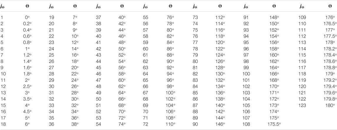
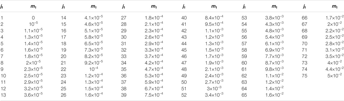
Another decision that affects the number of stored coefficients $\left\{C_p\right\}$ [see Eq. 16] is the choice of a finite set of scattering angles $\text{Θ}$ (angular quadrature). The SIR LUT includes 123 scattering angles $\text{Θ}$ in the range between $0^{\circ }$ and ${180}^{\circ }$ (see Table 1). One may use an appropriate interpolation scheme to estimate the values of aerosol IOPs of interest for the other scattering angles too.

TABLE 1

TABLE 1. Scattering angles $\text{Θ}$ included into the SIR LUT.

We would like to emphasize that the use of this angular quadrature helps to reduce the size of the SIR LUT and optimize its information content. The angular quadrature near scattering angles of $0^{\circ }$ and ${180}^{\circ }$ has ${0.2}^{\circ }$ spacing because the elements of the normalized scattering matrix P [see Eq. 1] can rapidly change there (Hansen and Travis, 1974). The rate of change in P is relatively small between scattering angles of ${10}^{\circ }$ and ${170}^{\circ }$ that allows a coarser angular quadrature with $2^{\circ }$ spacing.

The SK LUT uses an angular quadrature consisting of 181 scattering angles with an equidistant step of $1^{\circ }$ (Dubovik and King, 2000; Dubovik et al., 2002a; Dubovik et al., 2006). This step is too coarse to precisely describe the angular change in the elements of matrix P [see Eq. 1] near scattering angles of $0^{\circ }$ and ${180}^{\circ }$ (Hansen and Travis, 1974).

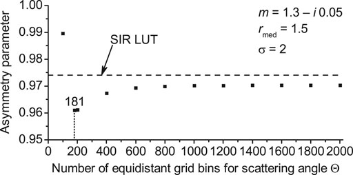
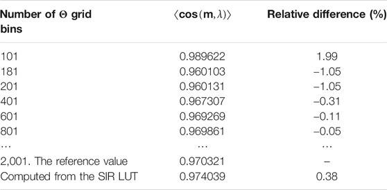
Let us demonstrate the advantage of our angular quadrature with the help of numerical simulations. The asymmetry parameter [see Eq. 6] is a good candidate for a quantitative metric because its computation requires integration over the entire range of scattering angles $\text{Θ}$.

As example input parameters, we select the CRI $m=1.3-i\cdot 0.05$ and a lognormal PSD with $n_{\text{t}}=1{\text{cm}}^{-3}$, $r_{\text{med}}=1.5\mathit{\mu }\text{m}$ and $\sigma =2$ [see Eq. 17]. These parameters are quite unrealistic for ambient aerosols in the visible spectrum (Dubovik et al., 2002b), but we would like to ensure that our “$\pm 1\text{\%}$” requirement is fulfilled across a wide range of scenarios. We selected this particular scenario because it is one of the most difficult cases that we managed to find.

We perform the integration in Eq. 6 using Simpson’s rule on an equidistant grid consisting of 10,001 scattering angles $\text{Θ}$. Out of these 10,001 angles total, the values of phase function are calculated precisely only at a subset of scattering angles, and the rest result from quadratic interpolation. For the tests, we use 101,181 (from $0^{\circ }$ to ${180}^{\circ }$ with the equidistant step of $1^{\circ }$ as in (Dubovik and King, 2000; Dubovik et al., 2002a; Dubovik et al., 2006)), 201, $\dots$, and 2,001 scattering angles. The most precise calculation of the asymmetry parameter is therefore the one integrated using a grid of $\mathrm{2,001}$ scattering angles, and we use this as the reference value. In order to compute the values of the phase function $P_{11}\left(\text{Θ},m,\lambda \right)$ at a wavelength $\lambda =0.355\mathit{\mu }\text{m}$, the Lorenz-Mie computations are made using the Bohren and Huffman code (Bohren and Huffman, 1983). The integration in Eq. 2 is performed for the $2\times {10}^7$ logarithmically equidistant radii bins in the range from ${10}^{-3}$ to $100\mathit{\mu }\text{m}$ (see Section 4.5 for more details).

Figure 2 and Table 2 show the results of the simulations. One can see that the value of the asymmetry parameter computed using 101, 181, and 201 of scattering angles is different by more than $1\text{\%}$ of the reference value. The “$\pm 1\text{\%}$” requirement is fulfilled for the cases of 401 or more scattering angles (see Figure 2 and Table 2). The requirement is also fulfilled by the LUT (see horizontal dashed line at Figure 2 and Table 2). With this we conclude that our quadrature of 123 scattering angles (see Table 1) performs about as well as an equidistant grid consisting of $\mathrm{2,001}$ scattering angles.

FIGURE 2

FIGURE 2. Example asymmetry parameter computation. The vertical dotted line marks the result from the angular quadrature used in the SK LUT.

TABLE 2

TABLE 2. Computed values of the asymmetry parameter.

4.2.3 Quadrature of Complex Refractive Indexes

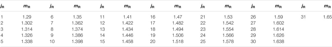
The choice of the CRI quadrature is the last factor which must be chosen to balance the precision of the SIR LUT against the number of stored coefficients $\left\{C_p\right\}$ [see Eq. 16]. Based on our numerical simulations and earlier studies (Dubovik and King, 2000; Dubovik et al., 2002a; Dubovik et al., 2002b; Dubovik et al., 2006), we decided to use $31\cdot 75=\mathrm{2,325}$ CRIs:

• 31 real parts $\left(m_{\text{R}}\right)$ of the CRI in the range between 1.29 and 1.65 with a step 0.012 (see Table 3);

• 75 imaginary parts $\left(m_{\text{I}}\right)$ of the CRI: 0, and 74 logarithmically equidistant values between ${10}^{-5}$ and $5\times {10}^{-2}$ (see Table 4, most of the values are shown rounded).

TABLE 3

TABLE 3. Real parts of the CRI covered by the SIR LUT.

TABLE 4

TABLE 4. Imaginary parts of the CRI covered by the SIR LUT.

Sequential numbers for the real ($j_{\text{R}}$ in Table 3) and imaginary ($j_{\text{I}}$ in Table 4) parts are provided to help navigation inside the SIR LUT file (see Section 4.3).

4.3 Structure of Look-Up Table File

In Section 3 we described the theoretical background of the SIR LUT and in Section 4.2 provided a justification for the selection of quadratures that formed the actual LUT. Starting from this section, we switch our focus on the matters related to the practical application of the SIR LUT.

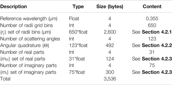
We computed the coefficients $\left\{C_p\right\}$ [see Eq. 16] at a reference wavelength ${\lambda }_{\text{r}}$ and stored them in a file on the computer’s hard drive. The SIR LUT file is binary and consists of a header ($\mathrm{3,536}$ bytes, see Table 5) that is followed by $31\cdot 75=\mathrm{2,325}$ data records ($\mathrm{1,284,408}$ bytes per record, see Table 6) for each CRI separately (see Section 4.2.3). The total size of the file is equal to $\mathrm{3,536}+\mathrm{2,325}\cdot \mathrm{1,284,408}=\mathrm{2,986,252,136}$ bytes. We intentionally limited the size of the SIR LUT file to 3 GB because the majority of modern blade servers have at least 4 GB of RAM per core. The SIR LUT file can then be uploaded into the memory of each core of the blade to further speed up the computations. In the future, we plan to refine the quadratures for the radii and CRIs when the progress in computational hardware will allow us to increase the size of LUT file.

TABLE 5

TABLE 5. Structure of the SIR LUT header.

TABLE 6

TABLE 6. Structure of the SIR LUT data record.

The header contains information defining the reference wavelength and the quadratures for the radii, scattering angles, and CRIs (see Table 5).

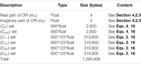
Each data record of the SIR LUT contains the sets of values $\left\{C_p\right\}$ that were computed using Eq. 16 at the reference wavelength ${\lambda }_{\text{r}}=0.355\mathit{\mu }\text{m}$ (see Table 6). For the computations we used a reliable and accurate Lorenz-Mie scattering program (Mishchenko et al., 2002; Mishchenko, 2019). We slightly modified the program to make it suitable for parallel computation of the coefficients $C_{p,j,{\lambda }_{\text{r}}}$ [see Eq. 16], but the core part of the program remained intact. We used $\mathrm{100,000}$ points over each integration range of radii $\left[r_j,r_{j+1}\right]$ by setting the program input parameters N = $\mathrm{1,000}$ (number of subintervals within $\left[r_j,r_{j+1}\right]$) and NK = 100 (number of Gaussian division points) (Mishchenko et al., 2002; Mishchenko, 2019). All the SIR LUT related computations were performed on blade servers equipped with Intel Xeon “Skylake” processors on the NASA LaRC K-Cluster.

The $\left\{C_{11}\right\}$, $\left\{C_{12}\right\}$, $\left\{C_{33}\right\}$, and $\left\{C_{34}\right\}$ sets in Table 6 are two dimensional arrays that are stored line by line, i.e., 650 lines (corresponding to the radii quadrature, see Section 4.2.1) with 123 columns each (corresponding to the scattering angles quadrature, see Section 4.2.2).

The beginning position in the SIR LUT file for the data record that corresponds to a certain CRI can be computed using the sequential numbers of the real and imaginary parts (see Section 4.2.3) as $\mathrm{3,536}+\mathrm{1,284,408}\cdot \left(75\cdot \left(j_{\text{R}}-1\right)+j_{\text{I}}-1\right)$ bytes. For instance, if one needs the data record that corresponds to the CRI with real part $m_{\text{R}}=1.362$ ($j_{\text{R}}=7$) and imaginary part $m_{\text{I}}=2.6\times {10}^{-4}$ ($j_{\text{I}}=30$) then the pointer inside of the SIR LUT file should be set at the position of $\mathrm{615,234,968}$ bytes from the beginning of file.

We also share with the community codes written in C++, Fortran, Python and Matlab that can be used to efficiently compute all aerosol IOPs of interest [see Eqs. 2–6] from the SIR LUT.

4.4 Usage of Look-Up Table

To make the practical use of the SIR LUT, it is necessary to develop a way of computing the coefficients $C_{p,j,\lambda }$ at longer wavelengths λ using coefficients $C_{p,j,{\lambda }_{\text{r}}}$ precomputed at the reference wavelength ${\lambda }_{\text{r}}$. At this point, we have already decided on reference wavelength and quadratures that define the structure of the SIR LUT and highlighted the useful properties of efficiencies by applying the scale invariance rule (Mishchenko, 2006). We return to theoretical derivations one last time to complete the final assembly by collecting these fragments into a working mechanism.

As discussed in Section 4.1, since it is the size parameter that drives the single-scattering computations, the integration of efficiencies at longer wavelengths can be directly expressed through the integration of efficiencies calculated at a shorter wavelength. Equation 21 allows us to apply a linear scaling of the quadratic approximation range [see Eq. 12] from $\left[r_{j-1},r_{j+1}\right]$ to $\left[\frac{{\lambda }_{\text{r}}}{\lambda }{r}_{j-1},\frac{{\lambda }_{\text{r}}}{\lambda }{r}_{j+1}\right]$ in order to switch in Eq. 16 from an arbitrary wavelength $\lambda \mathrm{\ge }{\lambda }_{\text{r}}$ to the reference wavelength ${\lambda }_{\text{r}}$. After repeating the PSD quadratic approximation procedure [see Eqs. 12–16], the coefficient $C_{p,j,\lambda }$ in Eq. 16 can be computed as

$\frac{{\lambda }_{\text{r}}}{\lambda }\left[\begin{array}{l}\frac{3\ln \frac{{\lambda }_{\text{r}}}{\lambda }{r}_{j-2}\ln \frac{{\lambda }_{\text{r}}}{\lambda }{r}_{j-1}}{8{\left(\text{Δ}\ln r\right)}^2}{\displaystyle {\int }_{\frac{{\lambda }_{\text{r}}}{\lambda }{r}_{j-1}}^{\frac{{\lambda }_{\text{r}}}{\lambda }{r}_j}\frac{Q_p\left(\cdot ,r,{\lambda }_{\text{r}}\right)}{r}\text{d}\ln r}\\ -\frac{3\ln \frac{{\lambda }_{\text{r}}^2}{{\lambda }^2}{r}_{j-2}{r}_{j-1}}{8{\left(\text{Δ}\ln r\right)}^2}{\displaystyle {\int }_{\frac{{\lambda }_{\text{r}}}{\lambda }{r}_{j-1}}^{\frac{{\lambda }_{\text{r}}}{\lambda }{r}_j}\ln r\frac{Q_p\left(\cdot ,r,{\lambda }_{\text{r}}\right)}{r}\text{d}\ln r}\\ +\frac{3}{8{\left(\text{Δ}\ln r\right)}^2}{\displaystyle {\int }_{\frac{{\lambda }_{\text{r}}}{\lambda }{r}_{j-1}}^{\frac{{\lambda }_{\text{r}}}{\lambda }{r}_j}{\ln }^{2}r\frac{Q_p\left(\cdot ,r,{\lambda }_{\text{r}}\right)}{r}\text{d}\ln r}\\ -\frac{3\ln \frac{{\lambda }_{\text{r}}}{\lambda }{r}_{j-1}\ln \frac{{\lambda }_{\text{r}}}{\lambda }{r}_{j+1}}{4{\left(\text{Δ}\ln r\right)}^2}{\displaystyle {\int }_{\frac{{\lambda }_{\text{r}}}{\lambda }{r}_j}^{\frac{{\lambda }_{\text{r}}}{\lambda }{r}_{j+1}}\frac{Q_p\left(\cdot ,r,{\lambda }_{\text{r}}\right)}{r}\text{d}\ln r}\\ +\frac{3\text{ln}\frac{{\lambda }_{\text{r}}^2}{{\lambda }^2}{r}_{j-1}{r}_{j+1}}{4{\left(\text{Δ}\text{ln}r\right)}^2}{\displaystyle {\int }_{\frac{{\lambda }_{\text{r}}}{\lambda }{r}_j}^{\frac{{\lambda }_{\text{r}}}{\lambda }{r}_{j+1}}\ln r\frac{Q_p\left(\cdot ,r,{\lambda }_{\text{r}}\right)}{r}\text{d}\ln r}\\ -\frac{3}{4{\left(\text{Δ}\ln r\right)}^2}{\displaystyle {\int }_{\frac{{\lambda }_{\text{r}}}{\lambda }{r}_j}^{\frac{{\lambda }_{\text{r}}}{\lambda }{r}_{j+1}}{\ln }^{2}r\frac{Q_p\left(\cdot ,r,{\lambda }_{\text{r}}\right)}{r}\text{d}\ln r}\\ +\frac{3\ln \frac{{\lambda }_{\text{r}}}{\lambda }{r}_{j+1}\ln \frac{{\lambda }_{\text{r}}}{\lambda }{r}_{j+2}}{8{\left(\text{Δ}\ln r\right)}^2}{\displaystyle {\int }_{\frac{{\lambda }_{\text{r}}}{\lambda }{r}_{j+1}}^{\frac{{\lambda }_{\text{r}}}{\lambda }{r}_{j+2}}\frac{Q_p\left(\cdot ,r,{\lambda }_{\text{r}}\right)}{r}\text{d}\ln r}\\ -\frac{3\ln \frac{{\lambda }_{\text{r}}^2}{{\lambda }^2}{r}_{j+1}{r}_{j+2}}{8{\left(\text{Δ}\ln r\right)}^2}{\displaystyle {\int }_{\frac{{\lambda }_{\text{r}}}{\lambda }{r}_{j+1}}^{\frac{{\lambda }_{\text{r}}}{\lambda }{r}_{j+2}}\ln r\frac{Q_p\left(\cdot ,r,{\lambda }_{\text{r}}\right)}{r}\text{d}\ln r}\\ +\frac{3}{8{\left(\text{Δ}\ln r\right)}^2}{\displaystyle {\int }_{\frac{{\lambda }_{\text{r}}}{\lambda }{r}_{j+1}}^{\frac{{\lambda }_{\text{r}}}{\lambda }{r}_{j+2}}{\ln }^{2}r\frac{Q_p\left(\cdot ,r,{\lambda }_{\text{r}}\right)}{r}\text{d}\ln r}\end{array}\right]\cdot (24)$

The common multiplier $\frac{{\lambda }_{\text{r}}}{\lambda }$ in front of the bracket appears in Eq. 24 to compensate the division by radius r during each integration. If desired, one can verify the equivalence of Eqs. 16 and 24 numerically or prove it analytically using Eq. 22.

In practice, it is necessary to use an interpolation technique to estimate the coefficient $C_{p,j,\lambda }$ because in the general case the scaled radius $\frac{{\lambda }_{\text{r}}}{\lambda }{r}_j$ does not coincide with any of the SIR LUT radius quadrature points $\left\{r_j\right\}$ (see Sections 3 and 4.2.1). As an option, quadratic interpolation may be used with the known LUT values of coefficient at radius quadrature points $r_{k-1}$, $r_k$, and $r_{k+1}$:

$C_{p,j,\lambda }\approx \frac{{\lambda }_{\text{r}}}{\lambda }\left[\begin{array}{l}{C}_{p,k-1,{\lambda }_{\text{r}}}\frac{\left(\frac{{\lambda }_{\text{r}}}{\lambda }{r}_j-r_k\right)\left(\frac{{\lambda }_{\text{r}}}{\lambda }{r}_j-r_{k+1}\right)}{\left(r_{k-1}-r_k\right)\left(r_{k-1}-r_{k+1}\right)}\\ +C_{p,k,{\lambda }_{\text{r}}}\frac{\left(\frac{{\lambda }_{\text{r}}}{\lambda }{r}_j-r_{k-1}\right)\left(\frac{{\lambda }_{\text{r}}}{\lambda }{r}_j-r_{k+1}\right)}{\left(r_k-r_{k-1}\right)\left(r_k-r_{k+1}\right)}\\ +C_{p,k+1,{\lambda }_{\text{r}}}\frac{\left(\frac{{\lambda }_{\text{r}}}{\lambda }{r}_j-r_{k-1}\right)\left(\frac{{\lambda }_{\text{r}}}{\lambda }{r}_j-r_k\right)}{\left(r_{k+1}-r_{k-1}\right)\left(r_{k+1}-r_k\right)}\end{array}\right],(25)$

where the index k is generally selected to fulfill $r_k\mathrm{\le }\frac{{\lambda }_{\text{r}}}{\lambda }{r}_j\mathrm{\le }{r}_{k+1}$ when the quadrature point $r_{k-1}$ is available for the case $\lambda \mathrm{\ge }{\lambda }_{\text{r}}$ and the quadrature point $r_{k+1}$ can go up to $r_{\text{max}}=100\mu$m. If the index k is found to be equal to unity then the coefficient $C_{p,j,\lambda }$ is computed using Eq. 25 at the radius quadrature points $r_1$, $r_2$, and $r_3$. If the scaled radius $\frac{{\lambda }_{\text{r}}}{\lambda }{r}_j$ is too small and not covered by the SIR LUT at all (see discussion related to the increase of $r_{\text{min},\lambda }$ in Section 4.2.1) then the coefficient $C_{p,j,\lambda }$ vanishes. As the wavelength of interest λ increases, the contribution from the smallest particles is lost with the relatively minor impact.

Different interpolation techniques, instead of quadratic as in Eq. 25, also may be applied. One should keep in mind that quadratic interpolation provides reasonable results and requires only nine multiplications and three divisions that can be done quite fast considering that 650 interpolations are needed for each aerosol IOP p [see Eq. 11].

Equation 25 offers a simple way to compute the coefficients $C_{p,j,\lambda }$ at longer wavelengths using the precomputed and stored coefficients $C_{p,j,{\lambda }_{\text{r}}}$. One may skip all the mathematical theory behind Eq. 25 as it might look complicated. In the end, the elegance of this LUT approach allows us to exchange the integration in Eqs. 2–4 at longer wavelengths with an integration at a shorter reference wavelength over a range of smaller radii.

4.5 Validation of the Scale Invariance Rule Look-Up Table: Unit Tests

To demonstrate the improved capabilities of the SIR LUT, we will compute the aerosol IOPs of interest [see Eqs. 2–6] using the SIR LUT [see Eqs. 11, 25] and compare them to simulated truth values (see Section 4.5.1).

At the beginning we set a $\pm 1\text{\%}$ relative difference for all single-scattering properties [see Eqs. 2–6] as the precision target. The $\pm 1\text{\%}$ precision shall be achieved at all the wavelengths of interest, i.e., at $\left\{\lambda \right\}=\left\{0.355,0.41,0.469,0.532,0.555,0.67,0.864,0.96,1.064,1.594,1.88,2.264\right\}\mathit{\mu }\text{m}$ (see Section 1). In Section 4.1 we anticipated that the targeted precision would be most difficult to achieve at the shortest wavelength, i.e. at $\lambda =0.355\mathit{\mu }\text{m}$, despite the fact that it is the reference wavelength.

We compute the relative difference for the aerosol IOPs $p=\left\{\beta \left(m,\lambda \right),\text{sca}\left(m,\lambda \right),\alpha \left(m,\lambda \right),\text{abs}\left(m,\lambda \right),\langle \text{cos}\left(m,\lambda \right)\rangle \right\}$ [see Eqs. 3–6] as

${\delta }_p=\frac{p-p_{\text{t}}}{p_{\text{t}}}\cdot 100\text{\%},(26)$

where $p_{\text{t}}$ is the simulated truth value for the aerosol IOP p.

For the elements of the normalized scattering matrix P [see Eq. 2] the relative difference is computed slightly differently:

${\delta }_{P_{ii\prime }}\left(\text{Θ}\right)=\frac{P_{ii\prime }\left(\text{Θ}\right)-P_{ii\prime ,\text{t}}\left(\text{Θ}\right)}{\underset{\text{Θ}}{\text{max}}\left|P_{ii\prime ,\text{t}}\left(\text{Θ}\right)\right|}\cdot 100\text{\%},(27)$

where $P_{ii\prime ,\text{t}}\left(\text{Θ}\right)$ is the simulated truth of the normalized scattering matrix element $P_{ii\prime }\left(\text{Θ}\right)$. We compare the difference between the SIR LUT and the simulated truth values with the maximum absolute simulated truth value because at some scattering angles $\text{Θ}$ the value of $P_{ii\prime ,\text{t}}\left(\text{Θ}\right)$ element may be close to zero or vanish for natural reasons. It is important to reproduce the shape of $P_{ii\prime ,\text{t}}\left(\text{Θ}\right)$ functions around their peaks, which for aerosols mainly occur at scattering angles $\text{Θ}$ close to $0^{\circ }$ and ${180}^{\circ }$ (see Section 4.2.2). By contrast, a $1\text{\%}$ disagreement when the absolute value of the element is small tends to be more acceptable for our purposes of modeling lidar and polarimeter observables.

4.5.1 Simulated Truth

It is now time to clarify the aerosol IOPs $\left\{p_{\text{t}},P_{ii\prime ,\text{t}}\left(\text{Θ}\right)\right\}$ that we consider to be the simulated truth for comparisons in the unit tests. To compute the true IOPs $\left\{p_{\text{t}},P_{ii\prime ,\text{t}}\left(\text{Θ}\right)\right\}$, we have to decide which CRIs, PSDs, and scattering angles $\text{Θ}$, as well as the integration range $\left[r_{\text{min}},r_{\text{max}}\right]$ and integration settings to use in Eqs. 2–6.

During retrievals of aerosol microphysical properties using real lidar and polarimeter data, the values of the CRIs will not necessarily coincide with the CRI quadrature of the SIR LUT (see Section 4.2.3). A two-dimensional interpolation scheme is used to obtain the off-CRI-grid values of aerosol IOPs $\left\{p,P_{ii\prime }\left(\text{Θ}\right)\right\}$ using several values of the same IOP estimated using the LUT at CRI grid points. We recommend the use of quadratic interpolation [see Eq. 25] in two dimensions since we found it to be fast and reliable.

In the unit tests we shall focus on the off-grid CRIs that are covered but not directly included into the SIR LUT (see Section 4.2.3) and that are realistic from the perspective of ambient aerosols (Dubovik et al., 2002b). Keeping this in mind, we selected to use the set consisting of $18\cdot 101=\mathrm{1,818}$ CRIs: 18 real parts $\left(m_{\text{R}}\right)$ of the CRI in the range between 1.31 and 1.65 with a step of 0.02, and 101 imaginary parts $\left(m_{\text{I}}\right)$ of the CRI consisting of 0, and 100 equidistant values between $2.5\times {10}^{-4}$ and 0.04975 with a step of $5\times {10}^{-4}$. Among these $\mathrm{1,818}$ CRIs there are six that form a subset $\left\{\text{m}\right\}=\left\{1.35,1.41,1.47,1.53,1.59,1.65\right\}$ that intersects with the CRI quadrature of the SIR LUT (see Section 4.2.3). It is reasonable to expect high precision of the SIR LUT at CRIs $\in \left\{\text{m}\right\}$. We will use this property of the $\left\{\text{m}\right\}$ subset as an additional benchmark test to help evaluate the quality of our unit tests.

Let us use a monomodal lognormal distribution (see Section 3.1) as the function $n\left(r\right)$ in Eqs. 2–6 to simulate an ambient aerosol PSD (Kolmogorov, 1941; Seinfeld and Pandis, 2006). The count median radius $r_{\text{med}}$ [see Eq. 18] in our unit tests will vary from 0.075 to $1.501\mathit{\mu }\text{m}$ with a constant step of $0.002\mathit{\mu }\text{m}$ (for a total of 714 values). Twelve geometric standard deviations σ [see Eq. 18] in the range from 1.35 to 2.01 with a constant step of 0.06 will accompany each median radius. It is enough to consider a single total number concentration $n_{\text{t}}=1{\text{cm}}^{-3}$ [see Eq. 18] to evaluate relative differences in the single-scattering properties. These $714\cdot 12=\mathrm{8,568}$ PSDs cover a wide range of aerosol size distributions (Dubovik et al., 2002b).

Thus, the total number of CRI–PSD unit tests is equal to $\mathrm{1,818}\cdot \mathrm{8,568}=\mathrm{15,576,624}$ at each wavelength of interest $\left\{\lambda \right\}$.

Recall from Section 4.2.2, the SIR LUT uses a quadrature of 123 scattering angles that precisely represents the aerosol asymmetry parameter as well as equidistant quadratures with many more angles. Therefore, we use this scattering angle quadrature in our unit test dataset as well. Let us compute the simulated truth elements $P_{ii\prime ,\text{t}}\left(\text{Θ}\right)$ of normalized scattering matrices [see Eq. 1] for the same angular quadrature.

Putting it all together, we track $5+4\cdot 123=497$ relative differences [see Eqs. 26, 27] of aerosol IOPs [see Eqs. 2–6] with a $\pm 1\text{\%}$ precision target.

For all wavelengths of interest let us compute the simulated truth $\left\{p_{\text{t}},P_{ii\prime ,\text{t}}\left(\text{Θ}\right)\right\}$ by integrating over the radius range $\left[r_{\text{min}}=0.001\mu \text{m},r_{\text{max}}=100\mu \text{m}\right]$ that the SIR LUT uses at a wavelength of $0.355\mathit{\mu }\text{m}$ (see Section 4.2.1). This radius integration range covers the majority of ambient fine and coarse mode aerosol PSDs (Dubovik et al., 2002b). With nanoparticles included into integration at all wavelengths, we can evaluate the losses of information about nanoparticles by the SIR LUT with the increase of wavelength (see discussion related to the increase of $r_{\text{min},\lambda }$ in Section 4.2.1).

The only remaining decision is how many radius quadrature points are used if Simpson’s rule is applied to the numerical integration in Eqs. 2–6. The absorption coefficient at $\lambda =0.355\mathit{\mu }\text{m}$ is an IOP that can help us make this decision. In Section 4.2.1 we selected the CRI $m=1.65-i\cdot {10}^{-5}$ as an example where the absorption efficiency oscillates with an amplitude exceeding two orders of magnitude (see Figure 1, solid curve). Such highly oscillatory functions require a very narrow integration step to produce a precise result. For such cases, if we increase the number of logarithmically equidistant radii bins by factor of ten, we expect the computed absorption coefficient to converge and the relative difference to decrease and approach zero. We set the parameters of the aerosol PSD to $n_{\text{t}}=1{\text{cm}}^{-3}$, $r_{\text{med}}=0.7\mathit{\mu }\text{m}$ and $\sigma =1.35$ [see Eq. 18].

To compute the simulated truth values, the Lorenz-Mie single-scattering calculations were performed using the well-established Bohren and Huffman program (Bohren and Huffman, 1983). As a reminder, the SIR LUT coefficients (see Section 4.3) were computed using the Mishchenko et al. program (Mishchenko et al., 2002; Mishchenko, 2019). By cross-checking the two Lorenz-Mie programs we achieved a high level of confidence in the unit tests.

4.5.2 Results of the Unit Tests

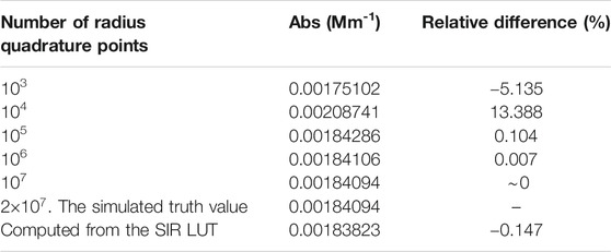
Table 7 lists the results of the numerical integration. As the number of radius quadrature points increases, the value of the absorption coefficient converges, as expected. After the number of points reaches ${10}^5$, the $\pm 1\text{\%}$ precision level is achieved, but even more points are needed to converge to the value that would be considered the simulated truth. The relative difference between the ${10}^7$ and $2\times {10}^7$ radius quadrature points is close to numerical zero, which is the best we can expect in terms of convergence.

TABLE 7

TABLE 7. Computed values of the aerosol absorption coefficient.

The absolute value of the absorption coefficient in this test is small because the imaginary part of CRI is very close to zero. We intentionally selected this almost non-absorbing aerosol because during the SIR LUT development stage we experienced the most difficulties in achieving $\pm 1\text{\%}$ precision for the low absorbing particles.

Based on Table 7, we made a decision to compute all the simulated truth aerosol IOPs $\left\{p_{\text{t}},P_{ii\prime ,\text{t}}\left(\text{Θ}\right)\right\}$ [see Eqs. 2–6] by applying Simpson’s rule using $2\times {10}^7$ logarithmically equidistant radius quadrature points in the range from ${10}^{-3}$ to $100\mathit{\mu }\text{m}$. We may have to use even more quadrature points if, in the future, the SIR LUT is extended to have more imaginary parts of the CRI between 0 and ${10}^{-5}$. One can see that solid curve in Figure 1 has multiple spikes at least two orders of magnitude from the basic trend. For imaginary parts below ${10}^{-5}$ we expect to see efficiencies that are even more oscillatory compared to the solid curve of Figure 1.

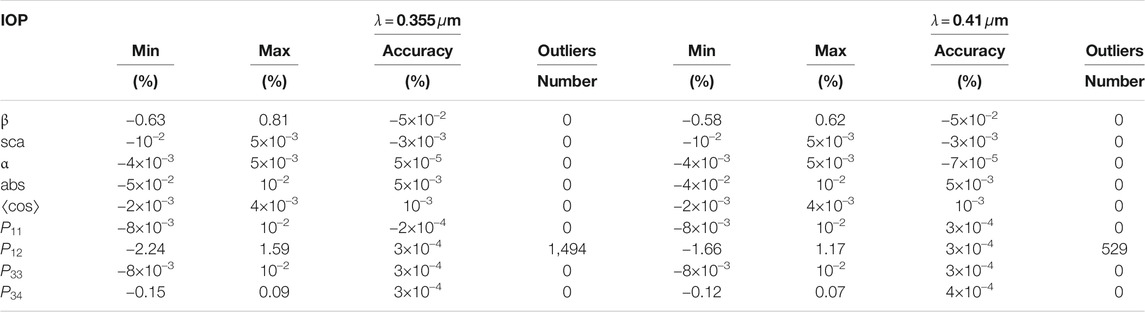
Moving further, we computed the simulated truth values for all the aerosol IOPs [see Eqs. 2–6] at twelve wavelengths $\left\{\lambda \right\}$ and compared them [see Eqs. 26, 27] to the corresponding LUT values [see Eqs. 11, 25]. The targeted $\pm 1\text{\%}$ precision level was achieved in all cases except for the $P_{12}\left(\text{Θ}\right)$ element of the normalized scattering matrix, which turned out to be the most difficult aerosol IOP to tabulate. All the other aerosol IOPs were computed using the SIR LUT within the targeted precision.

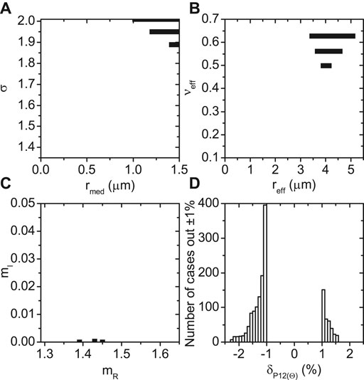
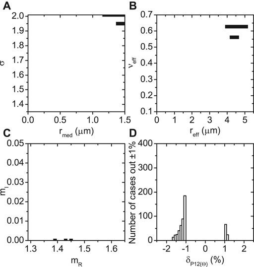
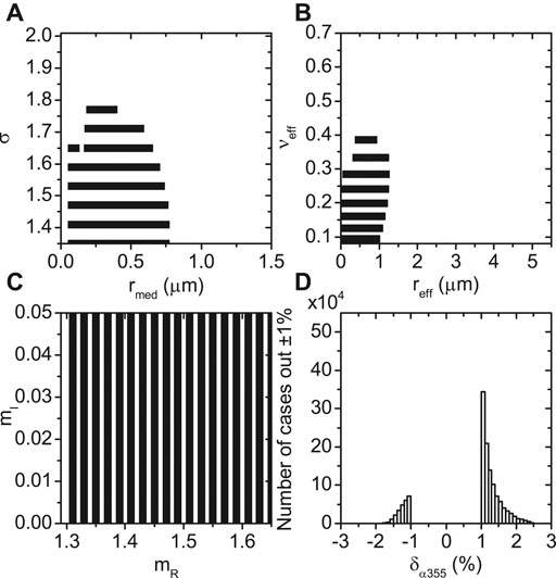
Figures 3, 4 and Table 8 show the details of the CRI–PSD unit tests at two minimum wavelengths of interest that lead to a relative error [see Eq. 27] larger than $\pm 1\text{\%}$ for the element $P_{12}\left(\text{Θ}\right)$. Panels (A) and (B) of Figures 3, 4 detail the locations of the problematic PSDs in terms of median radius and geometric standard deviation (A), and effective radius and effective variance (B). Panel (C) of Figures 3, 4 depicts the locations of problematic CRIs, and panel (D) provides the histograms of relative differences for only the unit tests that failed to reach the $1\text{\%}$ precision.

FIGURE 3

FIGURE 3. Outliers in $P_{12}\left(\text{Θ}\right)$ computations from the SIR LUT at $\lambda =0.355\mu \text{m}$. Description of labels is given in text.

FIGURE 4

FIGURE 4. Outliers in $P_{12}\left(\text{Θ}\right)$ computations from the SIR LUT at $\lambda =0.41\mu \text{m}$. Description of labels is given in text.

TABLE 8

TABLE 8. Overview of the SIR LUT performance.

One can see that the problematic PSDs describe coarse mode aerosols with an effective radius exceeding $3.5\mathit{\mu }\text{m}$ and an effective variance exceeding 0.45 (see panel (B) of Figures 3, 4). These effective radii and variances correspond to large aerosols with sizes that are sparsely covered by our logarithmically equidistant distributed set $\left\{r_j\right\}$ of radius quadrature points (see Sections 3 and 4.2.1). All the problematic CRIs have an imaginary part around zero (see panel (C) of Figures 3, 4). We thus expect that the $Q_{12}\left(\text{Θ},m,\lambda =0.355\mu m,r\right)$ directional scattering efficiency for small imaginary parts oscillates even more vigorously than the absorption efficiency (see solid curve of Figure 1). If we find it necessary to improve the precision of $P_{12}\left(\text{Θ}\right)$, in the next version of the SIR LUT we will need to have more radius quadrature points M (see Section 4.2.1), denser coverage of imaginary parts of CRI around zero (see Section 4.2.3), and possibly use additional integration points to compute the values of simulated truth and the SIR LUT coefficients [see Eq. 16]. The current version of the SIR LUT allows us to estimate the $P_{12}\left(\text{Θ}\right)$ element of the normalized scattering matrix to within $\pm 2.5\text{\%}$ (see panel (D) of Figures 3, 4 and Table 8).

Let us point out that panel (C) of Figures 3, 4 is missing the points corresponding to the subset $\left\{\text{m}\right\}$ mentioned earlier. Interestingly, the CRI point $\left(1.41,0\right)\in \left\{\text{m}\right\}$ is absent from panel (C) but two of its closest neighbors $\left(1.39,0\right)\notin \left\{\text{m}\right\}$ and $\left(1.43,0\right)\notin \left\{\text{m}\right\}$ are marked as the problematic CRIs. Intuition suggests that the CRI point between those two also has a potential to be problematic. We expect to have the highest precision of the SIR LUT at the points of the CRI quadrature and one of them is the point $\left(1.41,0\right)\in \left\{\text{m}\right\}$, which explains its absence from panel (C). We consider this feature to be an additional indicator of proper behavior by the SIR LUT.

Panel (D) of Figures 3, 4 show the histograms of $P_{12}\left(\text{Θ}\right)$ relative differences [see Eq. 27] for the problematic CRI–PSD unit tests out of $\mathrm{15,576,624}$ total tests spanning the entire scattering angle quadrature consisting of 123 angles (see Section 4.2.2). The $\pm 1\text{\%}$ precision target was not achieved $\mathrm{1,494}$ times at a wavelength of $0.355\mathit{\mu }\text{m}$ ($7.8\times {10}^{-5}\text{\%}$; see Figure 3D and Table 8) and 529 times at $0.41\mathit{\mu }\text{m}$ ($2.8\times {10}^{-5}\text{\%}$; see Figure 4D and Table 8). In Section 4.1 we anticipated improvement in the SIR LUT precision as the wavelength increases and Figures 3, 4 together with Table 8 confirm this behavior. The trend of a reduction in the number of problematic cases continues as the wavelength increases and the number drops to zero at $0.532\mathit{\mu }\text{m}$.

To increase confidence in the precision of the SIR LUT, we conducted an additional test using $\mathrm{1,000,000}$ random λ–CRI–PSD unit tests. A uniform random number generator provided evenly distributed values of wavelength λ in the range from 0.355 to $2.264\mathit{\mu }\text{m}$, count median radius $r_{\text{med}}$ from 0.075 to $1.5\mathit{\mu }\text{m}$, geometric standard deviation σ from 1.35 to 2.01, real part of the CRI $m_{\text{R}}$ from 1.31 to 1.65, and imaginary part of the CRI $m_{\text{I}}$ from 0 to 0.05. Using these random inputs, we computed the simulated truth values for all the aerosol IOPs [see Eqs. 2–6] and compared them to the corresponding SIR LUT values [see Eqs. 11, 25]. The $\pm 1\text{\%}$ precision was not achieved in eleven cases for the aerosol absorption coefficient and once for the $P_{12}\left(\text{Θ}\right)$ element of the normalized scattering matrix. All these cases have an imaginary part of the CRI between 0 and ${10}^{-5}$. Qualitatively, the assessment is very similar to what is shown in Figures 3, 4.

With the presented results of numerical simulations, we conclude that the performance of the SIR LUT for all the aerosol IOPs of interest is precise to within $\pm 1\text{\%}$ except for a few cases where $P_{12}\left(\text{Θ}\right)$ is within $\pm 2.5\text{\%}$. The impact of the precision of $P_{12}\left(\text{Θ}\right)$ on polarimeter observables will be explored in Section 4.7.

4.6 Validation of the Spherical Kernels Look-Up Table: Unit Tests

An important topic to consider is the precision of the SK LUT that is currently in use and served as the inspiration for the SIR LUT (Dubovik and King, 2000; Dubovik et al., 2002a; Dubovik et al., 2006). It is first necessary to understand what improvements, if any, are achieved using quadratic approximation of the aerosol PSD [see Eq. 12] and by the cost of increasing the number of stored coefficients (see Sections 4.2–4.3). We will also provide more details on the aerosol lidar backscatter and extinction coefficients. For the other aerosol IOPs we provide histograms with relative differences. It is sufficient to explore only the 0.355 and $0.532\mathit{\mu }\text{m}$ wavelengths to study if the precision of the SK LUT also improves as the wavelength increases. For brevity, we skip the wavelength of $1.064\mathit{\mu }\text{m}$ that is also used by the HSRL-2 instrument. The relative difference comparisons are made using the same simulated truth values for the $\mathrm{15,576,624}$ unit tests that are described in Section 4.5.

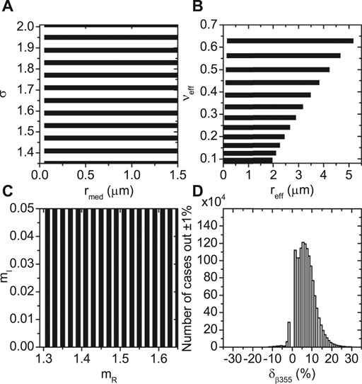
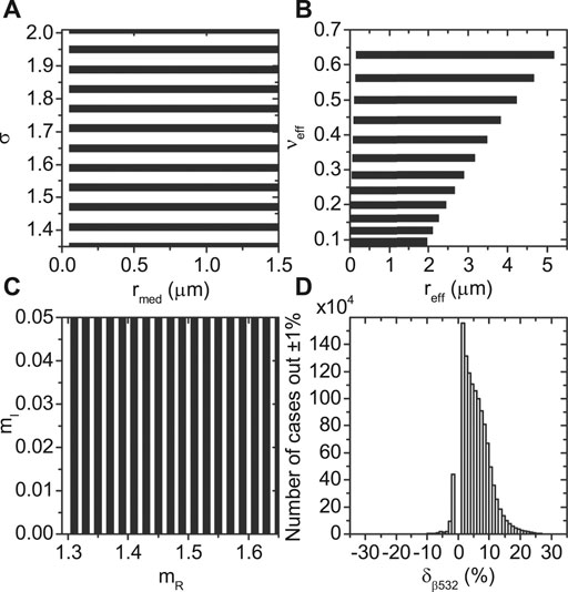
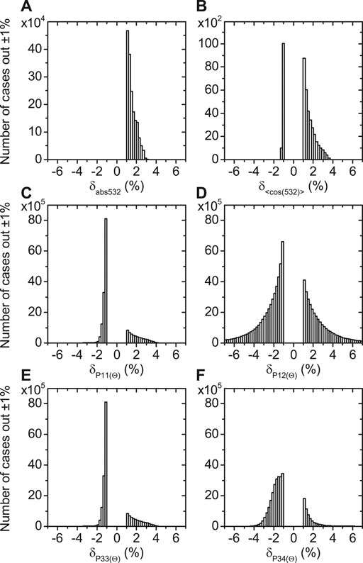
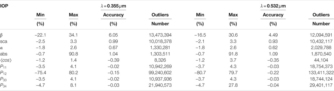
Figures 5–10 and Table 9 show the results of comparisons. Each dot in the panels (A–C) of Figures 5–8 indicates that $\pm 1\text{\%}$ relative difference was not achieved for at least one HSRL-2 UV–VIS observable for a given CRI or PSD. The histograms in panel (D) of Figures 5–8 and all panels of Figures 9, 10 plot the distribution of relative differences [see Eqs. 26, 27] that are greater than $\pm 1\text{\%}$.

FIGURE 5

FIGURE 5. Outliers in ${\beta }_{355}$ computations from the SK LUT. Description of labels is given in text.

FIGURE 6

FIGURE 6. Outliers in ${\alpha }_{355}$ computations from the SK LUT. Description of labels is given in text.

FIGURE 7

FIGURE 7. Outliers in ${\beta }_{532}$ computations from the SK LUT. Description of labels is given in text.

FIGURE 8

FIGURE 8. Outliers in ${\alpha }_{532}$ computations from the SK LUT. Description of labels is given in text.

FIGURE 9

FIGURE 9. Overview of the SK LUT outliers at $\lambda =0.355\mu \text{m}$. Description of labels is given in text.

FIGURE 10

FIGURE 10. Overview of the SK LUT outliers at $\lambda =0.532\mu \text{m}$. Description of labels is given in text.

TABLE 9

TABLE 9. Overview of the SK LUT performance.

In this test of the SK LUT, we found that the backscatter coefficient at $0.355\mathit{\mu }\text{m}$ had the worst accuracy and precision (see Figure 5 and Table 9). The $\pm 1\text{\%}$ relative difference was not achieved $\mathrm{13,473,394}$ times at a wavelength of $0.355\mathit{\mu }\text{m}$ ($86.5\text{\%}$) and $\mathrm{12,094,591}$ times at $0.532\mathit{\mu }\text{m}$ ($77.65\text{\%}$). The relative differences of HSRL-2 UV–VIS observables are within $\pm 35\text{\%}$ at $0.355\mathit{\mu }\text{m}$ (see Figure 5D and Table 9) and $\pm 31\text{\%}$ at $0.532\mathit{\mu }\text{m}$ (see Figure 7D and Table 9). The relative difference also improves as the wavelength increases as we anticipated in Section 4.1 for this type of LUT, and which we have already seen for the SIR LUT in Section 4.5. The improvement is relatively minor and every CRI and PSD was found to result in a computed lidar backscatter coefficient with a relative difference of greater than $\pm 1\text{\%}$ at least once (see panels (A–C) of Figures 5, 7).

All four relative difference histograms (see panel (D) of Figures 5–8) of the HSRL-2 UV–VIS observables are asymmetric, and indicate a tendency of the SK LUT to overestimate the HSRL-2 observables. It is unexpected to see an overestimation here, because of the significant difference in the integration range for radius. We computed the simulated truth values with the integration range up to $r_{\text{max}}=100\mathit{\mu }\text{m}$ [see Eqs. 3, 4]. By contrast, the SK LUT stops at $\sim 33.9\mathit{\mu }\text{m}$ in terms of particle radius (Dubovik and King, 2000; Dubovik et al., 2002a; Dubovik et al., 2006). The information between $\sim 33.9$ and $100\mathit{\mu }\text{m}$ is lost, and that naturally should lead to underestimations. The reason for systematic overestimates is unknown but will be investigated separately.

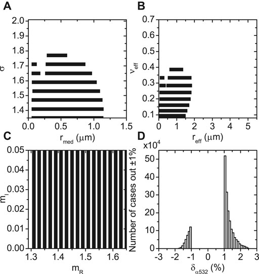
Compared to the lidar backscatter coefficient, the accuracy and precision of the extinction coefficient are noticeably better (see Figures 6, 8 and Table 9). The $\pm 1\text{\%}$ relative difference was not achieved $\mathrm{1,330,281}$ times at a wavelength of $0.355\mathit{\mu }\text{m}$ ($8.54\text{\%}$) and $\mathrm{2,029,788}$ times at $0.532\mathit{\mu }\text{m}$ ($13.03\text{\%}$). The relative differences are within $\pm 3\text{\%}$ at both 0.355 (see Figure 6D and Table 9) and $0.532\mathit{\mu }\text{m}$ (see Figure 8D and Table 9). It is unexpected to see that the SK LUT precision for the extinction coefficient degrades with the increase of wavelength, but the interesting feature is that degradation appears to be approximately proportional to the scaling factor $\frac{0.532}{0.355}\approx 1.5$. The same scaling factor of $\sim 1.5$ can be noticed in terms of the effective radius too. The estimations with SK LUT show precision issues for PSDs with effective radius up to $1.2\mathit{\mu }\text{m}$ at wavelength $0.355\mathit{\mu }\text{m}$ and up to $1.8\mathit{\mu }\text{m}$ at $0.532\mathit{\mu }\text{m}$ (see panel (B) of Figures 6, 8). Most probably, this decrease in precision happens because of features specific to the extinction efficiencies that are amplified by the fact that the SK LUT has only 41 radius quadrature points (Dubovik and King, 2000; Dubovik et al., 2002a; Dubovik et al., 2006) compared to 650 for the SIR LUT (see Section 4.2.1). It is known that extinction efficiencies are the most oscillatory for the values of the size parameter $x\ge 10$ (Van de Hulst, 1981; Bohren and Huffman, 1983; Mishchenko et al., 2002). As the size parameter increases, the extinction efficiencies asymptotically approach a constant value. As a result, it is sufficient to use fewer radius quadrature points to characterize the extinction efficiency function for PSDs of larger particles; this leads to more precise extinction coefficients for coarse mode aerosols by the SK LUT.

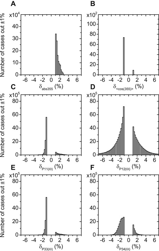
The accuracy and precision of the SK LUT for the absorption coefficient (see panel (A) of Figures 9, 10 and Table 9) and all the four elements of the normalized scattering matrix (see panels (C–F) of Figures 9, 10 and Table 9) also degrade as the wavelength increases. Only the $P_{12}\left(\text{Θ}\right)$ element has a fairly symmetric histogram of relative differences (see panel (D) of Figures 9, 10). Panels (C–F) of Figures 9, 10 and Table 9 reflect the results of comparisons that were done only at 101 scattering angles which are common between the angular quadratures of the SIR LUT (see Section 4.2.2) and the SK LUT (Dubovik and King, 2000; Dubovik et al., 2002a; Dubovik et al., 2006).

One can see that the degradation with increasing wavelength in the relative difference of the aerosol IOPs is a general feature of the SK LUT. We do not plot the results of comparisons for the third HSRL-2 wavelength at $1.064\mathit{\mu }\text{m}$ for brevity, but the relative difference further degrades compared to $0.532\mathit{\mu }\text{m}$. We believe that it is related to the use of only 41 radius quadrature points, which is most probably not enough to fulfill the conditions of Nyquist–Shannon–Kotelnikov sampling theorem, which states that twice as many quadrature points are needed compared to the oscillation frequency (Lüke, 1999).

In summary, the new SIR LUT significantly improves upon the precision of the SK LUT at a cost of a factor of ninety in computer RAM. We recommend using the improved SIR LUT to model lidar and polarimeter observables from high precision instruments.

4.7 Validation of the Scale Invariance Rule and Spherical Kernel Look-Up Tables With Stokes Parameters

As a final test, let us compute and compare the Stokes parameters of scattered light for a selection of simulated cases. We will focus on the Stokes parameters I, Q, U, and the degree of linear polarization DLP$=\sqrt{{\text{Q}}^2+{\text{U}}^2}/\text{I}$ (Van de Hulst, 1981; Bohren and Huffman, 1983; Mishchenko et al., 2002). The Stokes parameters will be computed at the top of the atmosphere using the Advanced Doubling-Adding code for the Earth’s atmosphere including molecular scattering (Hansen and Travis, 1974; Stamnes et al., 2018). We will consider $\mathrm{3,024}$ cases that are formed by seven real parts (from 1.35 to 1.65 with a step 0.05), four imaginary parts (0, 0.001, 0.005, and 0.03) of the CRI, three fine ($r_{\text{eff},\text{f}}=0.1$, 0.2, and $0.3\mu \text{m}$) and coarse mode ($r_{\text{eff},\text{c}}=0.9$, 1.8, and $3.6\mu \text{m}$) effective radii coupled with single fine (${\nu }_{\text{eff},\text{f}}=0.3$) and coarse (${\nu }_{\text{eff},\text{c}}=0.6$) mode effective variances [see Eq. 18], accompanied by four fine mode (0.04, 0.08, 0.3, and 0.6) and three coarse mode (0.04, 0.08, and 0.16) atmospheric optical depths.

We continue targeting $\pm 1\text{\%}$ precision for all the Stokes parameters and use Eq. 27 as a measure because I, Q, U, and DLP depend on the scattering angle $\text{Θ}$. Let us use the extreme wavelengths of $\left\{\lambda \right\}$, i.e., 0.355 and $2.264\mu \text{m}$, to reveal the λ-dependency in the quality of performance of LUTs.

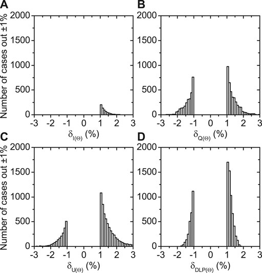
We computed 160 scattering angles $\text{Θ}$ between $-{65}^{\circ }$ and ${65}^{\circ }$ for the $\mathrm{3,024}$ cases, resulting in $\mathrm{483,840}$ test points, and we compared the simulated truth values of I, Q, U, and DLP for each of them to the corresponding values computed with each of the two LUTs. We found that for all $\mathrm{483,840}$ test values the SIR LUT reached the $\pm 1\text{\%}$ precision for all the Stokes parameters. The SK LUT demonstrated precision better than $\pm 1\text{\%}$ only at wavelength $\lambda =0.355\mu \text{m}$.

Figure 11 shows the results of comparisons for the SK LUT at $\lambda =2.264\mu \text{m}$, but again only for the tests that failed to reach the $1\text{\%}$ precision. The $\pm 1\text{\%}$ test failed 642 times for I ($0.13\text{\%}$; see panel (A) of Figure 11), $\mathrm{6,663}$ times for Q ($1.38\text{\%}$; see panel (B) of Figure 11), $\mathrm{7,817}$ times for U ($1.62\text{\%}$; see panel (C) of Figure 11), and $\mathrm{8,533}$ times for DLP ($1.76\text{\%}$; see panel (D) of Figure 11). Figure 11 confirms that degradation with increasing wavelength is a general feature of the SK LUT and the increase of wavelength has negative impact on the precision of estimations.

FIGURE 11

FIGURE 11. Selected Stokes parameters. Overview of the SK LUT outliers at $\lambda =2.264\mu \text{m}$. Description of labels is given in text.

With these results we conclude that the performance of the SIR LUT for polarimeter observables stays within $\pm 1\text{\%}$ without degrading at increasing wavelength. Also, as another conclusion, it is interesting to see that precise computation of Stokes parameters requires fewer radii grid bins compared to the elements of the normalized scattering matrix and lidar observables.

5 Conclusion

The SIR LUT provides an improved aerosol inherent optical properties LUT that can be used with advanced lidar and polarimeter aerosol microphysical retrievals as well as other remote sensing and in situ applications. Depending on the aerosol IOP, the SIR LUT improves precision by up to $34\text{\%}$ compared to the SK LUT. The design of the LUT takes into account mathematical features of Lorenz-Mie scattering theory and can be applied to a range of wavelengths starting at $0.355\mu \text{m}$ and a range of aerosol PSDs. The theoretical background of the LUT design was published as a minor part of earlier studies. In this contribution we attempted to provide a complete and thorough description of the most important mathematical aspects of the SIR LUT.

We introduced several theoretical and practical improvements to the existing LUT approach. We implemented quadratic approximation of the aerosol PSD since we found it improves precision over linear approximation. The new irregular angular quadrature allows us to use fewer scattering angles and improves precision at the same time. The range of size parameters was widened and now covers values from $\sim 0.018$ to $\sim \mathrm{1,770}$. Due to our access to superior computational hardware, we also increased the number of radius quadrature points to the extent that it fulfills the conditions of Nyquist–Shannon–Kotelnikov sampling theorem. The larger number of radius quadrature points solves the SK LUT’s issue that causes degraded accuracy and precision of the aerosol IOPs as the wavelength increases.

For verification, we used two reliable Lorenz-Mie single-scattering programs developed by two independent and well established scientific groups in the field of light scattering by small particles. One program was used to compute the coefficients of the SIR LUT itself at the reference wavelength of $0.355\mu \text{m}$. The other program was used to compute the simulated truth data at twelve wavelengths of interest via direct integration of the aerosol PSD using Simpson’s rule. Aerosol IOPs computed from the SIR LUT are precise to within $\pm 1\text{\%}$ with the exception that $P_{12}\left(\text{Θ}\right)$ is precise to within $\pm 2.5\text{\%}$ when the imaginary part of the CRI is below ${10}^{-5}$. As anticipated, the shortest tested wavelength delivers the least precise results in terms of aerosol IOPs and the precision of the SIR LUT improves as the wavelength increases. Further improvements in the precision of IOPs will likely require more radius quadrature points and denser coverage of the CRI that will increase the size of the SIR LUT.

Overall, the precision of aerosol IOPs computed from the SIR LUT is nearly equivalent to direct integration of the PSD using Simpson’s rule with $2\times {10}^7$ of logarithmically equidistant radius quadrature points from ${10}^{-3}$ to $100\mu \text{m}$, but can be used to make calculations about $\mathrm{1,000}$ times as quickly. The SIR LUT and examples of its use in several programming languages including C++, Fortran, Matlab, and Python are publicly available for the benefit of community at the web page https://science.larc.nasa.gov/polarimetry.

Data Availability Statement

The datasets presented in this study can be found in online repositories. The names of the repository/repositories and accession number(s) can be found below: https://science.larc.nasa.gov/polarimetry.

Author Contributions

Look-up table design and theory development: EC, SS, OD. Look-up table balancing between the size and precision: EC, SS, XL, BC. Quality control: SS, SB, CH, RF. Text: all authors. Grammar and wording improvements: SB, SS.

Funding

This research was partially funded by a NASA Remote Sensing Theory award.

Conflict of Interest

Author EC is employed by Science Systems and Applications, Inc.The remaining authors declare that the research was conducted in the absence of any commercial or financial relationships that could be construed as a potential conflict of interest.

Publisher’s Note

All claims expressed in this article are solely those of the authors and do not necessarily represent those of their affiliated organizations, or those of the publisher, the editors and the reviewers. Any product that may be evaluated in this article, or claim that may be made by its manufacturer, is not guaranteed or endorsed by the publisher.

Acknowledgments

The authors acknowledge the support of NASA LaRC K-Cluster staff, and thank Steven H. Carrithers in particular for his expert support in scientific computing. The authors also thank reviewers for their useful feedback leading to improvements of this work.

References

Bohren, C. F., and Huffman, D. R. (1983). Absorption and Scattering of Light by Small Particles. New York: John Wiley & Sons.

Burton, S. P., Hostetler, C. A., Cook, A. L., Hair, J. W., Seaman, S. T., Scola, S., et al. (2018). Calibration of a High Spectral Resolution Lidar Using a Michelson Interferometer, with Data Examples from ORACLES. Appl. Opt. 57, 6061–6075. doi:10.1364/ao.57.006061

PubMed Abstract | CrossRef Full Text | Google Scholar

Cairns, B., Russell, E. E., and Travis, L. D. (1999). Research Scanning Polarimeter: Calibration and Ground-Based Measurements. Proc. SPIE 3754, 186–196.

Google Scholar

Dubovik, O., Holben, B. N., Lapyonok, T., Sinyuk, A., Mishchenko, M. I., Yang, P., et al. (2002a). Non-spherical Aerosol Retrieval Method Employing Light Scattering by Spheroids. Geophys. Res. Lett. 29 (10). doi:10.1029/2001gl014506

CrossRef Full Text | Google Scholar

Dubovik, O., Lapyonok, T., Litvinov, P., Herman, M., Fuertes, D., Ducos, F., et al. (2014). GRASP: A Versatile Algorithm for Characterizing the Atmosphere. Newsroom: SPIE.

Dubovik, O., Herman, M., Holdak, A., Lapyonok, T., Tanré, D., Deuzé, J. L., et al. (2011). Statistically Optimized Inversion Algorithm for Enhanced Retrieval of Aerosol Properties from Spectral Multi-Angle Polarimetric Satellite Observations. Atmos. Meas. Tech. 4, 975–1018. doi:10.5194/amt-4-975-2011

CrossRef Full Text | Google Scholar

Dubovik, O., Holben, B., Eck, T. F., Smirnov, A., Kaufman, Y. J., King, M. D., et al. (2002b). Variability of Absorption and Optical Properties of Key Aerosol Types Observed in Worldwide Locations. J. Atmos. Sci. 59, 590–608. doi:10.1175/1520-0469(2002)059<0590:voaaop>2.0.co;2

CrossRef Full Text | Google Scholar

Dubovik, O., and King, M. D. (2000). A Flexible Inversion Algorithm for Retrieval of Aerosol Optical Properties from Sun and Sky Radiance Measurements. J. Geophys. Res. 105, 20673–20696. doi:10.1029/2000jd900282

CrossRef Full Text | Google Scholar

Dubovik, O., Sinyuk, A., Lapyonok, T., Holben, B. N., Mishchenko, M., Yang, P., et al. (2006). Application of Spheroid Models to Account for Aerosol Particle Nonsphericity in Remote Sensing of Desert Dust. J. Geophys. Res. 111, D11208. doi:10.1029/2005jd006619

CrossRef Full Text | Google Scholar

Hansen, J. E., and Travis, L. D. (1974). Light Scattering in Planetary Atmospheres. Space Sci. Rev. 16, 527–610. doi:10.1007/bf00168069

CrossRef Full Text | Google Scholar

Kolmogorov, A. N. (1941). About the Logarithmic-normal Law of Particle Size Distribution during Crushing. Proc. USSR Acad. Sci. 31 (2), 99–101.

Google Scholar

Lüke, H. D. (1999). The Origins of the Sampling Theorem. IEEE Commun. Mag. 37 (4), 106–108. doi:10.1109/35.755459

CrossRef Full Text | Google Scholar

Mishchenko, M. I. (2019). Double-precision Lorenz-Mie Program for the Case of a Nonabsorbing Host Medium. Available at http://www.giss.nasa.gov/staff/mmishchenko/Lorenz-Mie.html.

Mishchenko, M. I., Travis, L. D., and Lacis, A. A. (2002). Scattering, Absorption and Emission of Light by Small Particles. Cambridge: Cambridge University Press.

Mishchenko, M. I. (2006). Scale Invariance Rule in Electromagnetic Scattering. J. Quantitative Spectrosc. Radiative Transfer 101, 411–415. doi:10.1016/j.jqsrt.2006.02.047

CrossRef Full Text | Google Scholar

National Academies of Sciences, Engineering, and Medicine (2018). Thriving on Our Changing Planet: A Decadal Strategy for Earth Observation from Space. Washington, DC: The National Academies Press.

Seinfeld, J. H., and Pandis, S. N. (2006). Atmospheric Chemistry and Physics. From Air Pollution to Climate Change. Hoboken: John Wiley & Sons.

Stamnes, S., Hostetler, C., Ferrare, R., Burton, S., Liu, X., Hair, J., et al. (2018). Simultaneous Polarimeter Retrievals of Microphysical Aerosol and Ocean Color Parameters from the "MAPP" Algorithm with Comparison to High-Spectral-Resolution Lidar Aerosol and Ocean Products. Appl. Opt. 57, 2394–2413. doi:10.1364/ao.57.002394

PubMed Abstract | CrossRef Full Text | Google Scholar

Thomalla, E., and Quenzel, H. (1982). Information Content of Aerosol Optical Properties with Respect to Their Size Distribution. Appl. Opt. 21, 3170–3177. doi:10.1364/ao.21.003170

PubMed Abstract | CrossRef Full Text | Google Scholar

Twomey, S. A. (1977). Introduction to the Mathematics of Inversion in Remote Sensing and Indirect Measurements. Amsterdam: Elsevier.

Van de Hulst, H. C. (1981). Light Scattering by Small Particles. New York: Dover.