The Directly-Georeferenced Hyperspectral Point Cloud: Preserving the Integrity of Hyperspectral Imaging Data

The raster data model has been the standard format for hyperspectral imaging (HSI) over the last four decades. Unfortunately, it misrepresents HSI data because pixels are not natively square nor uniformly distributed across imaged scenes. To generate end products as rasters with square pixels while preserving spectral data integrity, the nearest neighbor resampling methodology is typically applied. This process compromises spatial data integrity as the pixels from the original HSI data are shifted, duplicated and eliminated so that HSI data can conform to the raster data model structure. Our study presents a novel hyperspectral point cloud data representation that preserves the spatial-spectral integrity of HSI data more effectively than conventional square pixel rasters. This Directly-Georeferenced Hyperspectral Point Cloud (DHPC) is generated through a data fusion workflow that can be readily implemented into existing processing workflows used by HSI data providers. The effectiveness of the DHPC over conventional square pixel rasters is shown with four HSI datasets. These datasets were collected at three different sites with two different sensors that captured the spectral information from each site at various spatial resolutions (ranging from ∼1.5 cm to 2.6 m). The DHPC was assessed based on three data quality metrics (i.e., pixel loss, pixel duplication and pixel shifting), data storage requirements and various HSI applications. All of the studied raster data products were characterized by either substantial pixel loss (∼50–75%) or pixel duplication (∼35–75%), depending on the resolution of the resampling grid used in the nearest neighbor methodology. Pixel shifting in the raster end products ranged from 0.33 to 1.95 pixels. The DHPC was characterized by zero pixel loss, pixel duplication and pixel shifting. Despite containing additional surface elevation data, the DHPC was up to 13 times smaller in file size than the corresponding rasters. Furthermore, the DHPC consistently outperformed the rasters in all of the tested applications which included classification, spectra geo-location and target detection. Based on the findings from this work, the developed DHPC data representation has the potential to push the limits of HSI data distribution, analysis and application.

Introduction

In the era of machine learning, the wealth of spatial-spectral information provided by hyperspectral imaging (HSI) data presents a unique opportunity to model and understand complex dynamics in a variety of applications (Eismann, 2012). For instance, airborne long-wave infrared HSI data have been successfully used for mineral exploration, mining and geohazard monitoring through the detection of rock forming and alteration minerals (Riley and Hecker, 2013). In vegetation studies for example, visible and near-infrared airborne HSI data have been used with thermal imagery for the early detection of Xylella fastidiosa, a pathogenic floral bacterium (Poblete et al., 2020). The success of these applications, in addition to many others, rely on the use of various cutting-edge analytical techniques that have been specifically developed to exploit HSI data and its unique properties. For instance, the high dimensionality of HSI data can be leveraged using deep feature extraction techniques (Chen et al., 2016; Rasti et al., 2020) that transform raw data in a hierarchical fashion to a lower dimensional data representation composed of new variables that are more discriminant, abstract and robust. Challenges from spectral mixing in HSI data can be minimized using dictionary learning-based unmixing approaches (Hong et al., 2019; Liu et al., 2019) to understand the material composition of a single pixel. Even in the presence of signal noise, targets of interest can readily be detected using ensemble learning techniques (Zhao et al., 2019; Sun et al., 2020) and classified using graph convolutional neural networks (Qin et al., 2019; Hong et al., 2020a).

In order to obtain spatially coherent HSI data that optimally preserves the captured spectral information from the conventional sensor types (e.g., pushbroom and whiskbroom) used on unmanned aerial systems (UAS) (e.g., Lucieer et al., 2014; Arroyo-Mora et al., 2019; Arroyo-Mora et al., 2021) and manned airborne platforms (e.g., Kalacska et al., 2016), the geometric correction is essential. In the geometric correction, each pixel of acquired HSI data is located in a real-world coordinate space at the intersection of an input digital surface model (DSM) and a straight line that is projected from the sensor position at the pixel dependent look direction (Müller et al., 2002; Schroth, 2004; Yeh and Tsai, 2011; Lenz et al., 2014). The look direction describes the angle from which incoming electromagnetic radiation is observed by a particular pixel of the imager (Müller et al., 2002). It is calculated by accounting for the roll, pitch and yaw while simultaneously considering the focal geometry and boresight misalignment of the imaging system (Müller et al., 2002; Warren et al., 2014). The DSMs used to geometrically correct HSI data are typically derived from either Light Detection and Ranging (LiDAR) (Liu, 2008), radar altimetry (Leslie, 2018) or Structure-from-Motion photogrammetry (Westoby et al., 2012).

Due to various factors (e.g., lens distortion, sensor movement, rugged terrains) pixels in the imagery are not uniformly spaced over the imaged scene after the geometric correction (Galbraith et al., 2003; Vreys et al., 2016). To correct for this non-uniformity, the geometrically corrected data are often resampled on a north-oriented linear grid. Each cell in this grid is typically separated by an equal distance in both the easting and northing directions, leading to a raster with square pixels (Shlien, 1979; Richards and Jia, 1999; Warren et al., 2014).

When spatially resampling HSI data, the nearest neighbor resampling method is conventionally applied (Roy, 2000; Williams et al., 2017). In this technique, the spectrum for each cell in the pre-specified linear grid is determined by the nearest spectrum from the geometrically corrected imaging data that are being resampled (Shlien, 1979). Since this resampling process does not change the value recorded in any given spectrum, the nearest neighbor methodology preserves spectral data integrity (Schläpfer et al., 2007). Nonetheless, the nearest neighbor method can compromise spatial data integrity. For instance, nearest neighbor resampling can lead to a blocky appearance due to pixel duplication if oversampling occurs (Arif and Akbar, 2005). Likewise, if the data are undersampled during nearest neighbor resampling, pixels can be lost all together, eliminating valid spectral information (Arif and Akbar, 2005). Even if pixel duplication and loss are near zero, nearest neighbor resampling shifts the position of each pixel (Shlien, 1979; Roy, 2000), altering the calculated location of each spectral measurement.

In many of the popular sensor designs (e.g., pushbroom and whiskbroom) the spatial characteristics of collected HSI data are often different between the cross track and along track directions (Inamdar et al., 2020). Therefore, it is difficult to select a spatial resolution for the resampling grid used in the nearest neighbor methodology. Figure 1 illustrates this issue, showing the spatial resampling process for theoretical HSI data. In this example, the pixel spacing in the cross track is half that of the along track. If the imagery is resampled to the cross track pixel spacing, there would likely be a substantial amount of pixel duplication due to oversampling in the along track (Figure 1A). In the alternative case where the imagery is resampled to the along track pixel spacing, there would be a considerable amount of pixel loss due to undersampling in the cross track (Figure 1B). The impact of pixel loss and duplication on remote sensing applications has not been addressed in the literature. Regardless of the method, resampling will affect the spatial integrity of HSI datasets so that the end product fits a raster data structure (Shlien, 1979).

FIGURE 1

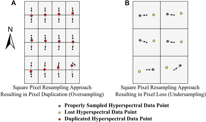
FIGURE 1. Pixel loss and pixel duplication during nearest neighbor spatial resampling. Consider spatially resampling a hyperspectral imaging dataset (given by the colored circles) acquired along an approximate true north heading where the pixel spacing in the cross track is half that of the along track. To generate a rasterized data product (given by the grey raster grid and the small black dots which designate the center of each cell), the data must be resampled on a north-oriented grid. Panels (A) and (B) show two resampling grids that could be used for the nearest neighbor resampling.

Instead of the conventional raster data structure, hyperspectral data can be represented as a point cloud, where each spectrum has a distinct position in a three-dimensional space. Hyperspectral point clouds have been extensively discussed in the remote sensing literature. Hyperspectral point cloud generation methodologies can be grouped into three main categories (Brell et al., 2019): 1) physical measurements that collect simultaneous hyperspectral and surface elevation data from a single sensor (e.g., Vauhkonen et al., 2013), 2) photogrammetric ranging with multiple full-frame hyperspectral images (e.g., Oliveira et al., 2019) and 3) data fusion that synergistically integrates surface elevation data with conventional HSI data (e.g., Brell et al., 2019). With physical measurements, it is critical to recognize that a single airborne sensor is not capable of collecting both high quality spectral and elevation data (Brell et al., 2019), especially at fine spectral-spatial resolutions. With photogrammetric ranging, the data storage requirements can pose operational and computational difficulties, especially at high spatial resolutions (< 3 cm) over large extents since a large volume of data are collected due to the necessity of multiple images with significant overlap. There can also be fundamental issues with photogrammetric ranging hyperspectral point cloud generation related to spectral data integrity depending on the manner in which the spectral information is assigned to each calculated elevation point (Aasen et al., 2015). Data fusion utilizing separate surface elevation and HSI datasets are generally the most feasible, however, their spectral and spatial alignment is challenging due to different sampling strategies, interaction with surface objects and fundamental differences in sensor characteristics (e.g., spectral-spatial point spread functions, illumination sources and viewing angles) (Brell et al., 2016; Brell et al., 2017; Brell et al., 2019).

Despite the abundance of hyperspectral point cloud generation methods, raster datasets have remained the standard for HSI data for over 40 years (Vane et al., 1984; Wilkinson, 1996; Goetz, 2009). This is likely due to the aforementioned difficulties with hyperspectral point cloud generation approaches: they can be difficult to implement, computationally expensive, result in large file sizes and compromise spatial-spectral data integrity. Interestingly, when generating conventional raster images, a hyperspectral point cloud is generated as each hyperspectral pixel is assigned an easting, northing and elevation value during the geometric correction (Müller et al., 2002; Lenz et al., 2014). This point cloud information is rarely analyzed by end users, who are provided with the elevation removed, resampled HSI products in raster format. A data fusion workflow that is implemented via the geometric correction would be straightforward to implement in existing processing protocols. The lack of spatial resampling in such a data product would also mean that the point cloud would preserve the spatial-spectral integrity of HSI data more effectively than rasters.

The objective of our study is to propose a hyperspectral point cloud data representation that preserves the spatial-spectral integrity of HSI data more effectively than conventional square pixel raster end products. This data representation, the Directly-Georeferenced Hyperspectral Point Cloud (DHPC), is generated through a novel data fusion workflow that can be implemented with the same tools used to generate conventional rasters. Our work herein first describes four HSI datasets that we use to generate both raster and DHPC end products. This description incudes an overview of the implemented raster data processing workflow and the developed DHPC data fusion workflow. After, we assess the DHPC and raster data products based on three spatial integrity data quality metrics (i.e., pixel loss, pixel duplication and pixel shifting) and data storage requirements, which is an important parameter for data distribution. Finally, we assess the practical implications of the data quality metrics by comparing the DHPC end products against the conventional raster end products in common HSI applications including classification, spectra geo-location and target detection. Overall, our study proposes an alternative data representation to the conventional raster data model that has the potential to push the limitations of data distribution, analysis and application in HSI.

Materials and Methods

Data Collection and Processing

Study Areas

The study analyzed HSI data collected at three field sites with different topographic features: the Mer Blue Peatland (MBP), the Cowichan Garry Oak Preserve (CGOP) and the Parc National du Mont- Mégantic (MMG). These sites are important climate change and conservation study areas. The MBP is a ∼8,500 year old ombrotrophic bog in Ottawa, Ontario, Canada (Lafleur et al., 2001). It is characterized by a hummock-hollow microtopography that corresponds with spatial patterns in vegetation and hydrology (Malhotra et al., 2016). A hollow is a wetter low-lying area that is dominated by Sphagnum spp mosses, while a hummock is a drier elevated mound rising from the surface with a dense cover of vascular plants in addition to mosses (Lafleur et al., 2005; Eppinga et al., 2008). The CGOP is located near Duncan, British Columbia, Canada. The site is an endangered Garry Oak Meadow with an open forest and an understory composed of native grasses and herbaceous vegetation. At this site, there is a difference in elevation (>10 m) between the top of the canopy and the understory. The MMG field site is located in southern Québec, Canada. The site is composed of mixed northern hardwood and boreal forest stands. The elevation gradient at this site is relatively large in comparison to the other two sites, changing by more than 600 m within the 10 km² area surrounding the peak of the mountain (Savage and Vellend, 2015).

Hyperspectral Imaging Data

HSI data were acquired with two hyperspectral imagers: the micro-Compact Airborne Spectrographic Imager (µCASI-1920, ITRES, Calgary, AB, Canada) and the Compact Airborne Spectrographic Imager (CASI-1500, ITRES, Calgary, AB, Canada). The imagers were mounted on different airframes and captured spectral information at different spatial scales (∼1.5–3 cm and ∼0.5–2.5 m, respectively) over the visible-near infrared portion of the electromagnetic spectrum. The µCASI-1920 was mounted on a DJI Matrice 600 Pro UAS. It is a variable framerate pushbroom imager that collects spectral data across a 34.21° field of view over 288 spectral bands (401–996 nm) on a silicon-based focal plane array (Arroyo-Mora et al., 2019). The CASI-1500 was mounted in a Twin Otter fixed-wing aircraft. It is a variable frame rate, grating-based, pushbroom imager with a 39.8° field of view that collects spectral information over 288 spectral bands (366–1,053 nm) with a silicon-based charged coupled device detector (Soffer et al., 2019). Both µCASI-1920 and CASI-1500 HSI data were collected over the MBP. µCASI-1920 data were collected at the CGOP site and CASI-1500 data were collected at the MMG site. Table 1 lists the parameters associated with both the µCASI-1920 and CASI-1500 datasets. The CGOP and MMG HSI data represented terrains with large elevation gradients relative to the sensor altitude and nominal pixel sizes of the imagery.

TABLE 1

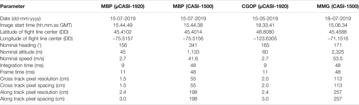
TABLE 1. Parameters for the hyperspectral imaging data acquired over the Mer Bleue Peatland (MBP), the Cowichan Garry Oak Preserve (CGOP) and the Parc National du Mont- Mégantic (MMG) with the µCASI-1920 and the CASI-1500. Nominal altitudes are reported as height above ground level.

The raw hyperspectral data were radiometrically and atmospherically corrected. The radiometric correction was implemented with proprietary software developed by the sensor manufacturer while the atmospheric correction was done using ATCOR4 [as described in Soffer et al. (2019)]. The MMG imagery further had a Lambert + Statistical-Empirical BRDF topographic correction applied (Richter and Schläpfer, 2020).

Conventional Hyperspectral Imaging Data (Square Pixel Raster)

To generate conventional HSI end products (georeferenced raster with square pixels), the radiometrically and atmospherically corrected data were first geometrically corrected and then spatially resampled. The geometric correction was completed with proprietary software from the sensor manufacturer using the onboard inertial navigation system data (position and attitude). The DSMs used for the geometric correction are described in Digital Surface Models. Conventional square pixel raster images were generated for each HSI dataset by spatially resampling the geometrically corrected HSI data on a north-oriented linear grid using a nearest neighbor methodology. Since there was a discrepancy between the cross track and along track pixel spacing of the collected HSI data, each HSI dataset was resampled on two different grids. Adjacent grid cells were separated by the cross track pixel spacing in the first resampling grid and the along track pixel spacing in the second resampling grid. Since the along track spacing was consistently larger than that of the cross track, the first resampling grid oversampled the data while the second undersampled the data to generate raster data products with square pixels. In total 8 imaging data sets were generated (two images for each of the HSI datasets described in Table 1).

Directly-Georeferenced Hyperspectral Point Cloud

The DHPC data fusion workflow implements a standard geometric correction processing protocol to create the point cloud (Figure 2). The workflow has three major inputs: the atmospherically corrected HSI data, the inertial navigation data of the sensor (position and attitude) and a DSM of the area covered by the HSI data.

FIGURE 2

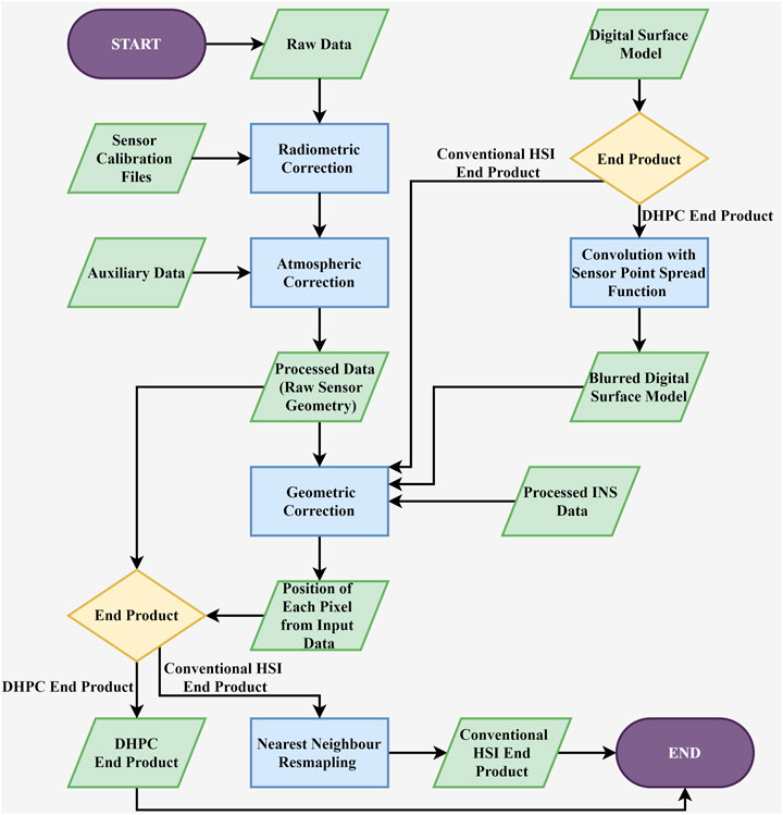
FIGURE 2. Flow chart of the hyperspectral imaging (HSI) processing workflow for both conventional rasterized hyperspectral imaging end products and the Directly-Georeferenced Hyperspectral Point Cloud (DHPC).

The first step in the DHPC data fusion workflow modifies the input DSM, blurring it through convolution with the point spread function of the imaging sensor. This modification makes the spatial properties of the DSM more consistent with the collected HSI data; each point in the blurred DSM corresponds to the average elevation of the objects/terrain that would contribute to a single HSI pixel.

In the second and final step of the data fusion workflow, the HSI data in its original sensor geometry is projected onto the blurred DSM. This was practically done by applying the geometric correction described in Conventional Hyperspectral Imaging Data (Square Pixel Raster), using the blurred DSM instead of the original. As a result of the blurred DSM, each HSI pixel receives the average surface elevation of the materials contributing to it. With the real-world position (northing, easting, averaged surface elevation) of each pixel from the imagery in its original sensor geometry, the DHPC is complete. In our study, each point in the DHPC data product was referred to as a “pixel”. Following the described workflow, a DHPC was generated for each of the HSI datasets from Table 1.

Digital Surface Models

The DSMs used to geometrically correct the µCASI-1920 data were generated by using a Structure-from-Motion Multiview Stereo (SfM-MVS) workflow from RGB photography (Kalacska et al., 2017; Kalacska et al., 2020). In this workflow (Lucanus and Kalacska, 2020) geo-tagged aerial photographs were collected on June 6th, 2019 (for MBP) and May 11th, 2019 (for CGOP) over the area covered by the µCASI-1920 imagery, with a Canon EOS 5D Mark III equipped with a Canon EF 24–70 mm f/2.8 L II USM lens set to a focal length of 24 mm. All photographs included the geolocation and altitude of the UAS, as recorded by an EMLID Reach M+ GNSS module. The collected raw GNSS data were postprocessed with RTKLIB (Takasu and Yasuda, 2009) using local base station data collected from a EMLID Reach RS+ GNSS module that was receiving incoming corrections from a commercial NTRIP (Networked Transport of Radio Technical Commission for Maritime Services via Internet Protocol) casting service (Smartnet North America, Atlanta) on an RTCM3-iMAX (Radio Technical Commission for Maritime Individualized Master Auxiliary) mount point that used both GPS and GLONASS constellations. The SfM-MVS workflow was implemented using Pix4D Mapper Pro [see Kalacska et al. (2020) for details], ultimately generating a DSM at a spatial resolution of 0.69 cm for the MBP and 1.52 cm for the CGOP.

For the MBP CASI-1500 data, airborne LiDAR data collected for the National Capital Commission in 2009 (density 2–4 pts m²) (Arroyo-Mora et al., 2018b) were used to generate a DSM at a spatial resolution of 0.5 m. Based on ground observations and peat growth modeling, the MBP has been estimated to grow < 0.5 m over the last millennium (Frolking et al., 2010). Given this slow growth rate, the LiDAR data collected in 2009 is still appropriate to apply to the peatland.

For the MMG CASI-1500 data, the study used airborne LiDAR data collected in 2018 by the Ministry of Forests, Wildlife and Parks of Québec as part of the province-wide LiDAR sensor data acquisition project (density 2.5 pts m²) (Le ministère des Forêts, de la Faune et des Parcs, 2021). The dataset was provided as a DSM at a spatial resolution of 1 m.

Data Assessment Metrics

Three spatial data quality metrics were calculated for each DHPC and square pixel raster end product: pixel loss (PL), pixel duplication (PD) and root mean square error in the radial direction (RMSE_r). PL (%) is the total percentage of pixels from the original HSI dataset that were not used in the final data product. PD (%) is the total percentage of pixels in the final data product that are duplicates. The RMSE_r gives a measure of the average distance (cm) the location of each pixel (as determined from the geometric correction) was shifted while generating the final end product. Assuming a uniform pixel spacing in the cross track and along track directions, it is possible to derive theoretical PL and PD values (see Theoretical Pixel Loss and Pixel Duplication Derivation) for any given HSI dataset from nominal flight parameters alone. Following this derivation, theoretical PL (PL_H) and PD (PD_H) values were calculated for each of the resampled and DHPC datasets and compared to the measured values. In addition to the described spatial data quality metrics, data storage requirements for each DHPC and square pixel raster end product were also calculated.

Pixel Loss

The PL was calculated according to Mulcahy (2000) (Eq. 1):

$PL=\left(1-\frac{U_{I_r}}{T_{I_o}}\right)\times 100\%(1)$

where the following holds: $U_{I_r}$ represents the number of unique spectra in the analyzed data product (I_r) and $T_{I_o}$ represents the number of total spectra in the original imagery from which I_r was derived. PL is given as a percentage, indicating the total percentage of pixels from the original HSI dataset that were not used in the final data product.

Pixel Duplication

The PD was calculated according to Mulcahy (2000) (Eq. 2):

$PD=\left(1-\frac{U_{I_r}}{T_{I_r}}\right)\times 100\%(2)$

where the following holds: $U_{I_r}$ represents the number of unique spectra in the analyzed data product (I_r) while $T_{I_r}$ represents the total number of spectra in I_r. PD is given as a percentage, indicating the total portion of pixels in I_r that are duplicates of one another.

Horizontal Linear Root Mean Square Error in Radial Direction

The RMSE_r was calculated according to American Society for Photogrammetric Engineering Remote Sensing (2015) (Eq. 3):

$RMS{E}_r=\sqrt{\frac{{{\displaystyle \sum }}_{i=1}^{i=n}({\left[P_{r,North}\left(S_r\left(i\right)\right)-P_{o,North}\left(S_r\left(i\right)\right)\right]}^2+{\left[P_{r,East}\left(S_r\left(i\right)\right)-P_{o,East}\left(S_r\left(i\right)\right)\right]}^2)}{n}}(3)$

where the following holds: S_r(i) represents the spectrum from the ith pixel of the analyzed data product (I_r); P_r,North(S_r(i)) represents the northing position of S_r(i) in I_r; P_r,East(I_r(i)), represents the easting position of S_r(i) in I_r; n represents the total number of spectrum in I_r; P_{o, North} (S_r(i)) represents the original northing position of S_r(i) as calculated during the geometric correction; and P_{o, East} (S_r(i)) represents the original easting position of S_r(i) as calculated during the geometric correction. The RMSE_r gives a measure of the average distance (cm) the location of each pixel (as determined by the geometric correction) is shifted in the final data product.

Theoretical Pixel Loss and Pixel Duplication Derivation

This section derives the theoretical PL (PL_H) and PD (PD_H) of a hypothetical HSI dataset ($I_o$) collected with uniform pixel spacing in the cross track and along track directions. In this section, $I_o$was assumed to be collected over an area with length W in the cross track direction and length L in the along track direction. Furthermore, the cross track pixel spacing (Ps_cross) was assumed to be smaller than that of the along track pixel spacing (Ps_along). The total number of spectra in $I_o$ ($T_{I_o}$) was approximated by the following:

$T_{I_o}=\left(L/P{s}_{along}\right)\left(W/P{s}_{cross}\right)(4)$

The theoretical PL and PD values were calculated for the two resampling approaches investigated in our study. The first resampling grid oversampled $I_o$ (resampling resolution equal to the cross track pixel spacing) while the second undersampled $I_o$ (resampling resolution equal to the along track pixel spacing). The total number of pixels in the resampled dataset can be calculated from:

$T_{I_r}=\left(L/R_r\right)\left(W/R_r\right),(5)$

where $R_r$ is the resolution of the resampled image ($I_r$).

Considering the first scenario (dataset is oversampled), it is assumed that there is no PL (PL_H = 0%) since $R_r$ is always equal to or smaller than pixel spacing throughout $I_o$. To derive PD_H, the number of total ($T_{I_r})$ and unique ($U_{I_r})$ spectra within the resampled image (I_r) must be calculated. Since there is no PL, $U_{I_r}$ is equal to $T_{I_o}$.

Starting from the PD formula given in Pixel Duplication, the derivation follows:

$P{D}_H=\left(1-\frac{U_{I_r}}{T_{I_r}}\right)\times 100\%(6)$

$P{D}_H=\left(1-\frac{\left(L/P{s}_{along}\right)\left(W/P{s}_{cross}\right)}{\left(L/P{s}_{cross}\right)\left(W/P{s}_{cross}\right)}\right)\times 100\%(7)$

$P{D}_H=\left(1-\frac{P{s}_{cross}}{P{s}_{along}}\right)\times 100\%(8)$

Considering the second scenario (dataset is undersampled), it is assumed that there is no PD (PD_H = 0%) since the resampling resolution is always equal to or greater than the pixel spacing throughout $I_o$. To derive PL_H, $T_{I_o}$ and $U_{I_r}$ are required. Since there is no PD, $U_{I_r}$ is equal to $T_{I_r}$

Starting from the PL formula given in Pixel Loss, the derivation follows:

$P{L}_H=\left(1-\frac{U_{I_r}}{T_{I_o}}\right)\times 100\%(9)$

$P{L}_H=\left(1-\frac{\left(L/P{s}_{along}\right)\left(W/P{s}_{along}\right)}{\left(L/P{s}_{along}\right)\left(W/P{s}_{cross}\right)}\right)\times 100\%(10)$

$P{L}_H=\left(1-\frac{P{s}_{cross}}{P{s}_{along}}\right)\times 100\%(11)$

The theoretical PL and PD of the DHPCs required no derivation; since pixels were not resampled after the geometric correction, there should be zero PL_H or PD_H.

Hyperspectral Imaging Data Applications

To compare the DHPC to the two resampled data products, two applications were tested with the MBP µCASI-1920 imagery. The first was a simple classification problem, differentiating two microforms (hummocks and hollows) in the MBP. The second µCASI-1920 application aimed to approximate the potential error in biomass estimation for hummocks and hollows (based on the classification results).

Two applications were also assessed for the MBP CASI-1500 data. The first located unique spectra within pre-specified vegetation plots. This application was based on common HSI end user requirements of matching ground control data (e.g., vegetation species counts) with HSI data (Arroyo-Mora et al., 2018a). The second CASI-1500 application was a sub-pixel target detection exercise.

Hummock and Hollow Classification (µCASI-1920)

Hummocks and hollows were classified from the MBP µCASI-1920 HSI data using a linear discriminant analysis (LDA) classification (Fisher, 1936). An independent classification model was trained and validated for each of the resampled µCASI-1920 images and the DHPC, resulting in nine different classification models. Each of the models were differentiated by the utilized training dataset (oversampled raster, undersampled raster or DHPC) and training variables (elevation only, spectral reflectance only or elevation and spectral reflectance). The surface elevation data for the rasterized data products were provided during geometric correction by resampling the surface elevation value associated with each pixel. The performance of each model was measured by the overall accuracy, producer’s accuracy and user’s accuracy metrics calculated on the validation dataset. The training and validation datasets for each model were generated based on both elevation and spectral data with domain knowledge of the MBP. In this process, trees were masked by removing the upper 2 percentile of the surface elevation distribution in each dataset. The surface elevation data were then detrended by removing the median surface elevation in a 10 × 10 m area around each pixel. Potential hummocks were identified as the 75–90^th percentile of the detrended surface elevation data. Potential hollows were identified as the bottom 5^th percentile. The identified hummocks and hollows were further filtered to remove bright (i.e., man-made objects) and low (i.e., shadows) reflectance objects. In this filtering, hummock and hollow labels that fell within the top and bottom 5 percentile of the spectral data at 600 nm were removed. Half of the remaining hollow labels were randomly selected and designated as training data. The other 50% of hollow labels were designated as validation data. An equal number of hummock data points were randomly selected and designated as training data and validation data. A minimum of 60,000 training and validation data points were used for each of the models.

Biomass Error Estimation for Hummocks and Hollows (µCASI-1920)

To assess the impact of resampling and the DHPC on a basic modeling question, our study investigated how classification errors could affect total aboveground biomass estimation. The biomass of hummocks and hollows were assumed to be Gaussian in nature. For hummocks, this Gaussian distribution was defined by a mean value of 527 g/m² and a standard deviation (SD) of 43 g/m². For hollows, this Gaussian distribution was defined by a mean value of 431 g/m² and a SD of 147 g/m². Each of these biomass distributions (mean and SD) were based on ground data from the MBP reported in Bubier et al. (2003).

A biomass value was randomly generated for each observation in the validation dataset based on its actual microform label. For instance, if an observation was actually labeled a hummock, it would be randomly assigned a biomass value from the previously defined hummock biomass distribution function. The mean of the randomly generated biomass values was calculated separately for hummocks and hollows based on the predicted labels in the validation dataset. In a perfect classification, the mean biomass of predicted hummocks and hollows would be nearly identical to the values used for the field-based biomass distributions. As such, to quantify the error in the biomass estimation for hummocks and hollows due to misclassification, the difference between the mean of the predicted and actual biomass distributions (ΔB_µ,mf) was calculated for both hummocks (ΔB_µ,hk) and hollows (ΔB_µ,hw).

Geo-Locating Spectra From Pre-Specified Vegetation Plots (CASI-1500)

One-hundred virtual 3 × 3 m vegetation plots were randomly placed across the MBP (uniform probability distribution over space). The mean number of spectra and unique spectra per plot were calculated in both the raster data sets and the DHPC generated from the CASI-1500. A pixel spectrum was located within a plot if its center was within the spatial boundaries of the plot. The percentage of these spectra located outside the plots before rasterization were calculated. The tested datasets were evaluated by identifying the mean number of unique spectra per plot that fell within its spatial boundaries before and after rasterization.

Detecting Sub-Pixel Targets (CASI-1500)

A target detection analysis was conducted on each of the MBP CASI-1500 datasets. One-thousand artificial targets were randomly placed across the MBP (uniform probability distribution over space). In sub-pixel detection applications, the position of a target within a pixel’s field of view and the sensor point spread function are of utmost importance (Radoux et al., 2016). As such, this application assumed that a target can be detected within a pixel of the imagery in its raw sensor geometry (pre-rasterization) if the point spread function of the pixel was greater than a pre-defined threshold value at the location of the target. The study tested threshold values ranging from 0.15 to 0.85 in increments of 0.05. The higher the threshold, the more difficult it was for a target to be detected within any given pixel of the imagery in its original sensor geometry. Based on this target detection, the false discovery rate and false negative rate were then calculated for each of the oversampled, undersampled and DHPC products. A pixel was a true positive if the detected target was within its spatial boundaries. For the rasterized data product, the spatial boundaries were given by their pixel boundaries. For the DHPC, the boundaries were given by the full width at half maximum (FWHM) of the sensor point spread function.

Results

Hyperspectral Imaging Data Assessment

Terrain With Small Elevation Gradient Relative to Sensor Altitude and Nominal Pixel Size

The MBP HSI data are displayed in Figures 3, 4. Table 2 records the RMSE_r, PL, PD, PL_H, PD_H and file size of the raster and point cloud datasets. The oversampled MBP data products were large in file size (30.90 Gb for µCASI-1920 and 40.36 Gb for CASI-1500) and characterized by high PD (50.25% for µCASI-1920 and 77.70% for CASI-1500). The PD for the oversampled CASI-1500 dataset was relatively large in comparison to the theoretical value (PD_H = 72.22%). The undersampled MBP data products were small (7.77 Gb for µCASI-1920 and 2.57 Gb for CASI-1500) and characterized by a large PL (51.09% for µCASI-1920 and 72.32% for CASI-1500). The RMSE_r for the resampled µCASI-1920 and CASI-1500 were 1.1 cm and 66.7 cm, respectively. The DHPC products for the MBP had a small file size (4.55 Gb for µCASI-1920 and 3.05 Gb for CASI-1500) and were characterized by zero PL, PD and RMSE_r. Supplementary Video S1, S2 show the DHPCs in three dimensions.

FIGURE 3

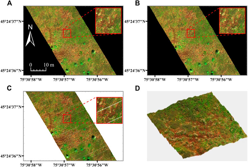
FIGURE 3. Hyperspectral imaging data (R = 639.6 nm, G = 550.3 nm, B = 459.0 nm) from the µCASI-1920 over the Mer Bleue Peatland. Panels (A, B) are rasterized hyperspectral imaging datasets resampled to 1.5 × 1.5 cm (A) and 3 × 3 cm (B). Panel (C) represents the Directly-Georeferenced Hyperspectral Point Cloud (DHPC) viewed from above. Panel (D) displays a video still of the DHPC in a 12 × 12 m region around the image zoom center. In all panels, each displayed band is linearly stretched between 0 and 12%. The full video can be seen in Supplementary Video S1. The white stripes in the DHPC [clearly visible in the image zoom of panel (C)] represent areas on the ground that were not sampled by the hyperspectral imager during data acquisition. These gaps are not present in the raster images (A, B) as they are interpolated over with duplicated pixels from the edges of the stripes during the nearest neighbor resampling.

FIGURE 4

FIGURE 4. Hyperspectral imaging data (R = 640.8 nm, G = 549.9 nm, B = 459.0 nm) for the CASI-1500 over the Mer Bleue Peatland. Panels (A, B) are rasterized hyperspectral imaging datasets resampled to 50 × 50 cm (A) and 200 × 200 cm (B) grids. Panel (C) represents the Directly-Georeferenced Hyperspectral Point Cloud (DHPC) viewed from above. Panel (D) displays a video still of the DHPC in a 240 × 240 m region surrounding the image zoom center. The full video can be seen in Supplementary Video S2. In all panels, each displayed band is linearly stretched between 0 and 12%.

TABLE 2

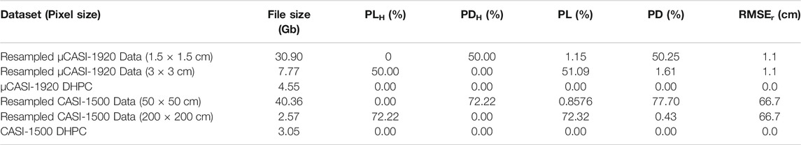
TABLE 2. The file size, pixel loss (PL), pixel duplication (PD), theoretical pixel loss (PL_H), theoretical pixel duplication (PD_H) and horizontal root mean square error (RMSE_r) in the radial direction for the µCASI-1920 and CASI-1500 data over the Mer Bleue Peatland. These data include the resampled hyperspectral imaging datasets and the Directly-Georeferenced Hyperspectral Point Clouds (DHPC).

Terrain With Large Elevation Gradient Relative to Sensor Altitude and Nominal Pixel Size

The CGOP and MMG HSI data are displayed in Figures 5, 6 and, respectively. Table 3 records the RMSE_r, PL, PD, PL_H, PD_H and file size of the raster and point cloud datasets. The oversampled CGOP and MMG data products were large in file size (24.40 Gb for CGOP and 30.67 Gb for MMG) and characterized by high PD (34.29% for CGOP and 59.76% for MMG). The oversampled CGOP dataset also had a relatively large PL of 11.09% in comparison to the theoretical value (PL_H = 0.00%). The undersampled CGOP and MMG data products were small in file size (10.89 Gb for CGOP and 5.54 Gb for MMG) and characterized by high PL (46.69% for CGOP and 58.12% for MMG). The PL for the undersampled CGOP dataset was relatively large in comparison to the theoretical value (PL_H = 33.33%). The undersampled MMG and CGOP data products also had relatively high PD (11.49% for CGOP and 5.52% for MMG) in comparison to the theoretical value (PD_H = 0.00%). The RMSE_r for the resampled CGOP and MMG data were 3.9 cm and 86.6 cm, respectively. The DHPC products for the CGOP and MMG sites had a small file size (10.16 Gb for CGOP and 4.73 Gb for MMG) and were characterized by zero PL, PD and RMSE_r. Supplementary Video S3, S4 show the DHPCs in three dimensions.

FIGURE 5

FIGURE 5. Hyperspectral imaging data (R = 639.6 nm, G = 550.3 nm, B = 459.0 nm) from the µCASI-1920 over the Cowichan Garry Oak Preserve. Panels (A, B) are rasterized hyperspectral imaging datasets resampled to 2 × 2 cm (A) and 3 × 3 cm (B) grids. Panel (C) represents the Directly-Georeferenced Hyperspectral Point Cloud (DHPC) viewed from above. Panel (D) displays a video still of the DHPC in a 24 × 24 m region surrounding the image zoom center. The full video can be seen in Supplementary Video S3. In all panels, each displayed band is linearly stretched between 0 and 22%. The white stripes in the DHPC [clearly visible in the image zoom of panel (C)] represent areas on the ground that were not sampled by the hyperspectral imager during data acquisition. These gaps are not present in the raster images (A, B) as they are interpolated over with duplicated pixels from the edges of the stripes during the nearest neighbor resampling.

FIGURE 6

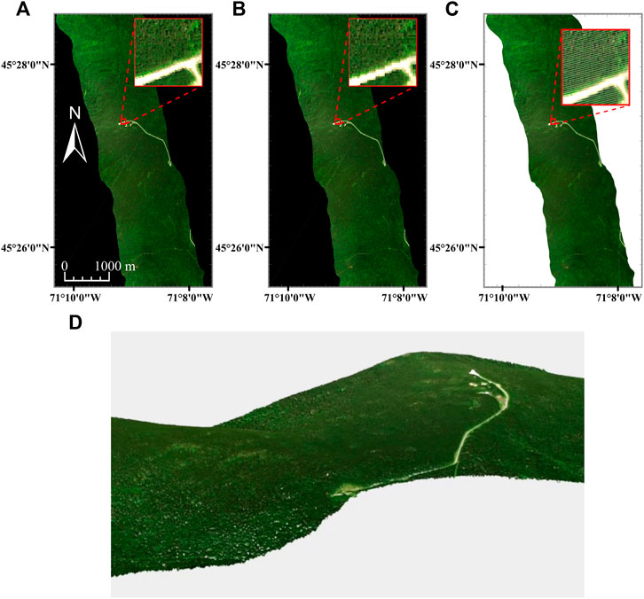
FIGURE 6. Hyperspectral imaging data (R = 640.8 nm, G = 549.9 nm, B = 459.0 nm) for the CASI-1500 over the Parc National du Mont- Mégantic. Panels (A, B) are rasterized hyperspectral imaging datasets resampled to 110 × 110 cm (A) and 260 × 260 cm (B) grids. Panel (C) represents the Directly-Georeferenced Hyperspectral Point Cloud (DHPC) viewed from above. Panel (D) displays a video still of the DHPC. The full video can be seen in Supplementary Video S4. In all panels, each displayed band is linearly stretched between 0 and 12%. The white stripes in the DHPC represent areas on the ground that were not sampled by the hyperspectral imager during data acquisition. The white stripes in the DHPC [clearly visible in the image zoom of panel (C)] represent areas on the ground that were not sampled by the hyperspectral imager during data acquisition. These gaps are not present in the raster images (A, B) as they are interpolated over with duplicated pixels from the edges of the stripes during the nearest neighbor resampling.

TABLE 3

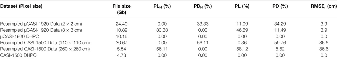
TABLE 3. The file size, pixel loss (PL), pixel duplication (PD), theoretical pixel loss (PL_H), theoretical pixel duplication (PD_H) and horizontal root mean square error (RMSE_r) in the radial direction for the µCASI-1920 data from the Cowichan Garry Oak Preserve and the CASI-1500 data from the Parc National du Mont- Mégantic. These data include the resampled hyperspectral imaging datasets and the Directly-Georeferenced Hyperspectral Point Clouds (DHPC).

Hyperspectral Imaging Data Applications

Hummock and Hollow Classification

The three models trained on the spectral data alone had the lowest overall classification accuracies (83.3–83.7%) (Table 4). Importantly, there was a discrepancy in these models between producer’s accuracy and user’s accuracy. For hollows, the user’s accuracies ranged from 86.3 to 86.8%. These values were higher than the producer’s accuracies which ranged from 79.1 to 79.6%. The opposite trend was observed for hummocks where the user’s accuracy ranged from 80.8 to 81.2% while the producer’s accuracy ranged from 87.4 to 87.9%. The models trained on the surface elevation data alone had overall accuracies of 85.8–86.5%. As with the spectral models, there was a discrepancy between user’s accuracy and producer’s accuracy. In hollows, the user’s and producer’s accuracies were valued at 82.4–83.0% and 91.1–91.8%, respectively. For hummocks, the user’s accuracy and producer’s accuracies were valued at 90.0–90.8% and 80.5–81.2%, respectively. The classification models trained on both the spectral and elevation data had the highest overall accuracy, user’s accuracy and producer’s accuracy values ranging from 90.0 to 91.3% for both hummocks and hollows. Although all classification accuracies were relatively constant when comparing models trained with identical variables, the DHPC based classification had higher overall accuracies by 0.3–0.7%.

TABLE 4

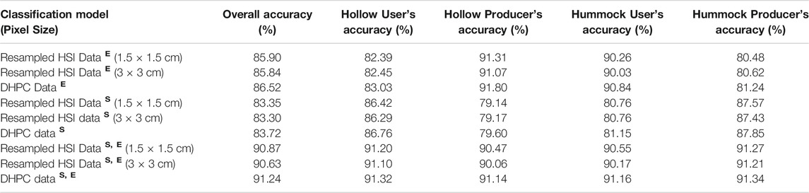
TABLE 4. Accuracy results for the hummock-hollow classification models (µCASI-1920 hyperspectral imaging (HSI) data from the Mer Bleue Peatland). Each of the models were differentiated by the training dataset and training variables. The training datasets included the Directly-Georeferenced Hyperspectral Point Cloud (DHPC) in addition to the three resampled hyperspectral images. The superscripts^{S, E} corresponded to the inclusion of the spectral reflectance and surface elevation, respectively.

The output classification map over a 12 × 12 m plot for each model is shown in Figure 7. When trained on spectral data alone (e.g., Figure 7H), the classification tracked hummocks and hollows observable in the RGB image (Figure 7J). Isolated hummock pixels were observed in hollow patches within the classification. The opposite was also observed, with isolated hollow pixels within hummock patches. These isolated pixels qualitatively decreased when using elevation data in addition to spectral data (e.g., Figure 7I), leading to a higher spatial coherency. There were few isolated pixels in the classification model trained on the surface elevation data alone. Nevertheless, there were clear areas of misclassification. For instance, in the north-west corner of the displayed classification map (e.g., Figure 7G), the entire region was classified as hummocks, despite the presence of hollows that can be seen in the RGB image (see Figure 7J) and surface elevation map (see Figure 7K).

FIGURE 7

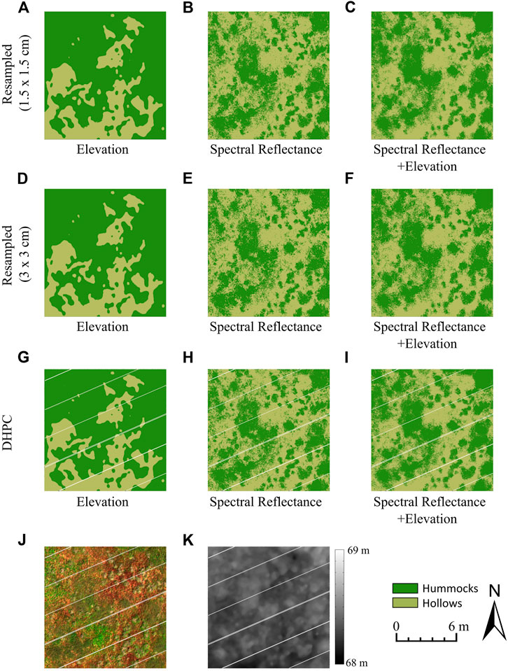
FIGURE 7. Panels (A-I) display sample hummock-hollow classification maps (12 × 12 m plot) generated from each of the trained models (µCASI-1920 HSI data from the Mer Bleue Peatland). The µCASI-1920 HSI data included the Directly-Georeferenced Hyperspectral Point Cloud (DHPC) in addition to the two resampled hyperspectral images. The hyperspectral dataset used to generate each panel is given by the row titles. The training variables used to generate each classification model were displayed in the subtitle below each panel. An RGB image (R = 639.6 nm, G = 550.3 nm, B = 459.0 nm, linearly stretched between 0 and 12%) and surface elevation map (linearly stretched from 68 to 69 m) were generated by viewing the DHPC from directly above and are displayed in panels (J) and (K), respectively. The hummocks appear green in panel (J) while hollows appear red. The white stripes in the DHPC data derivatives (G-K) represent areas on the ground that were not sampled by the hyperspectral imager during data acquisition. These gaps are not present in the raster data derivatives (A-F) as they are interpolated over with duplicated pixels from the edges of the stripes.

Biomass Error Estimation

The differences between the mean of the predicted and actual biomass distribution for both hummocks (ΔB_µ,hk) and hollows (ΔB_µ,hw) are displayed in Figure 8 (for exact values see Supplementary Table S1). The hollow distribution had a positive ΔB_µ,hw for all of the classification models. The opposite trend was observed in hummocks (ΔB_µ,hk<0). ΔB_µ,hw ranged from 12.72 to 13.18 g/m² for all models trained with the spectral data alone. ΔB_µ,hk ranged from −18.09 to −18.47 g/m² for all models trained with the spectral data alone. The models trained on the elevation data alone had the largest ΔB_µ,hw values (16.29–16.91 g/m²). In comparison to these values, the magnitude of the ΔB_µ,hk values when using elevation data alone were relatively small (8.79–9.56 g/m²). When using the classification models that incorporated both spectral and elevation information, both ΔB_µ,hw and ΔB_µ,hk decreased in magnitude; ΔB_µ,hw was equal to 8.34–8.54 g/m² while ΔB_µ,hk ranged from −8.48 to −9.45 g/m². Although all classification accuracies were relatively constant when comparing models trained with identical variables, the magnitude of ΔB_µ,hw and ΔB_µ,hk for the DHPC based classifications were always lower by 0.07–0.97 g/m².

FIGURE 8

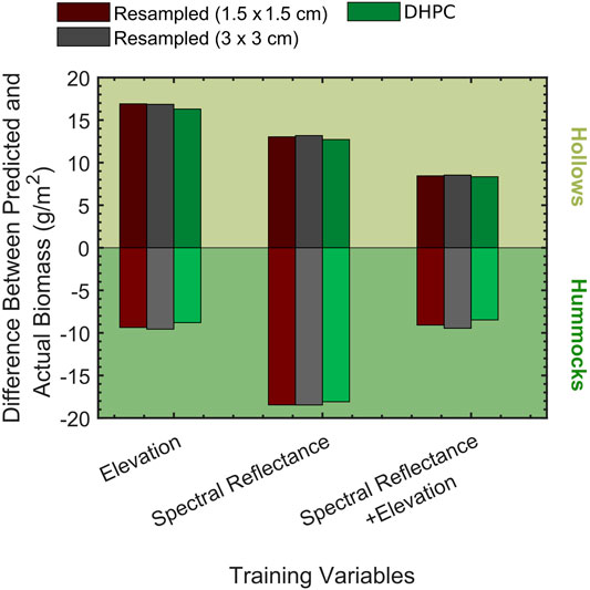
FIGURE 8. Biomass estimation errors (difference between mean of predicted and actual biomass) for the developed hummock hollow classification models for the µCASI-1920 hyperspectral imaging data from the Mer Bleue Peatland. This data included the Directly-Georeferenced Hyperspectral Point Cloud (DHPC) in addition to the two resampled hyperspectral images. Each of the models were differentiated by the training dataset (given by bar colours) and training variables. The bars above 0 correspond to hollow biomass estimation errors while the bars below correspond to hummocks.

Geo-Locating Spectra From Pre-Specified Vegetation Plots

The mean and SD of the number of CASI-1500 spectra located per vegetation plot is shown in Figure 9 (for exact values see Supplementary Table S2). For all resampled data products, spectra that were originally located outside the plot ended up within the boundaries of the plot after rasterization. The highest mean number of spectra located per plot (36.00) was acquired when oversampling the data. Approximately 62% of the identified spectra were duplicates of one another as there were only a mean of 13.56 unique spectra per plot. Approximately 38% of these unique spectra on average were from outside of the actual plots before rasterization. The lowest mean number of spectra located per plot (2.26) was acquired when undersampling the data. 100% of the located spectra were unique. On average, 40% of the spectra were originally from outside of the actual plots before rasterization. When using the DHPC, it was possible to locate a mean of 8.46 unique spectra per plot. With this technique, there was zero duplication in these spectra. Furthermore, none of the located spectra were originally from outside the actual plots.

FIGURE 9

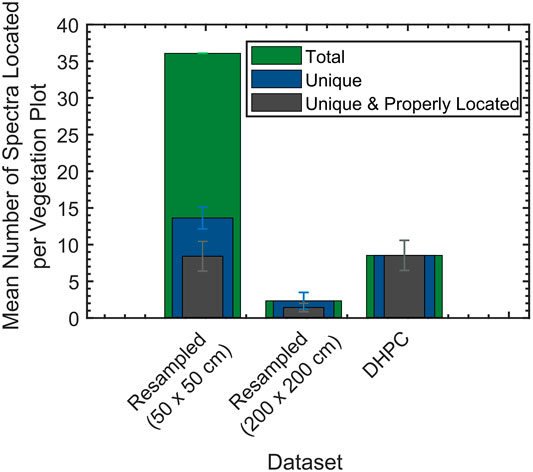
FIGURE 9. The mean and SD of the number of spectra, number of unique spectra and number of unique spectra properly located per each 3 × 3 m virtual vegetation plot (n = 100) from the Mer Bleue Peatland CASI-1500 data. The CASI-1500 data included the Directly-Georeferenced Hyperspectral Point Cloud (DHPC) in addition to the two resampled hyperspectral images. The error bars give the 1-sigma window around each mean value. Properly located spectra refer to those which were contained within each plot before and after rasterization (in the case of the resampled data products).

Detecting Sub-Pixel Targets

The results of the sub-pixel target detection (n = 1,000 targets) are displayed in Figure 10. The total number of identified targets decreased as the threshold value increased. The total number of targets identified were identical for the oversampled data product and the DHPC, decreasing from 1,000 at a threshold of 0.15 to 402 at a threshold value of 0.85. The undersampled data products detected 577 targets at a threshold of 0.15 and 88 at a threshold of 0.85. The false discovery rate decreased linearly as the applied threshold value increased for all data products. The false discovery rate of the oversampled data products decreased from 90% at a threshold value of 0.15 to 80% at a threshold value of 0.85. These false discovery rates were consistently larger than that of the undersampled data and the DHPC by an average of 50% and 69%, respectively. For all data products, the false negative rate increased linearly as the applied threshold value increased. The false negative rate was consistently largest for the undersampled data product increasing from 67% to 93% as the threshold value changed from 0.15 to 0.85. These false negative rates were consistently larger than that of the oversampled data and the DHPC by an average of 53% and 64%, respectively.

FIGURE 10

FIGURE 10. Target detection results from the CASI-1500 hyperspectral imaging data over the Mer Bleue Peatland. Artificial targets (n = 1,000) were randomly placed within the scene. The CASI-1500 data included the Directly-Georeferenced Hyperspectral Point Cloud (DHPC) in addition to the two resampled hyperspectral images. Panel (A) displays the number of targets (out of a maximum 1,000) identified in the target detection. Panel (B) and (C) give the false discovery and false negative rates, respectively.

Discussion

Our study presents a novel hyperspectral point cloud data representation which preserves the spatial integrity of HSI data (i.e., zero PL, PD and pixel shifting). Because the data fusion workflow does not modify the spectra from the original HSI data, the DHPC also preserves spectral data integrity. Although the raster datasets preserved spectral data integrity with the nearest neighbor methodology, spatial data integrity was compromised due to PL, PD and pixel shifting from the resampling. For the raster data products, there was a trade-off between PD and PL that was dependant on the resolution of the implemented resampling grid; oversampling resulted in substantial PD (∼35–75%) while undersampling led to substantial PL (∼50–75%) (Tables 2, 3). The PL and PD were primarily caused by the uneven pixel spacing between the cross track and along track directions. While it may be possible to collect data with nearly identical pixel spacing in the cross track and along track, there are practical limitations that make it difficult. For example, the pixel spacing in the along track is dependent on the integration time, frame time and platform speed, all of which have impacts on other aspects of the data such as the signal to noise ratio and positional accuracy (Arroyo-Mora et al., 2019; Inamdar et al., 2020). The PL and PD caused by nearest neighbor resampling have been analyzed in a limited number of remote sensing studies (e.g., Kimerling, 2002; Kollasch, 2005; Williams et al., 2017), with only one focusing on HSI data (Williams et al., 2017). However, it was outside the scope of these studies to quantify the negative effects of PD and PL.

In the resampled MBP and MMG data, the calculated PL and PD metrics were only marginally larger than the theoretical expectations (PD_H and PL_H) (Tables 2, 3). The PD and PD in the CGOP rasters exceeded theoretical expectations by up to ∼13%. The elevated PD and PL were likely a result of non-uniform pixel spacing due to differences in surface elevation across the scene. In the CGOP there was a difference in pixel spacing between the top of the canopy (∼1.5 cm in cross track) and the understory (∼2.0 cm in cross track). As such, even when resampling to 2.0 cm, the data were being undersampled at the top of the canopy, leading to PL. Due to the elevation of the surface relative to the sensor altitude, tall objects (e.g., treetop) blocked the view of lower lying regions of the imagery (e.g., ground below the canopy), leading to areas on the ground that were not imaged (data holes seen in Figure 5C). Such gaps are not present in the resampled images (Figures 5A,B) as they have been interpolated over with duplicated pixels from the edges, increasing PD values. The conservative assumptions made in Theoretical Pixel Loss and Pixel Duplication Derivation while deriving PD_H and PL_H likely mean that these metrics can be used to approximate the lower boundary of PL and PD. As such, PD_H and PL_H are valuable for flight planning efforts, allowing data collectors to avoid PL and PD in their datasets.

Regardless of whether the HSI dataset was undersampled or oversampled, pixel shifting was large in the studied rasters (RMSE_r = ∼0.33–1.33 pixels in the raster MBP and MMG data) in comparison to the DHPC. The RMSE_r values were, however, less than half the pixel spacing in the along and cross track directions and thus consistent with studies performed at the satellite level that quantify pixel shifting due to nearest neighbor resampling (e.g., Tan et al., 2006; Roy et al., 2016). Pixel shifting due to nearest neighbor resampling has been noted to negatively affect various applications [e.g., aligning multi-temporal datasets (Tan et al., 2006), change detection (Roy, 2000), classification (Alcantara et al., 2012) and biophysical parameter estimation (Tian et al., 2002)]. The exceptionally large RMSE_r values (∼1.30–1.95 pixels) in the CGOP was likely caused by the non-uniform pixel spacing across the scene due to large changes in elevation between treetops and ground below canopy relative to the sensor altitude.

In the DHPC data products (Figures 3–6), the observable white stripes represented areas on the ground that were not sampled by the hyperspectral imager during data acquisition. Such gaps in the imagery were likely caused by non-uniform sensor movement (e.g., sudden platform movement from changes in wind direction) between consecutive integration periods. It is important to recognize that these gaps are a true characteristic of the HSI data itself and are not data artifacts. Such gaps are not present in the resampled images as they have been interpolated over with duplicated pixels from the edges of the stripes. This example shows how the raster data model misrepresents HSI data as neighboring pushbroom HSI pixels in the along track direction are not uniformly spaced across the entire image.

In an ideal HSI end product, each pixel from the HSI data in its original sensor geometry should be sampled once. Since each pixel has identical data storage requirements (Johnson and Jajodia, 1998), an ideal HSI end product would have a file size roughly equal to that of the HSI data before the geometric correction (e.g., 4.09 Gb for the MBP µCASI-1920 data). In the rasterized data products, NoData pixels are abundant along the edges of the imagery (black pixels along the edges of Figures 6A,B). These additional NoData pixels contribute to the overall files size of raster data products (Lutes, 2005), increasing the data storage requirements. PD in the oversampled datasets led to a larger number of pixels, resulting in larger file sizes than in the ideal scenario (e.g., 30.90 Gb for the MBP µCASI-1920 data). Although the PL in the undersampled data product meant that many pixels were lost from the original HSI data in its raw sensor geometry (theoretically leading to smaller files sizes than in the ideal scenario), there were generally more pixels overall due to the presence of the NoData pixels. As such, even the undersampled datasets often had larger file sizes (e.g., 7.77 Gb for the MBP µCASI-1920 data) than in the ideal scenario. Even with its additional elevation data, the data storage requirements of the DHPC were only slightly larger than in the ideal scenario (e.g., 4.55 Gb for the MBP µCASI-1920 DHPC). The small file size was due to the absence of PD and NoData pixels along the edges of the imagery, making the DHPC ideal for data distribution. This is important given the data requirements of HSI, especially for high spatial resolution applications (Arroyo-Mora et al., 2019).

The DHPC outperformed the raster data products in the four studied applications. In the hummock-hollow classification, models trained with spectral data alone had the lowest overall accuracy (∼83%) and a discrepancy between user’s accuracy and producer’s accuracy. The discrepancy meant that there was a large portion of hollow pixels that were misclassified as hummocks, explaining why the magnitude of ΔB_µ,hk (∼18 g/m²) was larger than ΔB_µ,hw (∼13 g/m²) in the biomass error calculation. Models trained with the surface elevation data alone had an intermediate overall accuracy (∼86%). The discrepancy between user’s accuracy and producer’s accuracy in these models meant that the magnitude of ΔB_µ,hk (∼9 g/m²) was smaller than that of ΔB_µ,hw (∼17 g/m²) since a large portion of hummock pixels were being misclassified as hollows. The classification models trained on both the spectral and elevation data had high overall accuracy, user’s accuracy and producer’s accuracy for both hummocks and hollows (∼91%), leading to relatively low errors in biomass estimation (magnitude of ∼9 g/m²). These findings show that the integration of surface elevation and spectral information can lead to improved results for classification problems, agreeing with a number of other studies (e.g., Elaksher, 2008; Vauhkonen et al., 2013; Brell et al., 2019; Sothe et al., 2019; Hong et al., 2020b). For instance, Sothe et al. (2019) improved the overall accuracy of tree species classification of tropical forests by > 10% by using elevation data in addition to spectral information.

The DHPC based classification consistently had higher overall accuracies by 0.3–0.7% which led to lower biomass estimation errors by 0.07–0.97 g/m². The higher accuracies were likely due to the reduced levels of PL and PD, the latter of which has been found to impede classification accuracy (Chowdhury and Alspector, 2003). Based on the microform spatial distribution in the 19 km² region of MBP (Arroyo-Mora et al., 2018a), by implementing the DHPC, the aboveground biomass estimation of hollows (∼12.7% area coverage) and hummocks (∼51.2% area coverage) would be improved by 179–1,504 kg and 3,415–9,437 kg, respectively. Such a systematic increase in biomass estimation performance is biologically important since above ground biomass is one of the primary sources of carbon to peat soil and thus impacts the ability of peatlands to mitigate the effects of climate change by sequestering carbon (Moore et al., 2002).

In the geo-location application, a substantial portion of the located spectra in the raster data products originated from outside the plot before resampling (∼40%). These spectra were only brought within the plot due to the pixel shifting from resampling. If these spectra were used as training data in any remote sensing application, this could mean that a substantial amount of the training data would not be valid, potentially leading to error unrelated to the applied algorithm (Tan et al., 2006). When using the DHPC, 0% of the identified spectra were originally from outside the plots. By maximizing the total number of unique spectra located per plot, the DHPC should lead to improved performance in applications that rely on accurately matching field data to collected imagery [e.g., biophysical parameter estimation (Zhu et al., 2013) and classification (Alcantara et al., 2012)].

In the sub-pixel target detection application, a trade-off was observed between false discovery and false negative rates (Figure 10B,C). Such a trade-off is commonly discussed in the target detection literature (e.g., Han et al., 2014); false negatives increase while false discoveries decrease as target detection thresholds become more strict. The false discovery and false negative rates were linked to the PD and PL metrics (Figure 11). False discoveries were created when each true positive pixel was duplicated during resampling. Likewise, PL led to false negatives as true positive pixels were lost during resampling. These principles explain why the oversampled data product had a large false discovery rate and a low false negative rate while the opposite was observed in the undersampled data product. The DHPC minimized both false discovery rates (19% and 69% smaller on average than the undersampled and oversampled rasters, respectively) and false negative rates (11% and 64% smaller on average than the oversampled and undersampled rasters, respectively). The reduced error rates could allow individuals following up on target detection maps to identify more targets with less searching power, reducing cost and minimizing physical and environmental risks, [e.g., landmine detection (Makki et al., 2017) and invasive species detection (Pengra et al., 2007)]. In target detection applications where the precise location of a target is necessary, it may be problematic to use HSI data that is spatially resampled with the nearest neighbor approach. Further research should investigate the performance of target detection algorithms before and after spatial resampling.

FIGURE 11

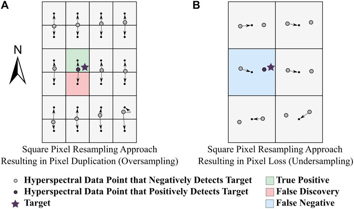
FIGURE 11. False discoveries and false negatives caused by pixel loss and pixel duplication in a target detection exercise. Consider spatially resampling a hyperspectral imaging dataset (given by the colored circles) acquired along an approximate true north heading where the pixel spacing in the cross track is half that of the along track. To generate a rasterized data product (given by the raster grid and the small black dots which designate the center of each cell), the data must be resampled on a north-oriented grid. In this scene there is one target of interest (purple star) that can be detected by the hyperspectral data point represented by the purple circle. Panel (A) shows that pixel duplication can cause false discoveries while panel (B) shows that pixel loss can cause false negatives.

In signature matched target detection algorithms, error metrics are often theoretically calculated based on the modeled probability distributions of the background and target signals. For reliable error metrics, the modeled distributions must accurately describe the data (Manolakis et al., 2016). There must also be a statistically significant number of target and background pixels. The availability of such datasets are often limited in the literature (Manolakis et al., 2013). In the theoretical target detection, the PSF was used as a detection statistic, fundamentally representing the horizontal distance from each pixel center to the nearest target. Since the location of each simulated target was known, it was possible to calculate error metrics from the target detection results, as opposed to modeled probability distributions. Such a target detection workflow is valuable in understanding the limitations of sub-pixel target detection and the variables that control it (e.g., size and position of a target within a pixel).

Aside from preserving spatial-spectral data integrity and the minimal data storage requirements, the DHPC is advantageous over other existing hyperspectral point clouds as its data fusion workflow can be implemented with the same tools used to process conventional raster end products. Additionally, the DHPC can use HSI and DSM data from a variety of different data sources and thus is not limited by any particular sensor. Furthermore, by convolving the DSM by the hyperspectral sensor PSF during the data fusion workflow, the spatial characteristics of the elevation data become more consistent with that of the HSI data. As such, the elevation information encoded in each pixel of the DHPC actually corresponds to the footprint of the spectral information, leading to a more spatially coherent data fusion. This convolution may come at the cost of fine spatial scale elevation information. Although there are hyperspectral point clouds that can preserve fine spatial scale elevation information, they can come at the cost of spectral data integrity, especially over spectrally and spatially heterogeneous terrains (Brell et al., 2019). Further research into the performance of the DHPC against other point cloud data representations is advised.

In this work, we developed a hyperspectral point cloud that preserves the spatial-spectral integrity of HSI data more effectively than conventional rasterized square pixel end products. Our DHPC methodology has been shown to produce no pixel shift, duplication or loss. Despite containing additional surface elevation data, the DHPC file size was up to 13 times smaller than the corresponding rasterized datasets. This is favorable for data distribution, especially since the DHPC generation workflow can be easily implemented with pre-existing processing protocols. Importantly, the DHPC consistently outperformed raster data products in various remote sensing applications (classification, target detection, spectra geolocation). Overall, our research shows that the developed DHPC data representation has the potential to push the limits of HSI data distribution, analysis and application.

Data Availability Statement

The datasets presented in this article are available from the corresponding author upon request following the CABO data use agreement from https://cabo.geog.mcgill.ca. Requests to access the datasets should be directed to Y2Fib3NjaWVuY2VAZ21haWwuY29t.

Author Contributions

Conceptualization, DI, MK, methodology, DI, MK, GL and JPA-M; validation, DI; formal analysis, DI; investigation, DI; resources, MK, GL, JPA-M; data curation, DI, MK, GL and JPA-M; writing—original draft preparation, DI; writing—review and editing, DI, MK, GL and JPA-M; visualization, DI.

Funding

This work was funded by the Natural Sciences and Engineering Research Council of Canada (NSERC), the Fonds de Recherche du Québec – Nature et Technologies (FQRNT), the Canadian Airborne Biodiversity Observatory (CABO), the Lorne Trottier Fellowship and the Milton Leong Fellowship in Science.

Conflict of Interest

The authors declare that the research was conducted in the absence of any commercial or financial relationships that could be construed as a potential conflict of interest.

Acknowledgments

The authors would like to thank Raymond Soffer and Stephen Achal for information regarding the sensor point spread functions, and Ronald Resmini and Nigel Roulet for discussions that improved the study. The authors express their appreciation to Defense Research and Development Canada Valcartier for the loan of the CASI-1500 instrument. The authors would like to thank the Ministry of Forests, Wildlife and Parks of Québec for their digital surface model from the MMG field site, to the National Capital Commission for access to MBP and for the LiDAR point cloud of the site, the Nature Conservancy of Canada for access to CGOP and SEPAQ for access to MMG.

Supplementary Material

The Supplementary Material for this article can be found online at: https://www.frontiersin.org/articles/10.3389/frsen.2021.675323/full#supplementary-material.

References

Aasen, H., Burkart, A., Bolten, A., and Bareth, G. (2015). Generating 3D Hyperspectral Information with Lightweight UAV Snapshot Cameras for Vegetation Monitoring: From Camera Calibration to Quality Assurance. ISPRS J. Photogrammetry Remote Sensing 108, 245–259. doi:10.1016/j.isprsjprs.2015.08.002

CrossRef Full Text | Google Scholar

Alcantara, C., Kuemmerle, T., Prishchepov, A. V., and Radeloff, V. C. (2012). Mapping Abandoned Agriculture with Multi-Temporal MODIS Satellite Data. Remote Sensing Environ. 124, 334–347. doi:10.1016/j.rse.2012.05.019

CrossRef Full Text | Google Scholar

American Society for Photogrammetric Engineering Remote Sensing (2015). ASPRS Positional Accuracy Standards for Digital Geospatial Data (Edition 1, Version 1.0., November, 2014). Photogrammetric Eng. Remote Sensing 81 (3), A1–A26. doi:10.14358/PERS.81.3.A1-A26

Google Scholar

Arif, F., and Akbar, M. (2005). Resampling Air Borne Sensed Data Using Bilinear Interpolation Algorithm. IEEE International Conference on Mechatronics, 2005. Taipei, Taiwan: ICM'05.IEEE, 62–65. doi:10.1109/ICMECH.2005.1529228

CrossRef Full Text | Google Scholar

Arroyo-Mora, J., Kalacska, M., Inamdar, D., Soffer, R., Lucanus, O., Gorman, J., et al. (2019). Implementation of a UAV-Hyperspectral Pushbroom Imager for Ecological Monitoring. Drones 3 (1), 12. doi:10.3390/drones3010012

CrossRef Full Text | Google Scholar

Arroyo-Mora, J., Kalacska, M., Soffer, R., Moore, T., Roulet, N., Juutinen, S., et al. (2018). Airborne Hyperspectral Evaluation of Maximum Gross Photosynthesis, Gravimetric Water Content, and CO2 Uptake Efficiency of the Mer Bleue Ombrotrophic Peatland. Remote Sensing 10 (4), 565–285. doi:10.3390/rs10040565

CrossRef Full Text | Google Scholar

Arroyo-Mora, J. P., Kalacska, M., Løke, T., Schläpfer, D., Coops, N. C., Lucanus, O., et al. (2021). Assessing the Impact of Illumination on UAV Pushbroom Hyperspectral Imagery Collected under Various Cloud Cover Conditions. Remote Sensing Environ. 258, 112396. doi:10.1016/j.rse.2021.112396

CrossRef Full Text | Google Scholar

Arroyo-Mora, J. P., Kalacska, M., Soffer, R., Ifimov, G., Leblanc, G., Schaaf, E. S., et al. (2018). Evaluation of Phenospectral Dynamics with Sentinel-2A Using a Bottom-Up Approach in a Northern Ombrotrophic Peatland. Remote Sensing Environ. 216, 544–560. doi:10.1016/j.rse.2018.07.021

CrossRef Full Text | Google Scholar

Brell, M., Rogass, C., Segl, K., Bookhagen, B., and Guanter, L. (2016). Improving Sensor Fusion: a Parametric Method for the Geometric Coalignment of Airborne Hyperspectral and Lidar Data. IEEE Trans. Geosci. Remote Sensing 54 (6), 3460–3474. doi:10.1109/tgrs.2016.2518930

CrossRef Full Text | Google Scholar

Brell, M., Segl, K., Guanter, L., and Bookhagen, B. (2019). 3D Hyperspectral Point Cloud Generation: Fusing Airborne Laser Scanning and Hyperspectral Imaging Sensors for Improved Object-Based Information Extraction. ISPRS J. Photogrammetry Remote Sensing 149, 200–214. doi:10.1016/j.isprsjprs.2019.01.022

CrossRef Full Text | Google Scholar

Brell, M., Segl, K., Guanter, L., and Bookhagen, B. (2017). Hyperspectral and Lidar Intensity Data Fusion: a Framework for the Rigorous Correction of Illumination, Anisotropic Effects, and Cross Calibration. IEEE Trans. Geosci. Remote Sensing 55 (5), 2799–2810. doi:10.1109/tgrs.2017.2654516

CrossRef Full Text | Google Scholar

Bubier, J. L., Bhatia, G., Moore, T. R., Roulet, N. T., and Lafleur, P. M. (2003). Spatial and Temporal Variability in Growing-Season Net Ecosystem Carbon Dioxide Exchange at a Large Peatland in Ontario, Canada. Ecosystems, 353–367. doi:10.1007/s10021-003-0125-0

CrossRef Full Text | Google Scholar

Chen, Y., Jiang, H., Li, C., Jia, X., and Ghamisi, P. (2016). Deep Feature Extraction and Classification of Hyperspectral Images Based on Convolutional Neural Networks. IEEE Trans. Geosci. Remote Sensing 54 (10), 6232–6251. doi:10.1109/TGRS.2016.2584107

CrossRef Full Text | Google Scholar

Chowdhury, A., and Alspector, J. (2003). Data Duplication: an Imbalance Problem?. ICML’2003 Workshop on Learning from Imbalanced Data Sets (II). Washington, DC: ICML, 1–10.

Google Scholar

Eismann, M. T. (2012). Hyperspectral Remote Sensing, Bellingham: SPIE.

Elaksher, A. F. (2008). Fusion of Hyperspectral Images and Lidar-Based Dems for Coastal Mapping. Opt. Lasers Eng. 46 (7), 493–498. doi:10.1016/j.optlaseng.2008.01.012

CrossRef Full Text | Google Scholar

Eppinga, M. B., Rietkerk, M., Borren, W., Lapshina, E. D., Bleuten, W., and Wassen, M. J. (2008). Regular Surface Patterning of Peatlands: Confronting Theory with Field Data. Ecosystems 11 (4), 520–536. doi:10.1007/s10021-008-9138-z

CrossRef Full Text | Google Scholar

Fisher, R. A. (1936). The Use of Multiple Measurements in Taxonomic Problems. Ann. eugenics 7 (2), 179–188. doi:10.1111/j.1469-1809.1936.tb02137.x

CrossRef Full Text | Google Scholar

Frolking, S., Roulet, N. T., Tuittila, E., Bubier, J. L., Quillet, A., Talbot, J., et al. (2010). A New Model of Holocene Peatland Net Primary Production, Decomposition, Water Balance, and Peat Accumulation. Earth Syst. Dynam. 1, 1. doi:10.5194/esd-1-1-2010

CrossRef Full Text | Google Scholar

Galbraith, A. E., Theiler, J. P., and Bender, S. C. (2003). Resampling Methods for the MTI Coregistration Product. Algorithms and Technologies for Multispectral, Hyperspectral, and Ultraspectral Imagery IX. Orlando, Florida: International Society for Optics and Photonics, 283–293.

Google Scholar

Goetz, A. F. H. (2009). Three Decades of Hyperspectral Remote Sensing of the Earth: a Personal View. Remote Sensing Environ. 113, S5–S16. doi:10.1016/j.rse.2007.12.014

CrossRef Full Text | Google Scholar

Han, J., Zhou, P., Zhang, D., Cheng, G., Guo, L., Liu, Z., et al. (2014). Efficient, Simultaneous Detection of Multi-Class Geospatial Targets Based on Visual Saliency Modeling and Discriminative Learning of Sparse Coding. ISPRS J. Photogrammetry Remote Sensing 89, 37–48. doi:10.1016/j.isprsjprs.2013.12.011

CrossRef Full Text | Google Scholar

Hong, D., Gao, L., Yao, J., Zhang, B., Plaza, A., and Chanussot, J. (2020a). Graph Convolutional Networks for Hyperspectral Image Classification. IEEE Trans. Geosci. Remote Sensing, 1–13. doi:10.1109/TGRS.2020.3015157

CrossRef Full Text | Google Scholar

Hong, D., Gao, L., Yokoya, N., Yao, J., Chanussot, J., Du, Q., et al. (2020b). More Diverse Means Better: Multimodal Deep Learning Meets Remote-Sensing Imagery Classification. IEEE Trans. Geosci. Remote Sensing, 1–15. doi:10.1109/TGRS.2020.3016820

CrossRef Full Text | Google Scholar

Hong, D., Yokoya, N., Chanussot, J., and Zhu, X. X. (2019). An Augmented Linear Mixing Model to Address Spectral Variability for Hyperspectral Unmixing. IEEE Trans. Image Process. 28 (4), 1923–1938. doi:10.1109/TIP.2018.2878958

CrossRef Full Text | Google Scholar

Inamdar, D., Kalacska, M., Leblanc, G., and Arroyo-Mora, J. P. (2020). Characterizing and Mitigating Sensor Generated Spatial Correlations in Airborne Hyperspectral Imaging Data. Remote Sensing 12 (4), 641. doi:10.3390/rs12040641

CrossRef Full Text | Google Scholar

Johnson, N. F., and Jajodia, S. (1998). Exploring Steganography: Seeing the Unseen. Computer 31 (2), 26–34. doi:10.1109/MC.1998.4655281

CrossRef Full Text | Google Scholar

Kalacska, M., Arroyo-Mora, J. P., Soffer, R., and Leblanc, G. (2016). Quality Control Assessment of the Mission Airborne Carbon 13 (MAC-13) Hyperspectral Imagery from Costa Rica. Can. J. Remote Sensing 42 (2), 85–105. doi:10.1080/07038992.2016.1160771

CrossRef Full Text | Google Scholar

Kalacska, M., Chmura, G. L., Lucanus, O., Bérubé, D., and Arroyo-Mora, J. P. (2017). Structure from Motion Will Revolutionize Analyses of Tidal Wetland Landscapes. Remote Sensing Environ. 199, 14–24. doi:10.1016/j.rse.2017.06.023

CrossRef Full Text | Google Scholar

Kalacska, M., Lucanus, O., Arroyo-Mora, J. P., Laliberté, É., Elmer, K., Leblanc, G., et al. (2020). Accuracy of 3D Landscape Reconstruction without Ground Control Points Using Different UAS Platforms. Drones 4 (2), 13. doi:10.3390/drones4020013

CrossRef Full Text | Google Scholar

Kimerling, A. J. (2002). Predicting Data Loss and Duplication when Resampling from Equal-Angle Grids. Cartography Geogr. Inf. Sci. 29 (2), 111–126. doi:10.1559/152304002782053297

CrossRef Full Text | Google Scholar

Kollasch, R. P. (2005). Increasing the Detail of Land Use Classification: the IOWA 2002 Land Cover Product. Proceedings Of the Global Priorities in Land And Remote Sensing Conference: PECORA, October 23-27, 2005. Sioux Falls, South Dakota: American Society for Photogrammetry and Remote Sensing, 1–9. Available at: http://www.asprs.org/a/publications/proceedings/pecora16/Kollasch_RP.pdf

Google Scholar

Lafleur, P. M., Hember, R. A., Admiral, S. W., and Roulet, N. T. (2005). Annual and Seasonal Variability in Evapotranspiration and Water Table at a Shrub-Covered Bog in Southern Ontario, Canada. Hydrol. Process. 19 (18), 3533–3550. doi:10.1002/hyp.5842

CrossRef Full Text | Google Scholar

Lafleur, P. M., Roulet, N. T., and Admiral, S. W. (2001). Annual Cycle of CO2exchange at a Bog Peatland. J. Geophys. Res. 106 (D3), 3071–3081. doi:10.1029/2000JD900588

CrossRef Full Text | Google Scholar

Le ministère des Forêts, de la Faune et des Parcs (2021). LiDAR - Modèles Numériques (Terrain, Canopée, Pente) - Données Québec [Online]. Québec City: Les Publications du QuébecAvailable: https://www.donneesquebec.ca/recherche/dataset/produits-derives-de-base-du-lidar. [Accessed, 2021].

Lenz, A., Schilling, H., Perpeet, D., Wuttke, S., Gross, W., and Middelmann, W. (2014). Automatic In-Flight Boresight Calibration Considering Topography for Hyperspectral Pushbroom Sensors. 2014 IEEE Geoscience and Remote Sensing Symposium. Quebec City, QC, 2014: IEEE, 2981–2984. doi:10.1109/IGARSS.2014.6947103

CrossRef Full Text | Google Scholar

Leslie, R. V. (2018). “Microwave Sensors,” in Comprehensive Remote Sensing. Editor S. Liang (Oxford: Elsevier), 435–474.

CrossRef Full Text | Google Scholar

Liu, X. (2008). Airborne LiDAR for DEM Generation: Some Critical Issues. Prog. Phys. Geogr. 32 (1), 31–49. doi:10.1177/0309133308089496

CrossRef Full Text | Google Scholar

Liu, Y., Guo, Y., Li, F., Xin, L., and Huang, P. (2019). Sparse Dictionary Learning for Blind Hyperspectral Unmixing. IEEE Geosci. Remote Sensing Lett. 16 (4), 578–582. doi:10.1109/LGRS.2018.2878036

CrossRef Full Text | Google Scholar

Lucanus, O., and Kalacska, M. (2020). UAV DSLR Photogrammetry with PPK Processing. protocols.io. doi:10.17504/protocols.io.bjm2kk8e

CrossRef Full Text | Google Scholar

Lucieer, A., Malenovský, Z., Veness, T., and Wallace, L. (2014). HyperUAS-Imaging Spectroscopy from a Multirotor Unmanned Aircraft System. J. Field Robotics 31 (4), 571–590. doi:10.1002/rob.21508

CrossRef Full Text | Google Scholar

Lutes, J. (2005). Resourcesat-1 Geometric Accuracy Assessment. ASPRS 2005 Annual Conference. Baltimore, Maryland, March 7-11, 2005: American Society for Photogrammetric Engineering Remote Sensing, 1–12. Available at: http://www.asprs.org/a/society/divisions/pdad/Spring/ASPRS%20Spring%202005/ResourceSat_access_0102.pdf

Google Scholar

Makki, I., Younes, R., Francis, C., Bianchi, T., and Zucchetti, M. (2017). A Survey of Landmine Detection Using Hyperspectral Imaging. ISPRS J. Photogrammetry Remote Sensing 124, 40–53. doi:10.1016/j.isprsjprs.2016.12.009

CrossRef Full Text | Google Scholar

Malhotra, A., Roulet, N. T., Wilson, P., Giroux-Bougard, X., and Harris, L. I. (2016). Ecohydrological Feedbacks in Peatlands: an Empirical Test of the Relationship Among Vegetation, Microtopography and Water Table. Ecohydrol. 9 (7), 1346–1357. doi:10.1002/eco.1731

CrossRef Full Text | Google Scholar

Manolakis, D. G., Lockwood, R. B., and Cooley, T. W. (2016). Hyperspectral Data Exploitation. In Hyperspectral Imaging Remote Sensing: Physics, Sensors, and Algorithms. Cambridge: Cambridge University Press, 551–620.

Google Scholar

Manolakis, D., Pieper, M., Truslow, E., Cooley, T., Brueggeman, M., and Lipson, S. (2013). The Remarkable Success of Adaptive Cosine Estimator in Hyperspectral Target Detection. Bellingham, Washington: SPIE

CrossRef Full Text

Moore, T. R., Bubier, J. L., Frolking, S. E., Lafleur, P. M., and Roulet, N. T. (2002). Plant Biomass and Production and CO2 Exchange in an Ombrotrophic Bog. J. Ecol. 90 (1), 25–36. doi:10.1046/j.0022-0477.2001.00633.x

CrossRef Full Text | Google Scholar

Mulcahy, K. (2000). Two New Metrics for Evaluating Pixel-Based Change in Data Sets of Global Extent Due to Projection Transformation. Cartographica: Int. J. Geogr. Inf. Geovisualization 37 (2), 1–12. doi:10.3138/C157-258R-2202-5835

CrossRef Full Text | Google Scholar

Müller, R., Lehner, M., Muller, R., Reinartz, P., Schroeder, M., and Vollmer, B. (2002). A Program for Direct Georeferencing of Airborne and Spaceborne Line Scanner Images. Int. Arch. Photogrammetry Remote Sensing Spat. Inf. Sci. 34 (1), 148–153.

Google Scholar

Oliveira, R. A., Tommaselli, A. M. G., and Honkavaara, E. (2019). Generating a Hyperspectral Digital Surface Model Using a Hyperspectral 2D Frame Camera. ISPRS J. Photogrammetry Remote Sensing 147, 345–360. doi:10.1016/j.isprsjprs.2018.11.025

CrossRef Full Text | Google Scholar

Pengra, B. W., Johnston, C. A., and Loveland, T. R. (2007). Mapping an Invasive Plant, Phragmites Australis, in Coastal Wetlands Using the EO-1 Hyperion Hyperspectral Sensor. Remote Sensing Environ. 108 (1), 74–81. doi:10.1016/j.rse.2006.11.002

CrossRef Full Text | Google Scholar

Poblete, T., Camino, C., Beck, P. S. A., Hornero, A., Kattenborn, T., Saponari, M., et al. (2020). Detection of Xylella Fastidiosa Infection Symptoms with Airborne Multispectral and Thermal Imagery: Assessing Bandset Reduction Performance from Hyperspectral Analysis. ISPRS J. Photogrammetry Remote Sensing 162, 27–40. doi:10.1016/j.isprsjprs.2020.02.010

CrossRef Full Text | Google Scholar

Qin, A., Shang, Z., Tian, J., Wang, Y., Zhang, T., and Tang, Y. Y. (2019). Spectral-Spatial Graph Convolutional Networks for Semisupervised Hyperspectral Image Classification. IEEE Geosci. Remote Sensing Lett. 16 (2), 241–245. doi:10.1109/LGRS.2018.2869563

CrossRef Full Text | Google Scholar

Radoux, J., Chomé, G., Jacques, D., Waldner, F., Bellemans, N., Matton, N., et al. (2016). Sentinel-2's Potential for Sub-pixel Landscape Feature Detection. Remote Sensing 8 (6), 488. doi:10.3390/rs8060488

CrossRef Full Text | Google Scholar

Rasti, B., Hong, D., Hang, R., Ghamisi, P., Kang, X., Chanussot, J., et al. (2020). Feature Extraction for Hyperspectral Imagery: the Evolution from Shallow to Deep: Overview and Toolbox. IEEE Geosci. Remote Sens. Mag. 8 (4), 60–88. doi:10.1109/MGRS.2020.2979764

CrossRef Full Text | Google Scholar

Richards, J. A., and Jia, X. (1999). Remote Sensing Digital Image Analysis. New York, NY: Springer.

CrossRef Full Text

Richter, R., and Schläpfer, D. (2020). “ATCOR-4 User Guide,” in Atmospheric/Topographic Correction for Airborne Imagery (Wessling: DLR - German Aerospace Center).

Riley, D. N., and Hecker, C. A. (2013). “Mineral Mapping with Airborne Hyperspectral Thermal Infrared Remote Sensing at Cuprite, Nevada, USA,” in Thermal Infrared Remote Sensing: Sensors, Methods, Applications. Editors C. Kuenzer, and S. Dech (Dordrecht: Springer Netherlands), 495–514.

CrossRef Full Text | Google Scholar

Roy, D. P., Li, J., Zhang, H. K., and Yan, L. (2016). Best Practices for the Reprojection and Resampling of Sentinel-2 Multi Spectral Instrument Level 1C Data. Remote Sensing Lett. 7 (11), 1023–1032. doi:10.1080/2150704x.2016.1212419

CrossRef Full Text | Google Scholar

Roy, D. P. (2000). The Impact of Misregistration upon Composited Wide Field of View Satellite Data and Implications for Change Detection. IEEE Trans. Geosci. Remote Sensing 38 (4), 2017–2032. doi:10.1109/36.851783

CrossRef Full Text | Google Scholar

Savage, J., and Vellend, M. (2015). Elevational Shifts, Biotic Homogenization and Time Lags in Vegetation Change during 40 Years of Climate Warming. Ecography 38 (6), 546–555. doi:10.1111/ecog.01131

CrossRef Full Text | Google Scholar

Schläpfer, D., Nieke, J., and Itten, K. I. (2007). Spatial PSF Nonuniformity Effects in Airborne Pushbroom Imaging Spectrometry Data. IEEE Trans. Geosci. Remote Sensing 45 (2), 458–468. doi:10.1109/TGRS.2006.886182

CrossRef Full Text | Google Scholar

Schroth, R. (2004). Direct Geo-Referencing in Practical Applications. ISPRS WG1/5 Workshop About Theory, Technology And Realities Of Inertial/GPS Sensor Orientation, (Castelldefels. International Society for Photogrammetry and Remote Sensing), 1–5.

Google Scholar

Shlien, S. (1979). Geometric Correction, Registration, and Resampling of Landsat Imagery. Can. J. Remote Sensing 5 (1), 74–89. doi:10.1080/07038992.1979.10854986

CrossRef Full Text | Google Scholar

Soffer, R. J., Ifimov, G., Arroyo-Mora, J. P., and Kalacska, M. (2019). Validation of Airborne Hyperspectral Imagery from Laboratory Panel Characterization to Image Quality Assessment: Implications for an Arctic Peatland Surrogate Simulation Site. Can. J. Remote Sensing 45 (3-4), 476–508. doi:10.1080/07038992.2019.1650334

CrossRef Full Text | Google Scholar

Sothe, C., Dalponte, M., Almeida, C. M. d., Schimalski, M. B., Lima, C. L., Liesenberg, V., et al. (2019). Tree Species Classification in a Highly Diverse Subtropical Forest Integrating UAV-Based Photogrammetric Point Cloud and Hyperspectral Data. Remote Sensing 11 (11), 1338. doi:10.3390/rs11111338

CrossRef Full Text | Google Scholar

Sun, X., Qu, Y., Gao, L., Sun, X., Qi, H., Zhang, B., et al. (2020). Target Detection through Tree-Structured Encoding for Hyperspectral Images. IEEE Trans. Geosci. Remote Sensing, 1–17. doi:10.1109/TGRS.2020.3024852

CrossRef Full Text | Google Scholar

Takasu, T., and Yasuda, A. (2009). Development of the Low-Cost RTK-GPS Receiver with an Open Source Program Package RTKLIB. International Symposium on GPS/GNSS. Jeju Island: International Convention Center Jeju Korea), 4–6.

Google Scholar

Tan, B., Woodcock, C. E., Hu, J., Zhang, P., Ozdogan, M., Huang, D., et al. (2006). The Impact of Gridding Artifacts on the Local Spatial Properties of MODIS Data: Implications for Validation, Compositing, and Band-To-Band Registration across Resolutions. Remote Sensing Environ. 105 (2), 98–114. doi:10.1016/j.rse.2006.06.008

CrossRef Full Text | Google Scholar

Tian, Y., Woodcock, C., Wang, Y., Privette, J., Shabanov, N., Zhou, L., et al. (2002). Multiscale Analysis and Validation of the MODIS LAI productI. Uncertainty Assessment. Remote Sensing Environ. 83 (3), 414–430. doi:10.1016/s0034-4257(02)00047-0

CrossRef Full Text | Google Scholar

Vane, G., Goetz, A. F. H., and Wellman, J. B. (1984). Airborne Imaging Spectrometer: A New Tool for Remote Sensing. IEEE Trans. Geosci. Remote Sensing GE-22 (6), 546–549. doi:10.1109/TGRS.1984.6499168

CrossRef Full Text | Google Scholar

Vauhkonen, J., Hakala, T., Suomalainen, J., Kaasalainen, S., Nevalainen, O., Vastaranta, M., et al. (2013). Classification of Spruce and Pine Trees Using Active Hyperspectral LiDAR. IEEE Geosci. Remote Sensing Lett. 10 (5), 1138–1141. doi:10.1109/lgrs.2012.2232278

CrossRef Full Text | Google Scholar

Vreys, K., Iordache, M.-D., Biesemans, J., and Meuleman, K. (2016). Geometric Correction of APEX Hyperspectral Data. Miscellanea Geographica 20 (1), 11–15. doi:10.1515/mgrsd-2016-0006

CrossRef Full Text | Google Scholar

Warren, M. A., Taylor, B. H., Grant, M. G., and Shutler, J. D. (2014). Data Processing of Remotely Sensed Airborne Hyperspectral Data Using the Airborne Processing Library (APL): Geocorrection Algorithm Descriptions and Spatial Accuracy Assessment. Comput. Geosciences 64, 24–34. doi:10.1016/j.cageo.2013.11.006

CrossRef Full Text | Google Scholar

Westoby, M. J., Brasington, J., Glasser, N. F., Hambrey, M. J., and Reynolds, J. M. (2012). 'Structure-from-Motion' Photogrammetry: A Low-Cost, Effective Tool for Geoscience Applications. Geomorphology 179, 300–314. doi:10.1016/j.geomorph.2012.08.021

CrossRef Full Text | Google Scholar

Wilkinson, G. G. (1996). A Review of Current Issues in the Integration of GIS and Remote Sensing Data. Int. J. Geographical Inf. Syst. 10 (1), 85–101. doi:10.1080/02693799608902068

CrossRef Full Text | Google Scholar

Williams, M., Kerekes, J., and Aardt, J. (2017). Application of Abundance Map Reference Data for Spectral Unmixing. Remote Sensing 9 (8), 793. doi:10.3390/rs9080793

CrossRef Full Text | Google Scholar

Yeh, C.-K., and Tsai, V. J. (2011). Self-calibrated Direct Geo-Referencing of Airborne Pushbroom Hyperspectral Images. 2011 IEEE International Geoscience and Remote Sensing Symposium. Vancouver, BC: IEEE, 2881–2883.

Google Scholar

Zhao, R., Shi, Z., Zou, Z., and Zhang, Z. (2019). Ensemble-based Cascaded Constrained Energy Minimization for Hyperspectral Target Detection. Remote Sensing 11 (11), 1310. doi:10.3390/rs11111310

CrossRef Full Text | Google Scholar

Zhu, Z., Bi, J., Pan, Y., Ganguly, S., Anav, A., Xu, L., et al. (2013). Global Data Sets of Vegetation Leaf Area Index (LAI)3g and Fraction of Photosynthetically Active Radiation (FPAR)3g Derived from Global Inventory Modeling and Mapping Studies (GIMMS) Normalized Difference Vegetation Index (NDVI3g) for the Period 1981 to 2011. Remote sensing 5 (2), 927–948. doi:10.3390/rs5020927

CrossRef Full Text | Google Scholar