 Karl Rittger
 Kat J. Bormann
 Edward H. Bair
 Jeff Dozier
 Thomas H. Painter
94% of researchers rate our articles as excellent or good
Learn more about the work of our research integrity team to safeguard the quality of each article we publish.
Find out more
ORIGINAL RESEARCH article
Front. Remote Sens. , 10 May 2021
Sec. Multi- and Hyper-Spectral Imaging
Volume 2 - 2021 | https://doi.org/10.3389/frsen.2021.647154
We present the first application of the Snow Covered Area and Grain size model (SCAG) to the Visible Infrared imaging Radiometer Suite (VIIRS) and assess these retrievals with finer‐resolution fractional snow cover maps from Landsat 8 Operational Land Imager (OLI). Because Landsat 8 OLI avoids saturation issues common to Landsat 1–7 in the visible wavelengths, we re-assess the accuracy of the SCAG fractional snow cover maps from Moderate Resolution Imaging Spectroradiometer (MODIS) that were previously evaluated using data from earlier Landsat sensors. Use of the fractional snow cover maps from Landsat 8 OLI shows a negative bias of −0.5% for MODSCAG and −1.3% for VIIRSCAG, whereas previous MODSCAG evaluations found a bias of −7.6% in the Himalaya. We find similar root mean squared error (RMSE) values of 0.133 and 0.125 for MODIS and VIIRS, respectively. The Recall statistic (probability of detection) for cells with more than 15% snow cover in this challenging steep topography was found to be 0.90 for both MODSCAG and VIIRSCAG, significantly higher than previous evaluations based on Landsat 5 Thematic Mapper (TM) and 7 Enhanced Thematic Mapper Plus (ETM+). In addition, daily retrievals from MODIS and VIIRS are consistent across gradients of elevation, slope, and aspect. Different native resolutions of the gridded products at 1 km and 500 m for VIIRS and MODIS, respectively, result in snow cover maps showing a slightly different distribution of values with VIIRS having more mixed pixels and MODIS having 7% more pure snow pixels. Despite the resolution differences, the snow maps from both sensors produce similar total snow-covered areas and snow-line elevations in this region, with R2 values of 0.98 and 0.88, respectively. We find that the SCAG algorithm performs consistently across various spatial resolutions and that fractional snow cover maps from the VIIRS instruments aboard Suomi NPP, JPPS–1, and JPPS–2 can be a suitable replacement as MODIS sensors reach their ends of life.
Earth’s cryosphere is rapidly diminishing in extent and volume (Bormann et al., 2018). Seasonal duration of the snow cover has become shorter (Dettinger and Cayan, 1995; Derksen and Brown, 2012), and earlier onset of snowmelt leads to earlier streamflow in snow-dominated basins (Stewart et al., 2005). Global climate models show that more countries will experience water stress in the future, particularly those that rely on melt of snow and ice for their water resources (Arnell, 1999). Observational datasets of glaciers show mass loss on a global scale (Zemp et al., 2015). In the mid-latitudes especially, glaciers ablate faster when the winter snow cover disappears earlier (Painter et al., 2013). Interannual variability and trends in snow cover result from variability in snowfall and the rate of snowmelt, which is driven by the energy balance at the snow surface and is especially sensitive to snow albedo. A comprehensive view of changes and variability in snow extent and albedo can be observed directly only with satellite remote sensing.
Spaceborne sensors observing in the visible and near-infrared parts of the spectrum have long been popular instruments for detection and monitoring of snow cover (Dozier, 1989; Hall et al., 2002; Dietz et al., 2012). For clean snow, the spectral reflectance can be modeled from its grain size and the wavelength-dependent complex index of refraction of ice (Wiscombe and Warren, 1980; Dozier and Painter, 2004). For both ice and water, absorption through the solar spectrum varies by eight orders of magnitude, from highly transparent in the visible to nearly opaque in the shortwave-infrared (Warren and Brandt, 2008). Thus, snow reflects nearly all radiation in the visible spectrum but absorbs strongly in the longer wavelengths (Figure 1), making it distinguishable from most other natural substances. When dust and industrial pollutants are present in snow, its reflectance drops in the visible and part of the near-infrared spectrum (400 –876 nm), where 63% of the at-surface solar irradiance occurs (Painter et al., 2012b; Bair et al., 2019).
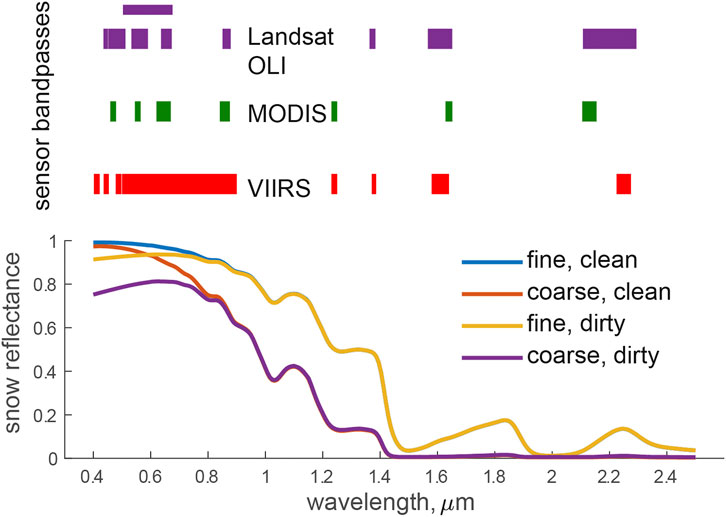
FIGURE 1. Spectral sampling differences between OLI, MODIS, and VIIRS shown as sensor bandpasses plotted with snow spectra for fine and coarse snow with and without light absorbing particles.
The Moderate-resolution Imaging Spectroradiometer (MODIS, Justice et al., 1998) and the Visible Infrared Imaging Spectrometer Suite (VIIRS, Justice et al., 2013) collect data at spatial resolutions of 250 m to 1 km depending on the instrument band. The gridded Level 2 surface reflectance products are provided at 500 m for MODIS and 1 km for VIIRS. At these moderate spatial resolutions, with a daily return interval and global coverage, these sensors have been instrumental in capturing heterogeneous snow cover at the global scale both in complex terrain and at regional to watershed scales (Dozier and Painter, 2004). The MODIS and VIIRS surface reflectance data are also well suited to examine snow cover surface properties in addition to snow cover, such as grain size and light-absorbing impurities (Painter et al., 2012b) that collectively drive the variability in snow albedo.
The snow mapping technique that is applied most commonly to data from multispectral satellites and used worldwide to map snow for products like MOD10A1 (Hall and Riggs, 2007) and the VIIRS Snow Cover product (Justice et al., 2013; Key et al., 2013) uses a computationally simple algorithm developed in the 1980s, when computers were more primitive. This approach, the Normalized Difference Snow Index (NDSI), was developed using band difference ratios (Dozier, 1989) and exploits the fact that snow is bright in the visible and dark in the shortwave-infrared wavelengths. The NDSI algorithm is effective in identifying snow in homogeneous areas where the presence of mixed pixels is low and vegetation is sparse, or at the finest spatial resolutions where most pixels are either entirely snow-covered or bare. However, for snow in rugged terrain, mixed pixels predominate at the MODIS resolution (Selkowitz et al., 2014); and as such, the performance of NDSI is degraded. While the MOD10A1 algorithm produces fractional snow cover (Salomonson and Appel, 2004), the value is from a regression of MODIS NDSI against binary Landsat snow cover maps based on NDSI. Specifically, the 30 m pixels from Landsat are classified as entirely snow-covered or snow-free before aggregation to 500 m for the regression analysis as a target variable. The binary classification of the Landsat data results in a systematic underestimate for snow-covered pixels with less than 50% snow cover and an overestimate for pixels with more than 50% snow cover for MODIS data (Figure 2, in Rittger et al., 2013).
To improve snow mapping for these mixed pixels, the unique spectra of snow, vegetation, and soil/rock combined with multispectral measurements led to the development of spectral un-mixing algorithms that calculate the snow cover fraction (fSCA) of each pixel (Nolin et al., 1993; Rosenthal and Dozier, 1996; Vikhamar and Solberg, 2003; Sirguey et al., 2009; Bair et al., 2020). Spectral unmixing solves simultaneous equations to produce not only fSCA, but also snow surface properties such as grain size and broadband albedo (Painter et al., 2003; Painter et al., 2009). Such algorithms can be applied to reflectance data from any multispectral sensor that includes spectral bands from the visible through shortwave-infrared, and improvements in computational efficiency now enable subpixel snow retrievals from moderate-resolution imagery at the global scale.
While the previous spectral un-mixing algorithms take advantage of all available bands, the algorithm selected by the National Oceanic and Atmospheric Administration (NOAA) for fractional snow cover retrieval was developed for geostationary satellites and uses only visible reflectance (Romanov et al., 2003). NASA’s standard snow cover product from VIIRS relies on the NDSI based method.
The MODIS Snow-Covered Area and Grain-Size algorithm (Painter et al., 2009) produced operationally for the Western United States, the Canadian Rockies and Alaska, High-mountain Asia, the North Pole, and South America demonstrates clear benefits over the standard global operational MODIS Snow Cover Products in mixed pixels and during accumulation and melt (Rittger et al., 2013). MODSCAG data have been used for estimating sub-canopy snow cover (Raleigh et al., 2013; Rittger et al., 2020), light absorbing impurities on snow (Painter et al., 2012b), snow albedo (Bair et al., 2019), persistent ice cover (Painter et al., 2012a), impacts of wildfire on snowmelt (Micheletty et al., 2014), and snow water equivalent (SWE) (Guan et al., 2013; Bair et al., 2016; Rittger et al., 2016). It has also been used for evaluating climate models (Wrzesien et al., 2015; Minder et al., 2016); assimilating data into regional-scale climate models (Oaida et al., 2019); and validating global to regional scale models to better understand regional dust and carbon impacts on snowmelt (Sarangi et al., 2019; Sarangi et al., 2020).
In this study, we use high-resolution fractional snow cover maps, derived from the Landsat 8 Operational Land Imager (OLI) using spectral mixture analysis, to 1) re-evaluate MODSCAG fractional snow cover maps and 2) provide the first evaluation of VIIRSCAG maps over the challenging terrain in High Mountain Asia. The evaluation was conducted using 30 Landsat 8 OLI scenes, spatially spanning two MODIS/VIIRS tiles in the sinusoidal grid in the Himalaya. For the evaluation, we use binary metrics precision, recall, and F-score and fractional metrics mean difference, median difference, and RMSE. Landsat 8 OLI images in 2013 were selected late in the melt and early in the accumulation period, previously shown to be the most challenging times for accurate snow detection. In addition to the evaluation with Landsat 8 OLI, we directly compare snow cover area and snowline elevation from MODSCAG and VIIRSCAG for a more temporally complete dataset over the years of 2012–2015.
The initial validation of MODSCAG and its comparison to widely used snow cover maps from MOD10A1 (Rittger et al., 2013) used Landsat 5 Thematic Mapper (TM) and Landsat 7 Enhanced Thematic Mapper Plus (ETM+) images from Colorado, California, and the Himalaya to understand errors in retrievals from various snow regimes. Rittger et al. (2013) found that MODSCAG RMSE was highest and the probability of detection, also known as recall, was lowest in the Himalaya, which suggested snow identification was more difficult in that region, possibly because of steeper terrain relative to other validation sites in Colorado and California. In addition, this previous work found the highest errors in all regions early in the accumulation season, important for recreation such as skiing, and late in the melt season, when river forecasts are often in error (Dozier, 2011).
For this study, we considered the spatial extent of the Himalayan region to include parts of the Amu Darya, Indus, and Ganges River basins shown in Figure 2. We searched the USGS database of Landsat 8 OLI imagery in 2013 for all images with cloud cover less than 10% in april to July (melt season) and September–November (early accumulation season). We then visually inspected all images and removed those with any cloud cover. The result was a set of 30 images from 17 unique Landsat Worldwide Reference System 2 (WRS2) path/rows covering diverse regions of the Himalaya. This list of images along with the scene-specific validation statistics listed in the previous section is detailed in Supplementary Table S1 of the Supplementary Materials. We selected MODIS and VIIRS images within ± 3 days with the smallest satellite view zenith angles corresponding to nadir viewing Landsat 8 OLI images.
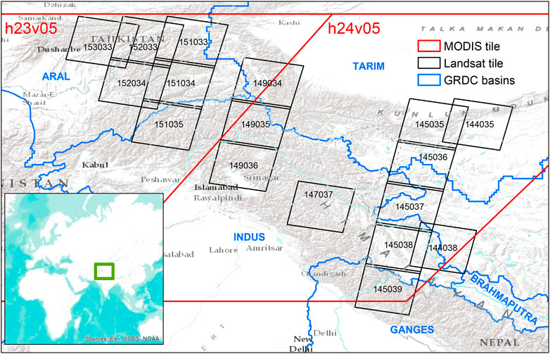
FIGURE 2. The two MODIS tiles and seventeen distinct Landsat tiles used in this study. The comparisons cover parts the Indus, Ganges, and Tarim River basins as well as the Amu Darya River basin (not labeled) in the southern portion of the Aral River basin as provided by the Global Runoff Data Cetner.
The terrain of this study area provides a challenging environment for both MODIS and VIIRS, possibly more challenging for VIIRS because of the coarser spatial resolution relative to MODIS. The climatic characteristics of this domain vary from west to east with westerlies driving much of the precipitation in the Amu Darya and Western Indus, while the monsoon also affects the Eastern Indus and Ganges River basins.
MODIS was launched on both the Terra platform in December 1999 and on the Aqua platform in May 2002. Both Terra and Aqua provide global daily coverage of the earth’s surface with equatorial crossings at 10:30 and 13:30. VIIRS, aboard Suomi National Polar-orbiting Partnership (Suomi NPP), was launched in October 2011 to provide data continuity with long-term data records from NASA’s Earth Observing System and the planned Joint Polar Satellite System (JPSS) instruments (Cao et al., 2013). With near-global daily coverage, moderate resolution retrievals at 11 spectral bands (Figure 1), and a 13:30 overpass time, Suomi NPP VIIRS provides similar information to that from MODIS for snow cover retrievals.
While the daily Aqua overpass aligns temporally with Suomi NPP overpass, the mid-morning MODIS retrievals from Terra are generally preferred for snow retrieval due to cloud-cover considerations. The MODIS instrument aboard Aqua suffered from loss of 75% of its detectors for Band 6 shortly after launch (Gladkova et al., 2012). MODIS Band 6 observes radiances in the spectral range of 1.628–1.652 µm, which is a key bandwidth for common snow retrieval algorithms as shown in Figure 1. Robust discrimination between cloud and snow cover can be challenging (Dietz et al., 2012; Stillinger et al., 2019; White et al., 2020); and as such, we have visually selected clear-sky scenes for this study.
Pixel distortion created by the combination of MODIS scan geometry and the earth’s curvature causes edge-of-scan pixels in MODIS surface reflectance data to be collected from an area nearly 10 times the size of those viewed from nadir (Dozier et al., 2008). Therefore, off-nadir observations image different (larger) areas on the ground than nadir views especially in topographically complex terrain where the view azimuth offsets the direction of pixel elongation (Rittger et al., 2020). To address this shortcoming, the VIIRS instrument uses de-aggregation of sub-pixels at wide scan angles (>32°, Cao et al., 2013) to sample at a more constant spatial resolution in the cross-track direction. This technique reduces edge-of-scan distortion in VIIRS surface reflectance data (Schueler et al., 2013) and, in turn, distortion in representation of perceived snow cover area at the edge of the swath. Because future JPSS missions plan to carry VIIRS optical instrumentation and MODIS’s end-of-life is approaching, the future of continued global fractional snow cover observations will hinge on VIIRS-based retrievals.
For this study, the MODIS inputs used were MOD09GA L2G Surface Reflectance 500 m SIN grid from Collection 5 that are provided by the Land Processes DAAC (lpdaac.usgs.gov). We used Collection 5 instead of the more recent Collection 6 MODIS products to allow direct comparison with previous evaluations of MODSCAG (Rittger et al., 2013). Degradation of visible and near-infrared bands in Collection 5 has been shown to impact long-term trends in geophysical variables, yet the impact is small in an absolute sense (Table 1, in Lyapustin et al., 2014) and below the stated accuracy of MODIS products. The errors in this paper for Collection 5 can be considered a high estimate relative to those if we had used Collection 6. The VIIRS inputs used were the early release products DSRF1KD L2GD Surface Reflectance 1 km SIN grid and DGA1KD L2GD Geolocation Angles 1 km SIN grid from Collection 3110, provided by the Level-1 and Atmosphere Archive and Distribution System (LAADS).
While the VIIRS moderate resolution data are being resolved to 750 m in the native grid projection, the Level 2 gridded products are distributed at 1 km spatial resolution on the MODIS Sinusoidal Tile Grid for consistency with the 500 m MODIS archive. Consequently, the spatial resolution of our snow cover products derived from VIIRS are at 1 km. These surface reflectance products are likely consistent with those used to develop the snow retrieval algorithms for the Standard VIIRS Snow Products, (Key et al., 2013), although these inaugural studies do not explicitly state the data products used. However, since our analysis, Collection 3110 has been replaced by the newer VNP09GA Version 1 Surface Reflectance products. A comparison of the DSRF1KD and VNP09GA surface reflectance products shows minor differences in spectral reflectance over snow (Supplementary Figure S1).
Fractional snow cover and grain size maps are derived from MODIS and VIIRS surface reflectance inputs using the Snow Cover and Grain Size (SCAG) algorithm (Painter et al., 2003; Painter et al., 2009). The algorithm disaggregates pixel-averaged surface reflectance into a group of individual land surface components using a combination of reflectance spectra from pure spectral end member libraries. Commonly known as spectral mixture analysis, the SCAG algorithm is based on a set of simultaneous linear equations that are solved for these individual components (Roberts et al., 1998).
Fi is the fraction of endmember i; Rλ,i is the hemispherical directional reflectance factor (HDRF, Schaepman-Strub et al., 2006) of endmember i at wavelength λ; and ελ is a residual error. We assume a linear combination of reflectances using this method, which is appropriate above timberline where the surface is planar. Below timberline, there are nonlinear interactions with the canopy; however, we include canopy-level vegetation endmembers in the SCAG spectral library that represent multiple scattering and allow the linear assumption. The spectral library contains 109 snow (of varying grain size), 3 ice, 20 vegetation, and 17 rock spectra that were measured in situ (Painter et al., 2003; Painter et al., 2009) and allows for changes in snow spectra with viewing angle. The snow spectral HDRF come from radiative transfer modeling, constrained by snow grain size (10–1100 μm by 10 μm) and solar zenith angle by 15 degree increments (Painter et al., 2003; Painter et al., 2009).
The SCAG model is run iteratively; and with each set of Fi and Rλ,i, we estimate the RMSE as the difference between the modeled and observed pixel-averaged reflectance. SCAG chooses the model with the lowest RMSE that provides estimates of the snow cover fraction, vegetation fraction, and bare soil or rock fraction. Fractional snow cover and other endmembers are normalized by the spectral fraction of photometric shade to account for topographic effects on irradiance. These model runs are constrained to endmember fractions in the range of −0.01–1.01 with an overall RMSE <2.5%, with no three spectrally consecutive residuals exceeding 2.5%. For pixels that do not meet these constraints, a second set of model runs is completed using looser constraints. SCAG selects the model with the fewest endmembers and the smallest RMSE. The selected endmember for snow (where it exists) has an associated grain size in the spectral library, which allows for snow grain size mapping. Whereas this grain size can be converted to a clean snow albedo or combined with impurities to estimate the true snow albedo (Wiscombe and Warren, 1980; Painter et al., 2009), this step is outside the scope of the work presented here. Historically, albedo from snow grain sizes derived with SCAG have been combined with dust impacts on albedo estimated from a separate algorithm (Painter et al., 2012b), however, recent work shows that these variables can be solved for simultaneously (Bair et al., 2020).
The SCAG products used in this study are the fractional snow cover area (fSCA) maps. To account for the spectral differences between MODIS and VIIRS (Figure 1), the high resolution spectral libraries (Painter and Dozier, 2004) were resampled to the VIIRS spectral bands using the relative spectral response data available from the Center for Satellite Applications and Research JPSS website.
We use surface reflectance from USGS Landsat 8 OLI in this study. Landsat 5 TM and Landsat 7 ETM+ have been used to evaluate snow cover products in the past, including those from MODIS (Salomonson and Appel, 2004; Dozier et al., 2008; Painter et al., 2009; Bormann et al., 2012; Rittger et al., 2013; Metsämäki et al., 2015; Yang et al., 2015). TM and ETM+ sensors were designed for observing fine radiometric detail in dark ocean water and when compressed into an 8-bit data stream, result in saturation of the sensor over snow in bands 1, 2, and 3 (Dozier, 1989; Duguay and Ledrew, 1992).
The more snow cover, the brighter the surface at visible wavelengths, and the more likely the sensor will become saturated. When saturation of the sensor occurs, the observed surface reflectance values are lower than the true reflectance. A complicating factor is the use of cubic convolution instead of nearest neighbor processing the USGS uses to resample Landsat data that can merge values from saturated pixels and unsaturated pixels making it more difficult to identify affected pixels.
For spectral mixture analysis, the use of the saturated values would introduce erroneously low reflectance values leading to an underestimation of fSCA. Therefore, when only one or two of the visible bands are saturated, spectral mixture analysis of TM and ETM+ data uses the remainder of the bands to produce the fSCA model output. When all three visible bands are saturated there is insufficient information to apply spectral mixture analysis. Previous work assumed that pixels saturated in all three visible bands were fully snow cover (Painter et al., 2009; Rittger et al., 2013), however, it is possible that they were not.
For this reason, the Landsat 5 TM and Landsat 7 ETM+ are imperfect sources of validation data leading to a systematic positive bias in fSCA from Landsat. The previous evaluation of MODSCAG using these Landsat fSCA estimates as “truth” found a mean bias of −5.2% over four regions and −7.6% in the Himalayan region (Rittger et al., 2013). In this paper, we assess the number of pixels with saturation in previous comparisons to MODIS snow maps. NDSI and regression-based approaches (Hall et al., 2002; Salomonson and Appel, 2004; 2006) that assume accurate Landsat snow cover maps for validation and calibration do not appear to account for this issue, and the standard NASA global-fractional snow products still use regression equations based on saturated sensors.
In contrast to the 8-bit data stream from TM and ETM+, the optical sensor aboard Landsat 8 OLI, uses a 12-bit data stream that allows it to see the darkest ocean to the brightest snow without saturation, allowing the spectral mixture analysis to use all bands for even the brightest pixels. The higher accuracy of Landsat 8 data provide the opportunity to update the evaluation of MODSCAG fractional snow cover maps and contrast it with the first evaluation of VIIRSCAG performance.
We use a set of binary metrics previously used to evaluate MODIS snow cover maps (Rittger et al., 2013) to facilitate comparison to the previous studies. Assuming Landsat 8 snow cover maps to be the “truth”, we classify pixels into four possible outcomes: true positive (TP), true negative (TN), false positive (FP), and false negative (FN). We calculate the four outcomes for both MODIS and VIIRS snow maps and consider pixels <15% to be snow-free, again for consistency with previous studies. Common measures of a classification algorithm’s performance are calculated using the four outcomes:
We abstain from using the accuracy calculation (Eq. 4) because of the overwhelming number of TN pixels included when analyzing full Landsat scenes, which contain large snow-free areas. We find the F score to be the single most useful metric as it balances Precision and Recall, penalizing both missing snow and falsely identified bare areas as snow, while excluding extensive snow-free areas (Wilks, 2006).
We use mean difference, median difference, and RMSE to evaluate performance of the MODIS and VIIRS fractional snow cover maps. We exclude TN occurrences from the RMSE calculation because large snow-free areas, especially in the summer, can result in very small errors (Rittger et al., 2013). Previous studies (Hall et al., 2002; Salomonson and Appel, 2004, 2006; Painter et al., 2009) did include those in the error statistics, therefore yielding lower RMSE values when compared to this study. The RMSE is defined as:
where
We use mean absolute error (MAE) to quantify the discrepancy between the snow fraction for MODIS
We use Landsat 8 OLI data employing the SCAG algorithm to compare with the coarser maps from both MODIS and VIIRS. After mapping fractional snow cover at 30 m spatial resolution, we coarsen the data by identifying the subset of Landsat pixels within each MODIS or VIIRS pixel (∼256 values) and then averaging those values. Similar to previous MODSCAG validation (Rittger et al., 2013), we find that coarsening MODIS from 500 m to 2 km significantly improves both the binary and fractional statistics, indicating a MODIS geolocation error between 1 and 2 pixels as found in other studies (Wolfe et al., 2002). Similarly, we find the same reduction in errors when coarsening the VIIRS data from 1–4 km. We isolate the errors from the SCAG algorithm by performing the analysis at these coarser spatial resolutions.
In this section we briefly discuss the impact of saturation on 30 m snow maps from from Landsat 5 TM and Landsat 7 ETM+. We then compare the binary and fractional statistics for snow maps in the melt and early accumulation periods from MODIS and VIIRS with that of Landsat 8 OLI and discuss the improved snow detection capability relative to Landsat 5 TM and Landsat 7 ETM+.
Rittger et al. (2013) used 25 Himalayan images for validation of MODSCAG with three images from September, fifteen from October, and seven from November. The September through October dates occurred after the equinox when the Sun is lower in the sky and saturation is less likely because of lower incoming shortwave radiation. Figure 3 shows the percent of snow-covered pixels saturated in three band combinations for the 25 images. 28% of the pixels were saturated in all visible bands (1, 2, & 3), and were assumed to be fully snow covered as previously described above in Landsat TM and ETM+. Individually, band 1 saturates most frequently followed by band 3 and then band 2. Overall, 2% of the snow-covered pixels are saturated in band 1 only (not 2 & 3), and 4% of the pixels are saturated in bands 1 & 3 (not 2). This new study uses Landsat 8 OLI which does not saturate, and includes May (n = 9), June (n = 5), September (n = 5), and October (n = 11) of 2013.
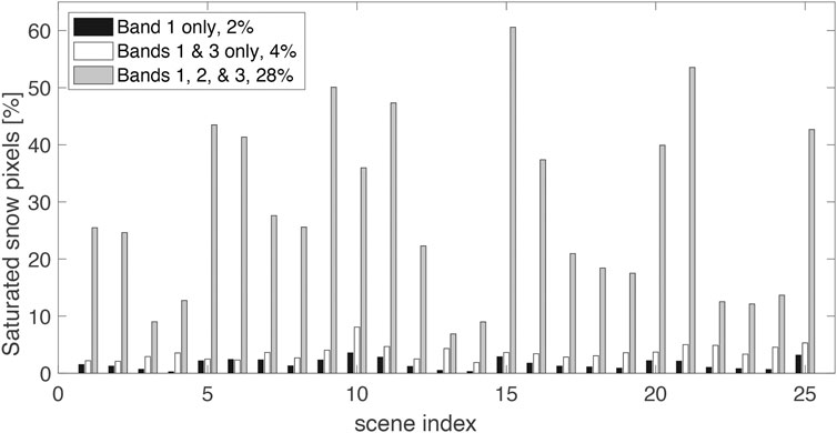
FIGURE 3. Percent of snow-covered pixels saturated in any of the Landsat TM and ETM+ visible channels (bands 1, 2, and 3). The x axis is related to the Himalayan scenes analyzed in Rittger et al., (2013).
The first column in Figure 4 shows the false color Landsat 8 OLI image at 30 m resolution for five dates in the Pamir-Alay mountain system, which runs through Tajikistan, Kyrgyzstan, and Uzbekistan. The Landsat WRS-2 path/row is 153/033, i.e. the Western most region in this study (Figure 2). This region is relatively cloud-free compared to regions to the East and provides the most cloud free images in this study. The second column in Figure 4 shows the fractional snow cover maps for the five image dates. These 30 m snow maps show that most pixels are nearly fully snow covered (white) while there are fewer partially covered snow pixels (blue). When coarsened to 500 m shown in the third column in Figure 4, the fractional snow cover increases as fully snow-covered pixels are aggregated with snow-free pixels, especially near the snowline. The fourth and fifth column in Figure 4, show the fractional snow cover maps at native resolution from MODIS and VIIRS, respectively. Visually, images appear similar from all three sensors indicating agreement.
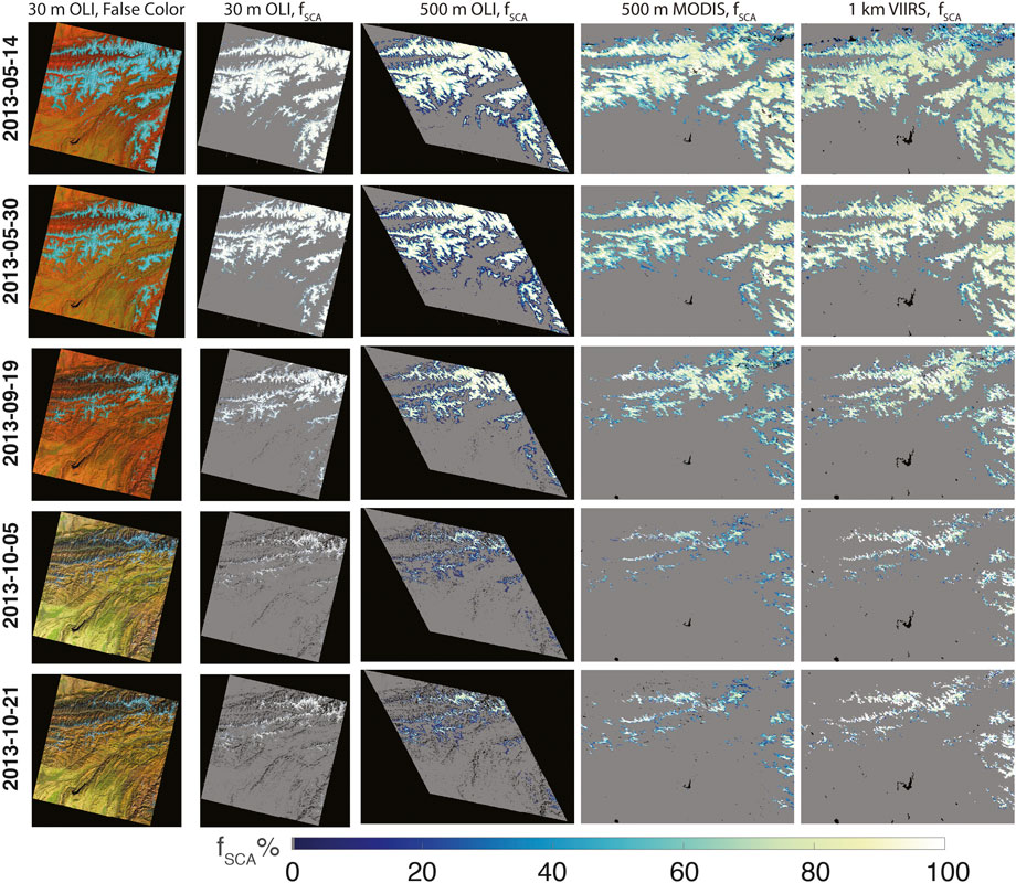
FIGURE 4. Column 1: 30 m Landsat 8 OLI false color using bands 6, 4, and 2 in Universal Transverse Mercator projection zone 42, Column 2: 30 m Landsat 8 OLI fractional snow cover in Universal Transverse Mercator projection zone 42. Column 3: 30 m Landsat 8 OLI fractional snow cover resampled to 500 m in sinusoidal projection, Column 4: 500 m MODIS fractional snow cover in sinusoidal projection, Column 5: 1 km VIIRS fractional snow cover in sinusoidal projection. All fSCA images use the same color scale.
The binary statistics used for comparison of the Landsat 8 OLI snow maps with the snow maps from MODIS and VIIRS are defined in Eqs. 2, 3, 5. Table 1 shows the summary of binary statistics which include the mean, minimum, maximum, and standard deviation for the 30 image comparisons as well as statistics from the previous study. The scene based binary statistics for each of the 30 dates for both MODIS and VIIRS are included in Supplementary Table S1.
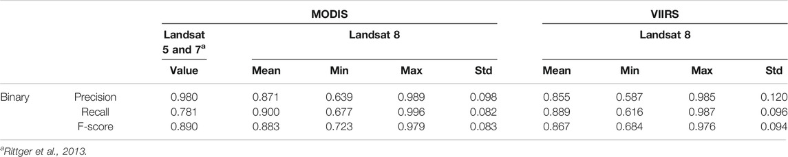
TABLE 1. Summary of binary statistics comparing MODIS and VIIRS fSCA to Landsat fSCA.
The maximum snow cover in the Hindu-Kush Himalayan region occurs in February to March (Figure 3, Armstrong et al., 2019), while minimum snow and ice cover usually occurs in October (Painter et al., 2012a). Therefore, our study covers a period during melt (April–June) and during the minimum and beginning of accumulation (September–November). Figure 5 shows the binary statistics within these time periods and are labeled as Melt Season and Accumulation Season.
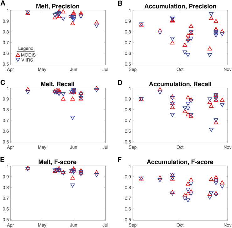
FIGURE 5. Binary metrics for MODIS (red) and VIIRS (blue) images in the Melt Season (column 1) and Accumulation Season (column 2). (A) Melt Season, precision. (B) Accumulation Season, precision. (C) Melt Season, recall. (D) Accumulation Season, recall. (E) Melt Season, F-score. (F) Accumulation Season, F-score.
Precision, which indicates the number of true positives relative to all positives was 0.871 and 0.855 for MODIS and VIIRS, respectively. For MODIS, precision was lower than previously reported; but previous work included midwinter periods where there is much more snow and high values for precision are easier to achieve. Figures 5A,B show the precision during the Melt Season and Accumulation Season, respectively. During Melt Season, a high precision is maintained, while during Accumulation Season there is more scatter with values as low as ∼0.6. Right before accumulation, at the minimum snow cover, precision is a bit higher.
Recall (i.e., the probability of detection) for MODIS and VIIRS was 0.900 and 0.889, respectively. This is considerably higher than previous estimates for MODIS, and is plotted for the Melt Season and Accumulation Season in Figures 5C,D, respectively. Recall during melt is very high for both MODIS and VIIRS except for one outlier on May 31st with a recall of 0.728, which is possibly due to unwanted cloud interference given the otherwise high accuracy across other dates. Similar to precision, recall is lower during early accumulation.
The F-score, which balances precision and recall, was 0.890 and 0.867 for MODIS and VIIRS, respectively. This value was nearly the same in the previous study for MODIS. As shown in Figures 5E,F, the F-score is higher in the Melt Season than the Accumulation Season as also seen in previous work. Compared to previous work, precision is lower but recall is higher, resulting in a similar overall F-score as assessed by binary statistics.
Table 2 shows the summary (mean, minimum, maximum, and standard deviation) of fractional statistics described in previously in Evaluation Metrics. These fractional statistics on each date for both MODIS and VIIRS are included in Supplementary Table S1. The fractional metrics for the Melt Season period are shown in Figure 6A and for the Accumulation Season period in Figure 6B. The mean and median difference during the Melt Season period are nearly all less than 0.01 when averaged for all 30 images (Table 2) for both MODIS and VIIRS fSCA. Figures 6A,B show the mean, whereas Figures 6C,D show the median over time. Median errors are smaller than mean errors, indicating a few larger errors as opposed to a more normally distributed set of errors. This also indicates that the accumulation season has more large errors than the melt season, which is also seen in the RMSE errors plotted in Figure 6F and compared to Figure 6E. The RMSE, like all the other statistics, was lower during the melt season and higher during the minimum and the start of accumulation.
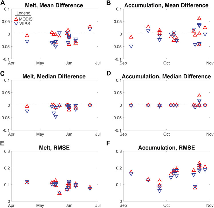
FIGURE 6. Fractional metrics for MODIS (red) and VIIRS (blue) images in the Melt Season (column 1) and Accumulation Season (column 2). (A) Melt Season, mean difference. (B) Accumulation Season, mean difference. (C) Melt Season, median difference. (D) Accumulation Season, median difference. (E) Melt Season, RMSE. (F) Accumulation Season, RMSE.
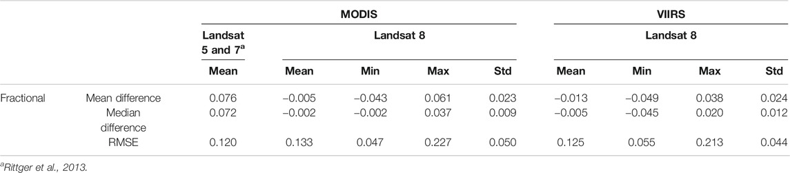
TABLE 2. Summary of fractional statistics comparing MODIS and VIIRS fSCA to Landsat fSCA.
We compare the distribution of fractional snow cover values from MODIS and VIIRS to each other and examine differences across elevation, slope, and aspect gradients. We present a comparison of two common metrics–total snow-covered area and regional snowline elevations–directly between MODIS and VIIRS to demonstrate continuity between the instruments.
A direct comparison of snow-covered area from the MODIS and VIIRS fSCA products (Figure 4, columns 4 and 5, respectively) on the evaluation dates (Supplementary Table S1) returns a MAE (Eq. 7) of 10.5% with an mean difference of +3.2%. When we expand the evaluation to the full set of coincident scenes for the period 2012–2015 for the two tiles shown in Figure 2 and limit to clear sky dates (<2% cloud), we find the MAE in snow cover area remains relatively consistent at 10.8%, and VIIRS tends to underestimate snow cover area by an average of −4.3%, indicating that VIIRS generally reports slightly less snow cover area than MODIS. The switch from positive VIIRS bias to negative VIIRS bias when the evaluation is expanded from 30 dates to three complete years is a reflection of the change in distribution of the months and seasons represented in the two samples. We consider the underestimation from VIIRS relative to MODIS of −4.3% to be more representative of overall performance. Note that these values are a measure of agreement between MODIS and VIIRS snow cover products rather than an evaluation with Landsat 8 OLI maps (Table 1; Figures 5, 6), hence these values differ from those presented earlier.
A comparison of the frequency distribution of fSCA values between the two sensors in Figure 7 shows distributions and the overall median fSCA values to be very similar, 70% for MODSCAG and 71% for VIIRSCAG. These statistics and frequency distributions are consistent when evaluated for each tile individually, with median fSCA values of 67% and 70% for MODIS and 68% and 69% for VIIRS for the h23v05 and h24v05 tiles, respectively. Further analysis of the frequency distribution of fSCA values reveals that, overall, MODIS products find ∼7% purer snow-covered pixels than VIIRS with MODSCAG having more pixels covered (88%–100%), visible as taller red bars in Figure 7. The VIIRS products return more snow covered pixels (50%–88%), visible as taller blue bars in Figure 7.
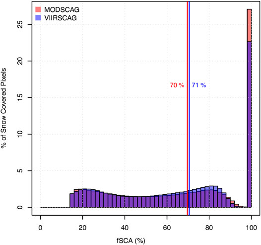
FIGURE 7. fSCA for MODIS (500 m) and VIIRS (1 km) for the full period of record (2012–2015) across both h23v05 and h24v05 tiles combined. The mean fSCA values are for each sensor (70% for MODSCAG and 71% for VIIRSCAG shown in red and blue respectively) are shown with a vertical line. Only clear sky days were included (scene cloud <0.8%).
The expected frequency distribution shift is likely a reflection of the differences in spatial resolution of the gridded reflectance data used as inputs to the snow retrieval algorithm; there are likely more mixed pixels at 1 km VIIRS resolution than at the 500 m MODIS resolution.
The two MODIS tiles (Figure 2) are exceptionally clear on September 18, 2013 (<0.8% clouds). Figures 8A,B show the MODIS and VIIRS fSCA, respectively, along with spatial fSCA differences between the two snow cover products in Figure 8C. The comparison between Figures 8A,B shows good agreement, with a higher abundance of high fSCA values in the MODIS data leading to negative differences in Figure 8C, which are spatially correlated with the 88%–100% fSCA pixels in the MODIS data (see Figure 7). Figure 8D shows the vegetation type (Arino et al., 2010) while Figures 8E,F show the elevation and slope. These data are used for the topographic analysis shown in Figures 9, 10.
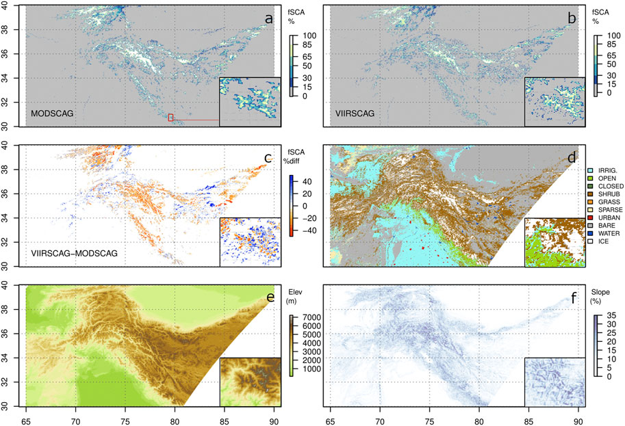
FIGURE 8. Comparison of (A) MODIS and (B) VIIRS-derived fSCA for two MODIS tiles used in this study (Figure 2), difference in fSCA(C). For the analysis shown in Figures 9 and 10: Globcover land cover class (D), elevation (E), and terrain slope (F). The inset shows a zoom region over a 111 × 78 km region as marked by the red viewport in panel (A). The satellite view zenith for MODIS was twice that of VIIRS in these data.
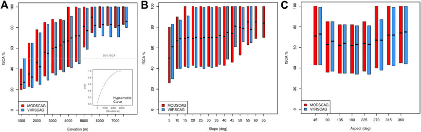
FIGURE 9. Similarities between MODIS and VIIRS fSCA retrievals across (A) elevation, (B) slope, and (C) aspect gradients for the full timeseries 2012 to 2015 for tile h23v05. The hypsometric curve generated from the DEM for the entire tile is shown as an inset.
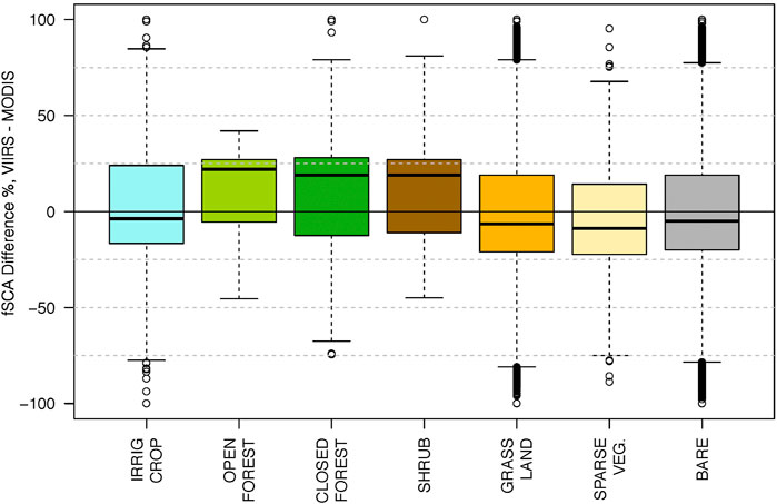
FIGURE 10. Summary of differences in fSCA (VIIRS-MODIS) over full HMA region on September 18, 2013 summarized in each GlobCover land cover class, where positive differences indicate VIIRS fSCA > MODIS fSCA. The high bias in vegetated areas (open forest and closed forest classes) are likely due to differences in view angle with the MODIS view angle for this day twice that of VIIRS. Figure 9B inset (VIIRS fSCA) shows more fractional snow cover than Figure 9A inset (MODIS fSCA) in open forest visible in Figure 9D supporting this conclusion.
The fSCA retrievals for both sensors show similar performance across elevation, slope, and aspect gradients in tile h23v05 (Figures 9A–C), where we also compared Landsat 8 OLI in Results. The performance between the sensors is nearly the same for tile h24v05 (not shown), although the distribution of snow cover fraction with elevation is modulated by a more variable hypsometric curve along with monsoonal climates that occur in the eastern portion of the Himalaya.
Figure 10 shows fSCA compared across two MODIS tiles for September 18, 2013 segmented by vegetation types (Figure 8D). We see larger fSCA values (up to 23%) retrieved from VIIRS in vegetated areas. However, in this region, there are very few pixels classified as “open forest” or “closed forest” relative to other land surfaces resulting in the relatively similar comparison shown in Figure 9. Therefore, the impact on total snow cover is relatively small. An analysis of the ancillary data shows that over the vegetated regions (open forest, closed forest, and shrub), sensor view zenith for MODIS is 44.6° and 45.9°, whereas for VIIRS they are 23.1° and 25.5°, respectively, for the two tiles. The larger view zenith for MODIS relative to VIIRS explains the higher estimate of snow cover from VIIRS. The analysis of differences related to view zenith is outside the scope of this paper and of interest for further research but is described in Evaluation Metrics of Dozier et al. (2008) and also in Rittger et al. (2020).
With respect to consistency between the MODIS and VIIRS fractional snow cover products, we compare snow cover area and regional snowline elevation across tile h23v05 at the common resolution of 1 km for 2013 to 2015. We observe a strong correlation between the snow cover area retrievals (R2 = 0.98) and regional snowline elevation estimation (R2 = 0.88) as shown in Figure 11. The strong agreement between MODIS and VIIRS snow cover retrievals supports the continuation and augmentation of existing MODIS timeseries from 2000-present with VIIRS retrievals, as the MODIS instruments reach end of life and the observation record of VIIRS continues forward in time.
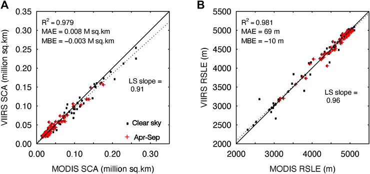
FIGURE 11. Comparison of MODIS and VIIRS-derived total snow cover area (A) and regional snowline elevation (B) for tile h23v05. The panels show data for 2012–2015 period on clear-sky days only i.e. < 2% cloud cover. All clear-sky days are plotted as black squares with the red crosses plotted over the observations from April–September.
An evaluation of new moderate resolution fractional snow cover maps from VIIRS retrievals (VIIRSCAG) in the Himalaya show performance statistics comparable to the more widely evaluated and available MODSCAG products. MODSCAG fractional snow cover maps re-evaluated using snow maps from Landsat 8 OLI do not show the negative bias found in a previous study. The reason for the improvement in MODSCAG performance revealed in this analysis is due to the improved Landsat 8 OLI validation data, more specifically improved sensor technology that avoids saturation in the visible bands and systematic overestimation bias in the validation maps from the assumption of 100% snow cover when bands 1, 2, and 3 were saturated in Landsat TM and ETM+.
MODSCAG snow retrievals were expected to outperform those from VIIRSCAG in the steep terrain of the Himalaya, largely due to the finer spatial resolution of MODIS data. However, despite the coarser native resolution of the gridded products (1 km vs 500 m), VIIRSCAG evaluations produced slightly lower overall RMSE than for MODSCAG, perhaps because of improved representation of pixels toward the edge of the scan. The correlation and similarity in snow elevation and snow-covered area between MODIS and VIIRS observations over a three-year period, along with similar performance when compared to Landsat 8 OLI, show the ability of spectral mixture analysis to perform consistently over a range of spatial resolutions, making it a good candidate for multi-satellite fusion efforts. In addition, the VIIRSCAG snow products appear to be suitable for extending the long-term SCAG timeseries (now at 20 years) well beyond the life of MODIS. Extending this record is important to performing snow cover change evaluation to monitor regional climate change. Future MODSCAG processing will benefit from MODIS Collection 6 surface reflectance products, which may allow processing of Aqua data in addition to Terra.
The datasets presented in this study can be found in online repositories. The names of the repository/repositories and accession number(s) can be found below: (Rittger, 2021).
KR: Conceptualization, Funding acquisition, Methodology, Formal analysis, Data curation, Visualization, Writing–Original Draft, Writing–Review and Editing KB: Conceptualization, Methodology, Formal analysis, Data curation, Visualization, Writing–Original Draft, Writing–Review and Editing EB: Writing–Original Draft, Writing–Review and Editing, Funding acquisition JD: Methodology, Project administration, Funding acquisition, Writing–Original Draft, Writing–Review and Editing TP: Methodology, Software, Project administration, Funding acquisition, Writing–Original Draft, Writing–Review and Editing.
NASA award 80NSSC18K1489; NASA award 80NSSC18K0427; NASA award 80NSSC20K1721; NOAA award NA18OAR4590380.
Authors KB and TP were employed by the company Airborne Snow Observatories Inc.
The remaining authors declare that the research was conducted in the absence of any commercial or financial relationships that could be construed as a potential conflict of interest.
We acknowledge data contributions from the Jet Propulsion Laboratory and continued support from NASA Terrestrial Hydrology for SCAG/DRFS products.
The Supplementary Material for this article can be found online at: https://www.frontiersin.org/articles/10.3389/frsen.2021.647154/full#supplementary-material.
Arino, O., Ramos, J., Kalogirou, V., Defourny, P., and Achad, F. (2010). “GlobCover 2009”, in Proceedings of the ESA Living Planet Symposium, SP-686. Available at: http://due.esrin.esa.int/page_globcover.php.
Armstrong, R. L., Rittger, K., Brodzik, M. J., Racoviteanu, A., Barrett, A. P., Khalsa, S.-J. S., et al. (2019). Runoff from glacier ice and seasonal snow in high asia: separating melt water sources in river flow. Reg. Environ. Change 19, 1249–1261. doi:10.1007/s10113-018-1429-0
Arnell, N. (1999). Climate change and global water resources. Glob. Environ. Change 9 (Suppl. 1), S31–S49. doi:10.1016/S0959-3780(99)00017-5
Bair, E. H., Rittger, K., Davis, R. E., Painter, T. H., and Dozier, J. (2016). Validating reconstruction of snow water equivalent in California's Sierra Nevada using measurements from the NASAAirborne Snow Observatory. Water Resour. Res. 52, 8437–8460. doi:10.1002/2016WR018704
Bair, E. H., Rittger, K., Skiles, S. M., and Dozier, J. (2019). An examination of snow albedo estimates from MODIS and their impact on snow water equivalent reconstruction. Water Resour. Res. 55, 7826–7842. doi:10.1029/2019wr024810
Bair, E. H., Stillinger, T., and Dozier, J. (2020). Snow property inversion from remote sensing (SPIReS): a generalized multispectral unmixing approach with examples from MODIS and Landsat 8 OLI. IEEE Trans. Geosci. Remote Sensing, 1–15. doi:10.1109/TGRS.2020.3040328
Bormann, K. J., Brown, R. D., Derksen, C., and Painter, T. H. (2018). Estimating snow-cover trends from space. Nat. Clim Change 8, 924–928. doi:10.1038/s41558-018-0318-3
Bormann, K. J., McCabe, M. F., and Evans, J. P. (2012). Satellite based observations for seasonal snow cover detection and characterisation in Australia. Remote Sensing Environ. 123, 57–71. doi:10.1016/j.rse.2012.03.003
Cao, C., Xiong, J., Blonski, S., Liu, Q., Uprety, S., Shao, X., et al. (2013). Suomi NPP VIIRS sensor data record verification, validation, and long-term performance monitoring. J. Geophys. Res. Atmos. 118 (20), 664–678. doi:10.1002/2013JD020418
Derksen, C., and Brown, R. (2012). Spring snow cover extent reductions in the 2008-2012 period exceeding climate model projections. Geophys. Res. Lett. 39, L19504. doi:10.1029/2012gl053387
Dettinger, M. D., and Cayan, D. R. (1995). Large-scale Atmospheric forcing of recent trends toward early snowmelt Runoff in California. J. Clim. 8, 606–623. doi:10.1175/1520-0442(1995)008<0606:lsafor>2.0.co;2
Dietz, A. J., Kuenzer, C., Gessner, U., and Dech, S. (2012). Remote sensing of snow - a review of available methods. Int. J. Remote Sensing 33, 4094–4134. doi:10.1080/01431161.2011.640964
Dozier, J. (2011). Mountain hydrology, snow color, and the fourth paradigm. Eos Trans. AGU 92, 373–374. doi:10.1029/2011eo430001
Dozier, J., and Painter, T. H. (2004). Multispectral and hyperspectral remote sensing of alpine snow properties. Annu. Rev. Earth Planet. Sci. 32, 465–494. doi:10.1146/annurev.earth.32.101802.120404
Dozier, J., Painter, T. H., Rittger, K., and Frew, J. E. (2008). Time-space continuity of daily maps of fractional snow cover and albedo from MODIS. Adv. Water Resour. 31, 1515–1526. doi:10.1016/j.advwatres.2008.08.011
Dozier, J. (1989). Spectral signature of alpine snow cover from the Landsat Thematic Mapper. Remote Sensing Environ. 28, 9–22. doi:10.1016/0034-4257(89)90101-6
Duguay, C. R., and Ledrew, E. F. (1992). Estimating surface reflectance and albedo from Landsat-5 Thematic Mapper over rugged terrain. Photogrammetric Eng. Remote Sensing 58, 551–558.
Gladkova, I., Grossberg, M. D., Shahriar, F., Bonev, G., and Romanov, P. (2012). Quantitative restoration for MODIS band 6 on Aqua. IEEE Trans. Geosci. Remote Sensing 50, 2409–2416. doi:10.1109/TGRS.2011.2173499
Guan, B., Molotch, N. P., Waliser, D. E., Jepsen, S. M., Painter, T. H., and Dozier, J. (2013). Snow water equivalent in the Sierra Nevada: blending snow sensor observations with snowmelt model simulations. Water Resour. Res. 49, 5029–5046. doi:10.1002/wrcr.20387
Hall, D. K., and Riggs, G. A. (2007). Accuracy assessment of the MODIS snow products. Hydrol. Process. 21, 1534–1547. doi:10.1002/hyp.6715
Hall, D. K., Riggs, G. A., Salomonson, V. V., DiGirolamo, N. E., and Bayr, K. J. (2002). MODIS snow-cover products. Remote Sensing Environ. 83, 181–194. doi:10.1016/S0034-4257(02)00095-0
Justice, C. O., Román, M. O., Csiszar, I., Vermote, E. F., Wolfe, R. E., Hook, S. J., et al. (2013). Land and cryosphere products from Suomi NPP VIIRS: overview and status. J. Geophys. Res. Atmos. 118, 9753–9765. doi:10.1002/jgrd.50771
Justice, C. O., Vermote, E., Townshend, J. R. G., Defries, R., Roy, D. P., Hall, D. K., et al. (1998). The Moderate Resolution Imaging Spectroradiometer (MODIS): land remote sensing for global change research. IEEE Trans. Geosci. Remote Sensing 36, 1228–1249. doi:10.1109/36.701075
Key, J. R., Mahoney, R., Liu, Y., Romanov, P., Tschudi, M., Appel, I., et al. (2013). Snow and ice products from Suomi NPP VIIRS. J. Geophys. Res. Atmos. 118 (12), 816–830. doi:10.1002/2013jd020459
Lyapustin, A., Wang, Y., Xiong, X., Meister, G., Platnick, S., Levy, R., et al. (2014). Scientific impact of MODIS C5 calibration degradation and C6+ improvements. Atmos. Meas. Tech. 7, 4353–4365. doi:10.5194/amt-7-4353-2014
Metsämäki, S., Pulliainen, J., Salminen, M., Luojus, K., Wiesmann, A., Solberg, R., et al. (2015). Introduction to GlobSnow snow extent products with considerations for accuracy assessment. Remote Sensing Environ. 156, 96–108. doi:10.1016/j.rse.2014.09.018
Micheletty, P. D., Kinoshita, A. M., and Hogue, T. S. (2014). Application of MODIS snow cover products: wildfire impacts on snow and melt in the Sierra Nevada. Hydrol. Earth Syst. Sci. Discuss. 11, 7513–7549. doi:10.5194/hessd-11-7513-2014
Minder, J. R., Letcher, T. W., and Skiles, S. M. (2016). An evaluation of high-resolution regional climate model simulations of snow cover and albedo over the Rocky Mountains, with implications for the simulated snow-albedo feedback. J. Geophys. Res. Atmos. 121, 9069–9088. doi:10.1002/2016JD024995
Nolin, A. W., Dozier, J., and Mertes, L. A. K. (1993). Mapping alpine snow using a spectral mixture modeling technique. A. Glaciology. 17, 121–124. doi:10.3189/S0260305500012702
Oaida, C. M., Reager, J. T., Andreadis, K. M., David, C. H., Levoe, S. R., Painter, T. H., et al. (2019). A high-resolution data assimilation framework for snow water equivalent estimation across the western United States and validation with the airborne snow observatory. J. Hydrometeorology 20, 357–378. doi:10.1175/JHM-D-18-0009.1
Painter, T. H., Brodzik, M. J., Racoviteanu, A., and Armstrong, R. (2012a). Automated mapping of Earth's annual minimum exposed snow and ice with MODIS. Geophys. Res. Lett. 39, L20501. doi:10.1029/2012GL053340
Painter, T. H., Bryant, A. C., and Skiles, S. M. (2012b). Radiative forcing by light absorbing impurities in snow from MODIS surface reflectance data. Geophys. Res. Lett. 39, (17):17502. doi:10.1029/2012GL052457
Painter, T. H., and Dozier, J. (2004). Measurements of the hemispherical-directional reflectance of snow at fine spectral and angular resolution. J. Geophys. Res. 109, D18115. doi:10.1029/2003jd004458
Painter, T. H., Dozier, J., Roberts, D. A., Davis, R. E., and Green, R. O. (2003). Retrieval of subpixel snow-covered area and grain size from imaging spectrometer data. Remote Sensing Environ. 85, 64–77. doi:10.1016/s0034-4257(02)00187-6
Painter, T. H., Flanner, M. G., Kaser, G., Marzeion, B., VanCuren, R. A., and Abdalati, W. (2013). End of the little ice age in the alps forced by industrial black carbon. Proc. Natl. Acad. Sci. 110, 15216–15221. doi:10.1073/pnas.1302570110
Painter, T. H., Rittger, K., McKenzie, C., Slaughter, P., Davis, R. E., and Dozier, J. (2009). Retrieval of subpixel snow covered area, grain size, and albedo from MODIS. Remote Sensing Environ. 113, 868–879. doi:10.1016/j.rse.2009.01.001
Raleigh, M. S., Rittger, K., Moore, C. E., Henn, B., Lutz, J. A., and Lundquist, J. D. (2013). Ground-based testing of MODIS fractional snow cover in subalpine meadows and forests of the Sierra Nevada. Remote Sensing Environ. 128, 44–57. doi:10.1016/j.rse.2012.09.016
Rittger, K., Bair, E. H., Kahl, A., and Dozier, J. (2016). Spatial estimates of snow water equivalent from reconstruction. Adv. Water Resour. 94, 345–363. doi:10.1016/j.advwatres.2016.05.015
Rittger, K., Painter, T. H., and Dozier, J. (2013). Assessment of methods for mapping snow cover from MODIS. Adv. Water Resour. 51, 367–380. doi:10.1016/j.advwatres.2012.03.002
Rittger, K., Raleigh, M. S., Dozier, J., Hill, A. F., Lutz, J. A., and Painter, T. H. (2020). Canopy adjustment and improved cloud detection for remotely sensed snow cover mapping. Water Resour. Res. 56, e2019WR024914. doi:10.1029/2019WR024914
Rittger, K. (2021). Snow Cover From Spectral Mixture Analysis Algorithm SCAG: OLI, MODIS, VIIRS. Zenodo. doi:10.5281/zenodo.4733252
Roberts, D. A., Gardner, M., Church, R., Ustin, S., Scheer, G., and Green, R. O. (1998). Mapping chaparral in the santa monica mountains using multiple endmember spectral mixture models. Remote Sensing Environ. 65, 267–279. doi:10.1016/S0034-4257(98)00037-6
Romanov, P., Tarpley, D., Gutman, G., and Carroll, T. (2003). Mapping and monitoring of the snow cover fraction over North America. J. Geophys. Res. 108. doi:10.1029/2002JD003142
Rosenthal, W., and Dozier, J. (1996). Automated mapping of montane snow cover at subpixel resolution from the Landsat Thematic Mapper. Water Resour. Res. 32, 115–130. doi:10.1029/95WR02718
Salomonson, V. V., and Appel, I. (2006). Development of the aqua MODIS NDSI fractional snow cover algorithm and validation results. IEEE Trans. Geosci. Remote Sensing 44, 1747–1756. doi:10.1109/tgrs.2006.876029
Salomonson, V. V., and Appel, I. (2004). Estimating fractional snow cover from MODIS using the normalized difference snow index. Remote Sensing Environ. 89, 351–360. doi:10.1016/j.rse.2003.10.016
Sarangi, C., Qian, Y., Rittger, K., Bormann, K. J., Liu, Y., Wang, H., et al. (2019). Impact of light-absorbing particles on snow albedo darkening and associated radiative forcing over high-mountain Asia: high-resolution WRF-chem modeling and new satellite observations. Atmos. Chem. Phys. 19, 7105–7128. doi:10.5194/acp-19-7105-2019
Sarangi, C., Qian, Y., Rittger, K., Ruby Leung, L., Chand, D., Bormann, K. J., et al. (2020). Dust dominates high-altitude snow darkening and melt over high-mountain Asia. Nat. Clim. Chang. 10, 1045–1051. doi:10.1038/s41558-020-00909-3
Schaepman-Strub, G., Schaepman, M. E., Painter, T. H., Dangel, S., and Martonchik, J. V. (2006). Reflectance quantities in optical remote sensing-definitions and case studies. Remote Sensing Environ. 103, 27–42. doi:10.1016/j.rse.2006.03.002
Schueler, C. F., Lee, T. F., and Miller, S. D. (2013). VIIRS constant spatial-resolution advantages. Int. J. Remote Sensing 34, 5761–5777. doi:10.1080/01431161.2013.796102
Selkowitz, D., Forster, R., and Caldwell, M. (2014). Prevalence of pure versus mixed snow cover pixels across spatial resolutions in alpine environments. Remote Sensing 6, 12478–12508. doi:10.3390/rs61212478
Sirguey, P., Mathieu, R., and Arnaud, Y. (2009). Subpixel monitoring of the seasonal snow cover with MODIS at 250 m spatial resolution in the Southern alps of New Zealand: methodology and accuracy assessment. Remote Sensing Environ. 113, 160–181. doi:10.1016/j.rse.2008.09.008
Stewart, I. T., Cayan, D. R., and Dettinger, M. D. (2005). Changes toward earlier streamflow timing across Western North America. J. Clim. 18, 1136–1155. doi:10.1175/JCLI3321.1
Stillinger, T., Roberts, D. A., Collar, N. M., and Dozier, J. (2019). Cloud masking for Landsat 8 and MODIS Terra over snow‐covered terrain: error analysis and spectral similarity between snow and cloud. Water Resour. Res. 55, 6169–6184. doi:10.1029/2019WR024932
Vikhamar, D., and Solberg, R. (2003). Subpixel mapping of snow cover in forests by optical remote sensing. Remote Sensing Environ. 84, 69–82. doi:10.1016/S0034-4257(02)00098-6
Warren, S. G., and Brandt, R. E. (2008). Optical constants of ice from the ultraviolet to the microwave: a revised compilation. J. Geophys. Res. 113, D14220. doi:10.1029/2007jd009744
White, C. H., Heidinger, A. K., and Ackerman, S. A. (2020). Evaluation of VIIRS neural network cloud detection against current operational cloud masks. Atmos. Meas. Tech. Discuss. 2020, 1–34. doi:10.5194/amt-2020-419
Wilks, D. S. (2006). Statistical methods in the atmospheric sciences. Second ed. Burlington, MA: Elsevier, 628.
Wiscombe, W. J., and Warren, S. G. (1980). A model for the spectral albedo of snow. I: pure snow. J. Atmos. Sci. 37(12), 2712–2733. doi:10.1175/1520-0469(1980)037<2712:AMFTSA>2.0.CO;2
Wolfe, R. E., Nishihama, M., Fleig, A. J., Kuyper, J. A., Roy, D. P., Storey, J. C., et al. (2002). Achieving sub-pixel geolocation accuracy in support of MODIS land science. Remote Sensing Environ. 83, 31–49. doi:10.1016/s0034-4257(02)00085-8
Wrzesien, M. L., Pavelsky, T. M., Kapnick, S. B., Durand, M. T., and Painter, T. H. (2015). Evaluation of snow cover fraction for regional climate simulations in the Sierra Nevada. Int. J. Climatol 35, 2472–2484. doi:10.1002/joc.4136
Yang, J., Jiang, L., Ménard, C. B., Luojus, K., Lemmetyinen, J., and Pulliainen, J. (2015). Evaluation of snow products over the Tibetan Plateau. Hydrol. Process. 29, 3247–3260. doi:10.1002/hyp.10427
Keywords: snow cover, spectral mixture analysis, landsat (OLI), modis, viirs, multispectral imaging
Citation: Rittger K, Bormann KJ, Bair EH, Dozier J and Painter TH (2021) Evaluation of VIIRS and MODIS Snow Cover Fraction in High-Mountain Asia Using Landsat 8 OLI. Front. Remote Sens. 2:647154. doi: 10.3389/frsen.2021.647154
Received: 29 December 2020; Accepted: 31 March 2021;
Published: 10 May 2021.
Edited by:
Soo Chin Liew, National University of Singapore, SingaporeReviewed by:
Qiangqiang Yuan, Wuhan University, ChinaCopyright © 2021 Rittger, Bormann, Bair, Dozier and Painter. This is an open-access article distributed under the terms of the Creative Commons Attribution License (CC BY). The use, distribution or reproduction in other forums is permitted, provided the original author(s) and the copyright owner(s) are credited and that the original publication in this journal is cited, in accordance with accepted academic practice. No use, distribution or reproduction is permitted which does not comply with these terms.
*Correspondence: Karl Rittger, S2FybC5SaXR0Z2VyQGNvbG9yYWRvLmVkdQ==
Disclaimer: All claims expressed in this article are solely those of the authors and do not necessarily represent those of their affiliated organizations, or those of the publisher, the editors and the reviewers. Any product that may be evaluated in this article or claim that may be made by its manufacturer is not guaranteed or endorsed by the publisher.
Research integrity at Frontiers
Learn more about the work of our research integrity team to safeguard the quality of each article we publish.