
94% of researchers rate our articles as excellent or good
Learn more about the work of our research integrity team to safeguard the quality of each article we publish.
Find out more
METHODS article
Front. Remote Sens., 15 February 2021
Sec. Multi- and Hyper-Spectral Imaging
Volume 1 - 2020 | https://doi.org/10.3389/frsen.2020.623678
 Brandon Smith1,2
 Nima Pahlevan1,2*John Schalles3
 Steve Ruberg4Reagan Errera4
 Ronghua Ma5
 Claudia Giardino6
 Mariano Bresciani6Claudio Barbosa7
 Tim Moore8Virginia Fernandez9Krista Alikas10Kersti Kangro10
Retrieval of aquatic biogeochemical variables, such as the near-surface concentration of chlorophyll-a (Chla) in inland and coastal waters via remote observations, has long been regarded as a challenging task. This manuscript applies Mixture Density Networks (MDN) that use the visible spectral bands available by the Operational Land Imager (OLI) aboard Landsat-8 to estimate Chla. We utilize a database of co-located in situ radiometric and Chla measurements (N = 4,354), referred to as Type A data, to train and test an MDN model (MDNA). This algorithm’s performance, having been proven for other satellite missions, is further evaluated against other widely used machine learning models (e.g., support vector machines), as well as other domain-specific solutions (OC3), and shown to offer significant advancements in the field. Our performance assessment using a held-out test data set suggests that a 49% (median) accuracy with near-zero bias can be achieved via the MDNA model, offering improvements of 20 to 100% in retrievals with respect to other models. The sensitivity of the MDNA model and benchmarking methods to uncertainties from atmospheric correction (AC) methods, is further quantified through a semi-global matchup dataset (N = 3,337), referred to as Type B data. To tackle the increased uncertainties, alternative MDN models (MDNB) are developed through various features of the Type B data (e.g., Rayleigh-corrected reflectance spectra
Near-surface concentration of chlorophyll-a (Chla), a proxy for phytoplankton biomass, has been observed and quantified in aquatic ecosystems through optical remote sensing for many years (Clarke et al., 1970; Wezernak et al., 1976; Smith and Baker 1982; Gordon et al., 1983; Bukata et al., 1995). This technique has led to the routine production of Chla distributions for the global oceans for more than two decades. The heritage algorithms have used blue-green band-ratio models to estimate Chla (Gordon et al., 1980; O’Reilly et al., 1998), which are realistic representations of biomass in ecosystems where other constituents, such as detritus and colored dissolved organic matter (CDOM), co-vary with Chla. In optically complex inland and coastal waters however, the color of water is further modulated by the presence of organic and inorganic particles, as well as dissolved matter (Han et al., 1994; Harding et al., 1994) that do not generally co-vary with phytoplankton, rendering retrievals of Chla a far more challenging task (IOCCG 2000). To improve estimates of Chla in these turbid and eutrophic environments, other methods have been developed. For example, spectral bands within the red-edge (RE) region (690–715 nm) (Vos et al., 1986; Mittenzwey et al., 1992), combined with red bands have shown to correlate well with Chla in turbid and/or eutrophic waters (Munday and Zubkoff 1981; Gower et al., 1984; Khorram et al., 1987; Gitelson 1992; Rundquist et al., 1996; Gitelson et al., 2007). The RE observations, however, are not available in the suite of measurements made by heritage missions – such as Landsat—which have provided the longest record of Earth observation from space (Goward et al., 2017).
The Operational Land Imager (OLI) aboard Landsat-8 was launched in February 2013 to continue Landsat’s mission of monitoring Earth systems and capturing changes at relatively high spatial resolution (30 m) (Irons et al., 2012). This mission has offered significant improvements in both data quality and quantity (i.e., both spectral and spatial coverage) over previous heritage instruments (Markham et al., 2014; Pahlevan et al., 2014; Markham et al., 2015). Several methods have been developed to retrieve Chla from the four OLI visible bands (Allan et al., 2015; Watanabe et al., 2015; Concha and Schott 2016; Manuel et al., 2020), yet Chla retrieval methods in inland and coastal waters using traditional approaches are challenged by optical complexity and high dynamic ranges where water types can range anywhere from very clear to highly turbid and eutrophic (Spyrakos et al., 2018). It is, therefore, critical to continue to formulate novel methodologies that enable the production of viable Chla products from Landsat-8 data for global scientific studies and applications (Snyder et al., 2017). Pahlevan et al. (2020) successfully applied Mixture Density Networks (MDNs) – a class of neural networks that estimates multimodal Gaussian distributions over a range of solutions – to Sentinel-2 and Sentinel-3 data for mapping Chla. This model has further been extended to the hyperspectral domain to obtain Chla and phytoplankton absorption properties from the images of the Hyperspectral Imager for the Coastal and Ocean (HICO) (Pahlevan et al., 2021).
Our motivation for this study is to test the feasibility of using MDN algorithms extended to the OLI imagery for Chla retrievals. Four different MDN models were trained, evaluated, and compared against current machine learning (ML) algorithms using the visible spectral bands. One model (MDNA) was developed similar to that of Pahlevan et al. (2020), using paired in situ Chla and remote sensing reflectance (Rrs) (Mobley 1999), whereas three other models (MDNB) were trained using in situ Chla matchups and atmospherically corrected (or partially corrected) products (Cao et al., 2020). These latter models, developed to compensate for uncertainties in the atmospheric correction (AC) (Warren et al., 2019), were trained using input features comprised of: 1) satellite-derived Rrs (hereafter referred to as
For satellite missions like Landsat-8 that do not support measurements in the RE, Chla algorithms tend to rely on either blue-green ratio algorithms (O’Reilly et al., 1998) or neural network (NN) models (Doerffer and Schiller 2007; Kajiyama et al., 2018) that apply all (or a subset of) bands within the visible (VIS) and near infrared (NIR) bands. Algorithms based on band ratios for Chla work well in ocean environments; however, when applied to optically complex waters, such as in coastal or inland areas, performance significantly degrades (Bukata et al., 1981; Le et al., 2013; Freitas and Dierssen 2019). Most research on these environments has focused on instruments like the MEdium Resolution Imaging Spectrometer (MERIS), equipped with RE bands (Gitelson 1992; Gower et al., 2005; Gitelson et al., 2007); however, these algorithms are not applicable to OLI or missions without such measurements (e.g., the Moderate Resolution Imaging Spectroradiometer [MODIS (Esaias et al., 1998), Visible Infrared Imaging Radiometer Suite (VIIRS) (Wang et al., 2014), and Geostationary Ocean Color Image (GOCI) (Ryu et al., 2012)]. Thus, the only widely used Chla estimation algorithms available are those of the band-ratio Ocean Color (OC) family (e.g., OC3), a combination of those (Neil et al., 2019), or ML models. Regional and local algorithms specific to OLI imagery have also been attempted with some success in lakes and reservoirs (Allan et al., 2015; Watanabe et al., 2015).
Over the years, several generic ML methods have been utilized in the OC or aquatic remote sensing domain. Among them, Multilayer Perceptrons (MLP), Support Vector Machines (SVM), and Extreme Gradient Boosting (XGB) have shown promise in retrieving Chla. MLPs are NNs with feed-forward connections arranged in a series of layers, which perform regression by learning a set of weights that are used in dot products through sequential layers (Hinton 1990). This type of model has been employed in past research to obtain various bio-optical parameters as well as Chla (Schiller and Doerffer 1999; Gross et al., 2000; Ioannou et al., 2011; Vilas et al., 2011; Jamet et al., 2012; Chen et al., 2014; Hieronymi et al., 2017). SVMs on the other hand, perform regression by finding a maximal separation hyperplane, fitting the training samples within some margin of tolerance. This margin is tunable, and influences over- and under-fitting (Chang and Lin 2011). This method has previously been utilized for Chla estimations in open ocean environments (Kwiatkowska and Fargion 2003; Zhan et al., 2003). Lastly, XGB is a highly optimized tree-based method which fits a series of models to the training data, incrementally reducing the error through gradient boosting—a specific type of ensembling focusing on the error gradient as the target (Chen and Guestrin 2016). This approach has been proven to improve Chla retrieval from OLI ρs products in highly turbid or eutrophic lakes in China (Cao et al., 2020). The MDNs utilized in this research is a variation of MLPs that learn a probability distribution over the output space to allow for multimodal target distributions (Section Mixture Density Network). This multimodality is a fundamental characteristic of inverse problems, owing to the non-unique relationships between input and output features (Sydor et al., 2004).
Two datasets are utilized in this study: paired in situ Chla— Rrs measurements (Type A); and near-simultaneous Chla—
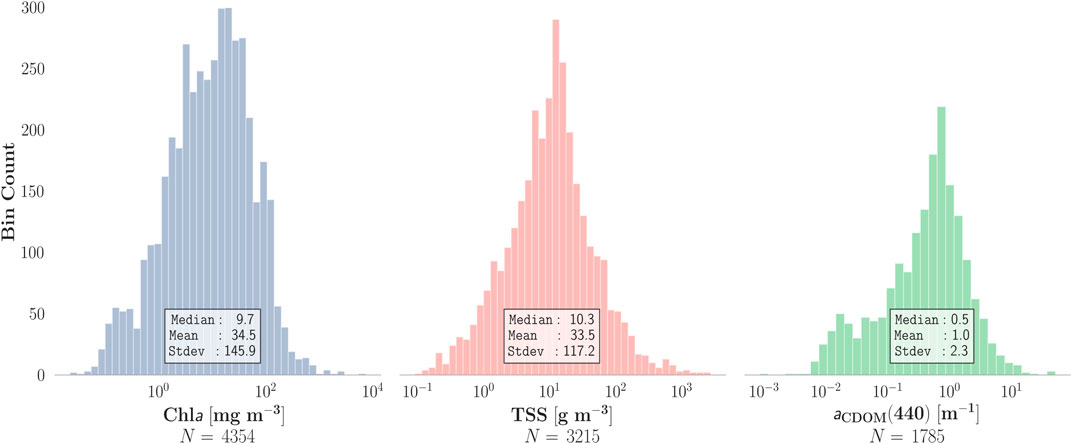
FIGURE 1. Distribution of Chla, TSS, and aCDOM (440) (data (Type A).
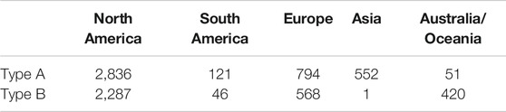
TABLE 1. Data distribution.
Type A data consists of radiometric and biogeochemical parameters that have been collected and assembled from various lakes, bays, estuaries, coast lines, and rivers from around the world (Figure 2), covering a wide range of trophic states and geographic locations (Pahlevan et al., 2020). The frequency distribution of Chla, Total Suspended Solids (TSS), and the absorption by CDOM at 443 nm (aCDOM (440)) is shown in Figure 1. Although our in situ measurements are not void of uncertainties, this dataset has proven useful for model development and validation (Pahlevan et al., 2020), representing the closest to ideal while still considering instrument and human errors.
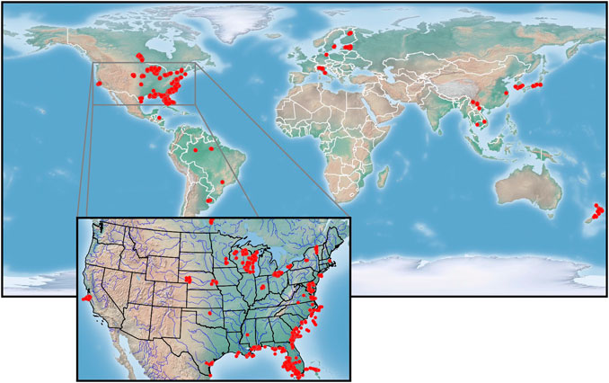
FIGURE 2. Geographic distribution of in situ measurements (Type A) (N = 4,354) Background map was obtained from http://www.shadedrelief.com/.
The radiometric quantity primarily used for model developments in this study is the remote sensing reflectance
Rrs(sr−-1) is determined using the water-leaving radiance Lw and downwelling irradiance Ed in the air, just above the water surface. Hyperspectral Rrs spectra were resampled according to the OLI’s relative spectral response functions. Furthermore, the data was preprocessed before being used as input into any machine learning models, with Rrs data transformed according to a robust median-centering interquartile range (IQR) scaling process (fit to the training data); and the Chla values being log-scaled, and transformed to be within the interval (−1, 1). Type A data were used for training and validation of the first MDN model (MDNA; Section Mixture Density Network Model Types), and for performance assessment against that of other Chla algorithms (Section Performance Assessment).
The satellite matchup dataset (Type B) is composed of two sources: Level-1TP OLI scenes, and in situ Chla measurements made during cruises, at buoys, or via site visits carried out through routine monitoring activities. The in situ data were obtained via a search of national/international water quality databases, such as the Water Quality Portal (WQP), NOAA’s Chesapeake Bay Interpretive Buoy System (CB), Environment and Climate Change Canada (ECCC), the World Ocean Database (WOD), and others. The data acquired from CB are near-surface calibrated fluorometry data, while remaining data represent near-surface or depth-integrated Chla determined via laboratory analyses. The application of Type B data is twofold: 1) to evaluate the performance of the MDN model applied to atmospherically corrected products
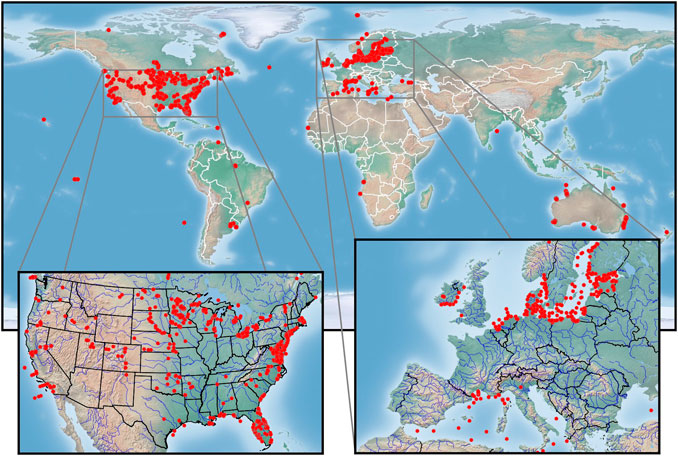
FIGURE 3. Geographic distribution of satellite matchups (Type B) (N = 3,371) Background map was obtained from http://www.shadedrelief.com/.
Radiative transfer theory details a series of equations that are concerned with the forward problem: given a set of parameters which describe the inherent optical properties (IOPs) of the water, concentrations of water constituents (e.g., Chla), and a set of boundary conditions, which limit the environment itself, how the relevant apparent optical properties (AOPs) can be discerned (Mobley, 1994). In the same manner, the standard target of a model in machine learning takes the form of a forward problem: given a set of independent variables, the goal is to find a function which approximates the relationship between these and the dependent variables. In particular, the relationship must be right-unique, which guarantees there is a single set of true outputs (y) for any given set of input (x) variables in a dataset D:
Plainly, for any input-output pair in a dataset, any samples with the same input must also maintain the same output (conditioned on noise). Inverse problems reverse the relationship however, i.e. switching x and y, which leads to violations of this core assumption. In natural environments, bio-optically active constituents and illumination conditions cause observed Rrs; the same set of input parameters, with perfect knowledge, should always lead to the same Rrs. In the inverse formulation, we attempt to instead determine bio-optical parameters and biogeochemical properties from the Rrs observations, and thus have the possibility of a single Rrs spectrum leading to multiple sets of valid parametric solutions (and so, multiple valid environments in which the spectrum might have been observed) (Pahlevan et al., 2020; Pahlevan et al., 2021).
Mixture Density Networks (MDN) (Bishop 1994) are a class of neural networks which attempt to address this one-to-many mapping (Sydor et al., 2004; Defoin-Platel and Chami 2007). Where a standard neural network (e.g. MLP) directly models the Rrs => Chla relationship, MDNs model a conditional probability distribution, i.e.,
with c mixture components and dimensionality d,
There are several viable AC methods suitable for OLI data processing; nonetheless we focused only on one processing chain, i.e., the SeaWiFS Data Analysis System (SeaDAS), the heritage ocean color AC processing scheme adopted for OLI (Franz et al., 2015). This processing approach is also adopted by the USGS Earth Resource Operation and Science center (EROS) to produce aquatic reflectance products, which are equivalent to Rrs products normalized by π. In this study, OLI images were not only fully processed to Rrs but also partially processed to output intermediate ρs that is corrected for atmospheric gaseous absorption, molecular scattering effects, and air-water interface multiple scattering phenomena (Gordon 1997). To compare the effects of AC schemes on Chla retrievals, a single OLI image was processed by three other methods: Polynomial based algorithm applied to MERIS (POLYMER) (Steinmetz et al., 2011), Atmospheric Correction for OLI lite (ACOLITE) (Vanhellemont and Ruddick 2018), and Case-2 Extreme Waters (C2X) (Brockmann et al., 2016) (Section Impacts of Atmospheric Correction).
To create satellite matchup datasets (Type B), SeaDAS-processed OLI scenes were paired with in situ measurements on same-day overpasses and the matchup criteria proposed in Bailey and Werdell (2006) was followed using strict spatiotemporal filters to remove matchups with questionable quality. A 3 × 3-element box centered on the closest geographic coordinates of the in situ measurement was used to select potential satellite observations (Figure 3), and any matchup was discarded if four or more pixels were flagged as invalid. Further, any cruise samples <500 m apart were considered duplicates and removed. Temporal mismatch criteria were further tightened for dynamic aquatic ecosystems (e.g., Chesapeake Bay, riverine systems) to 30 min to minimize the associated uncertainties. The median value of valid pixels within the 3 × 3-element box was then derived for each parameter and preprocessed in the same manner as the Type A data. All relevant reflectance products, including top-of-atmosphere reflectance
The naming convention used for MDN model developments follows the format listed in Table 2. Each of the MDN models was trained with 50% of the total available samples within the respective dataset, chosen uniformly at random (with the same set of samples used to train all ML models; Section Benchmarking). The remaining, held-out portion of the dataset was then used to test the models. The “bagging” scheme was also applied to all ML models—in order to ensure a fair comparison between algorithms—with 75% of the training data used per bagging estimator (without replacement), and an ensemble size of 10 estimators. All hyperparameters of the benchmark models were chosen via a 5-fold cross validation grid search on the training data. For a detailed discussion on MDN hyperparameters, see Supplementary Appendix C.
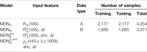
TABLE 2. MDN model types. VIS indicates OLI’s visible bands.
In those MDN models which utilize ancillary data, these features are added alongside their respective
In order to help prevent the models from learning spurious relationships due to temporal misalignment, we added one additional feature to all MDNB models, which represents the number of minutes between the satellite overpass and the in situ measurement, i.e.,
Given their previous application in the aquatic remote sensing area, MLP, SVM, and XGB were the main ML models identically trained and tested with the MDNA model. Due to its simple implementation and successful application in classification problems, K Nearest Neighbor (KNN) was also added as another benchmark (Altman 1992). In spite of its expected performance loss in waterbodies rich in organic or inorganic material, the OC3 model was also used as another benchmark (Franz et al., 2015). The MDNB models were further benchmarked against another XGB model, hereafter referred to by its name in original publication (BST), developed and tested by Cao et al. (2020).
To quantify performance, we primarily examined three metrics: Median Symmetric Accuracy (Morley et al., 2018), referred to as “Error” in all plots and tables; Symmetric Signed Percentage Bias (Morley et al., 2018), referred to as “Bias” in all plots and tables; and the slope of the least-squares linear regression line on the log-transformed data (Campbell 1995). All three have straightforward interpretations, though to clarify the first two:
• Median Symmetric Accuracy (“Error”) can be interpreted as a symmetric percentage error, equally penalizing over- and under-estimation. Lower values indicate better performance, with perfect accuracy being assigned a value of 0%.
• Symmetric Signed Percentage Bias (“Bias”), as with the former metric, is interpretable as a percentage bias that maintains symmetry between over- and under-estimation. Values closer to zero indicate better performance, with positive values indicating over-estimation and negative indicating under-estimation.
In the equations above (5–7), Chla denotes the in situ value and
The performance of
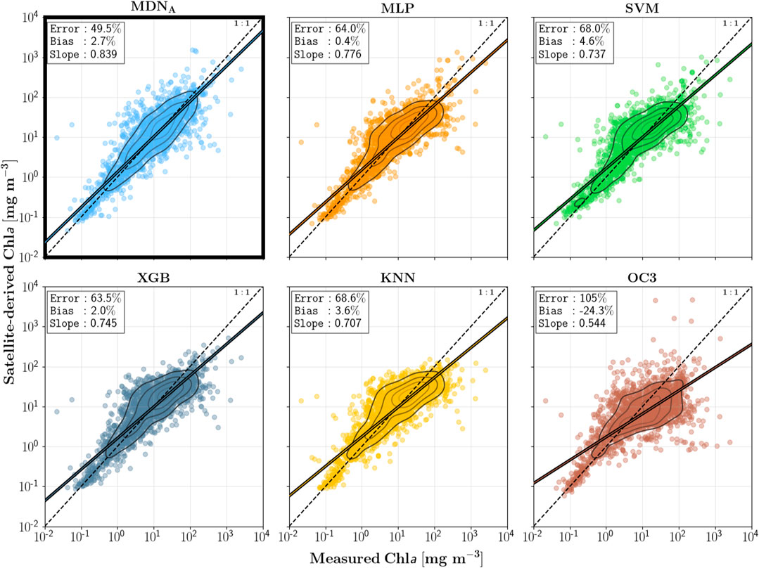
FIGURE 4. Performance of all algorithms on the in situ dataset (Type A; N = 2,177). MDNA, despite using suboptimal hyperparameters, still outperforms all other surveyed algorithms. The contour lines correspond with density estimates.
To gauge the level of noise introduced through the AC (SeaDAS), we also produced Chla scatter plots via
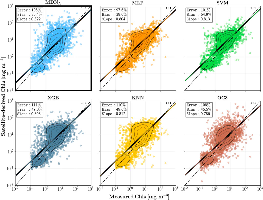
FIGURE 5. OLI-retrieved Chla evaluated using satellite matchups, i.e., Type B dataset (N = 3,371). SeaDAS was used for the atmospheric correction in all cases.
In spite of these issues, Landsat-matchup trained MDN model MDNB is to some extent capable of improving the accuracy as compared to that of the original (MDNA) model (Figure 6). In essence, the model accounts for some uncertainties inherent to the
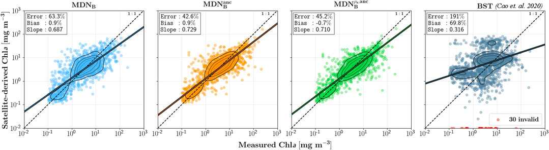
FIGURE 6. Performance assessment of MDNB models using half of the Type B dataset (N = 1,685). The performance of the original model by Cao et al. (2020) is included. Red dots indicate negative estimates or failure.
The different models examined in Section Methods are retrained using the full datasets, rather than splitting into training and/or testing sets. This allows for the model development to have the widest range of data available. Using the retrained models, two scenarios are demonstrated here.
As a first example, a natural color image of Lake Erie and the derived products during a harmful algal bloom event on Sept. 14th, 2015 was used (Figure 7). The black “x” markers indicate the positions of the three monitoring stations visited by the Great Lakes Environmental Research Laboratory (GLERL) within ±1 hr of Landsat-8 overpass. High concentrations of Chla in the southwestern section of the lake are evident in the natural color image generated from ρs products. The elevated backscatter evident in the natural color image of the northern and central Lake St. Claire discharging into Lake Erie is commonly attributed to suspended sediments and resuspension events (Bukata et al., 1988; Hawley and Lesht 1992; Czuba et al., 2011; Avouris and Ortiz, 2019). Table 3 contains the extracted Chla measurements and the Chla estimates from the MDN models. Although there is a slight temporal mismatch between Landsat-8 overpass and in situ measurements, there is a clear pattern in the results which quantitatively supports the accuracy improvement made by the MDN models.
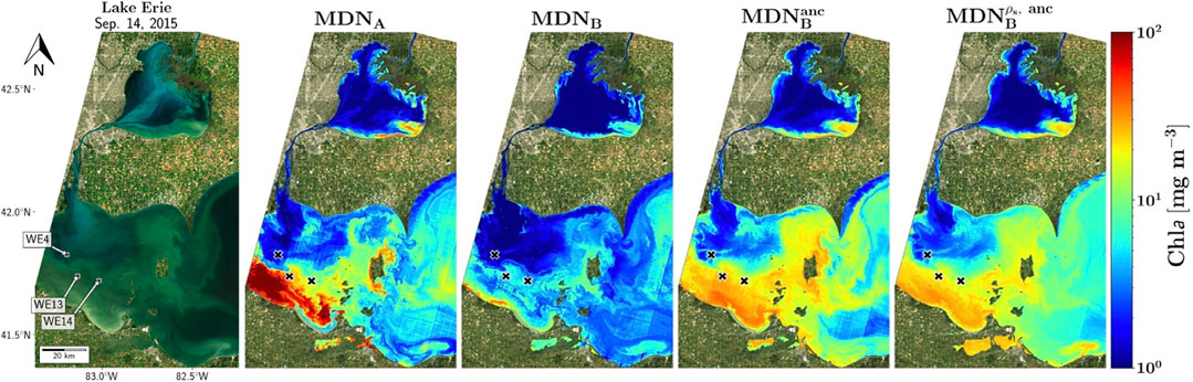
FIGURE 7. Algorithm estimates for Lake Erie (Sept. 14th, 2015), with a bloom event occurring in the south-western portion of the lake apparent in the natural color image (left column).
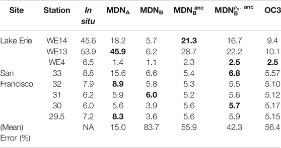
TABLE 3. In situ Chla data collected near-coincident (±1 h) with Landsat-8 overpasses. The estimated Chla from various MDN models and OC3 are also tabulated. See Figures 7 and 8 for the locations. Best performer for each station is boldfaced.
One point to note is the apparent underestimation of the MDN Type B models. This can be at least partially attributed to the AC frequently failing in highly eutrophic waters (Wang et al., 2019): since the MDNB models are only trained on samples (Figure 3 and Supplementary Appendix A) for which SeaDAS gives a valid result, there will necessarily be a bias toward lower concentration samples within the training data. This bias does not appear to be present in the MDNA model, as it would not have such a selection bias in its training set. Taking WE13 station as an example, we note that in spite of the reported concentrations >50 mg m−3, OC3 estimates a maximum of around 10.1 mg m−3, with the majority of examined areas below 11 mg m−3 (Table 3). MDNB exhibits similar behavior, possibly due to the previously discussed selection bias in the training data. However, when ancillary features are added to the model inputs (as is the case with
Our second example is comprised of a scene over the San Francisco Bay (SFB), imaged on April 27th, 2017 at 18:43 GMT (Figure 8), for which there were a few near-simultaneous in situ Chla measurements (Table 3) provided by SFB monthly cruises. In contrast to MDNB-derived maps, the map obtained from MDNA shows highly eutrophic areas (>20 mg·m−3) in the south bay region. Retrievals from MDNA were similar to in situ measurements (in the lower bay) except for the estimate at station 33—which is far greater than the measured concentrations (Table 3). This might be caused by any number of factors, not least of which being those biases inherent to the AC process. An interesting feature in Figure 8 is the Chla field outside the bay in the Pacific coasts (or in San Pablo Bay) that has been merely predicted by
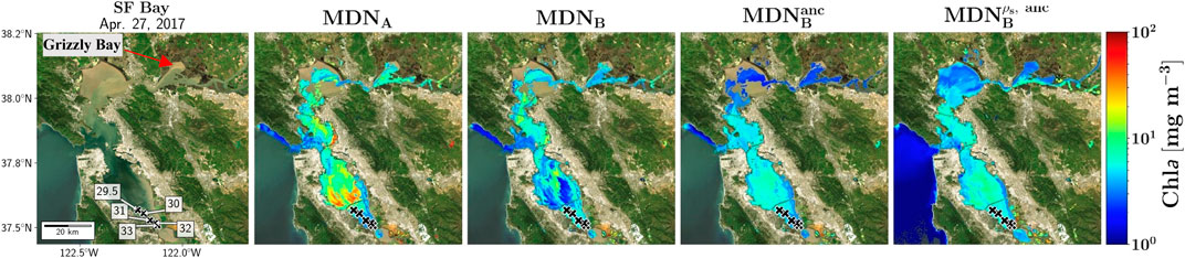
FIGURE 8. Algorithm estimates for San Francisco (SF) Bay (April 27 th, 2017) shown along the natural color image (left column). Note the successful retrievals via
The Time-series of estimated Chla are compared with in situ measurements in Figure 9. In this case, the in situ data (N ∼ 30) were measured via calibrated autonomous fluorometers deployed near-surface in Grizzly Bay, the northern section of the SFB region (Figure 8). The errors (Eq. 5) for the different models amounted to 54%, 41%, 120%, and 241% for
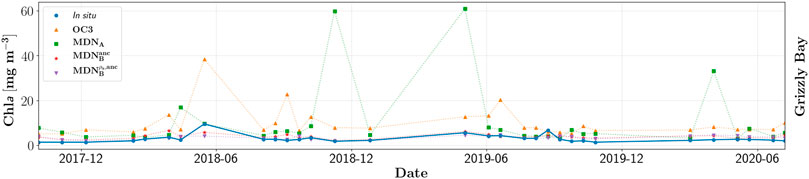
FIGURE 9. Time-series data extracted from in situ fluorometric Chla measurements along with estimates derived from different versions of MDN models and OC3.
Based on these results, one infers that the MDN is a promising model in retrieving Chla from OLI, offering improvements in accuracy over other current models. Here, we further address why this model is a likely choice for retrievals and demonstrate its strength in suppressing noise in Rrs compared to other ML models. This is followed by a discussion on the impacts of varying AC methods on the performance of MDNA and the implications of this research for studying and monitoring global waterbodies using Landsat-8 and other missions.
Neural network models have long been regarded as black-box models, with their complexity being a double-edge: providing more accurate solutions than have been previously available, at the cost of understanding the rationale in their estimations. This loss of explicability is of great concern for those involved in critical applications, due to the costs incurred in the event of failures. Without a source to identify as the cause—as is often the case in these models—the trust placed in the application is eroded. Recent research has led to a number of methods which allow for better model transparency, however. For instance, with many models it can be helpful to visualize the effect a given input feature has on the output of the model; in this case the effect of a certain band on the Chla estimation.
One such method to do this is called an Accumulated Local Effects (ALE) plot (Apley and Zhu 2016). The interested reader may also examine the literature for the related Partial Dependence (PD) plot—though these have the disadvantage of assuming independence between input features, and so are not the best choice in this case. ALE plots, on the other hand, calculate the effect of a feature conditional upon the other input features. Another way to explain this is, they examine the average change in prediction over a window around an input feature’s values, only conditioning upon other features in areas for which values exist in the data set. Figure 10 shows the ALE plots for the OLI bands, generated via the Type A data set. Note that the y-axis values correspond to the accumulated local effect, which can be thought of as “change in estimated Chla.” These plots indicate that 561 nm, when observed with a large magnitude, has the greatest (positive) effect on chlorophyll-a estimation. Not surprisingly, 482 nm also appears to significantly impact chlorophyll estimates with an inverse relationship: low magnitude reflectances indicating a higher than average chlorophyll-a value, and high magnitude reflectances indicating a lower than average chlorophyll-s value. On the other hand, since the 655-nm band does not fully cover Chla absorption at 676 nm, it appears to contain limited spectral information pertaining to Chla (see Helder et al. (2018)).
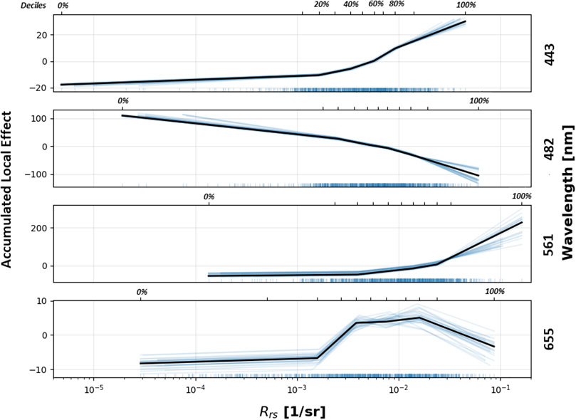
FIGURE 10. ALE plots showing the sensitivity of MDN Chla estimates, with respect to changes in the input spectral bands. Y-axes measure the accumulated local effect, which can be thought of as “change in estimated Chla.”
Although the primary processing scheme used here was SeaDAS, here, we underscore the importance and challenges associated with the AC. To that end, C2X, ACOLITE, and POLYMER, in addition to SeaDAS, were implemented to a sample OLI scene over Lake Peipsi, June 14th, 2016, followed by applying the MDNA model to all the derived Rrs products. Figure 11 shows the corresponding Chla map products. The inconsistency in the relative distribution and the overall magnitude of products is largely noticeable. For example, C2X appears to predict a large bloom in the center of the lake whereas other schemes provide values closer to the lake-wide average estimate. Moreover, SeaDAS and ACOLITE tend to estimate relatively high Chla in the southern and eastern basins while POLYMER retrieves only slightly higher-than-average estimates. Same-day in situ Chla measurements and the estimated Chla from MDNA and OC3 from the four processors are included in Table 4 (Alikas et al., 2015). Despite that the in situ dataset does not represent the entirety of the ecosystem, it allows to better comprehend the complexity induced through the AC process and how confusing the output products may be. Given the statistics in Table 4, there is no single processor that distinctly outperforms the rest for this instance of OLI image and/or lake. It is worth noting that while SeaDAS, ACOLITE, and POLYMER statistically yield better Chla estimates via MDNA, retrieved Chla values from C2X through OC3 resembles in situ samples more closely. This observation and the discrepancies in the performances further corroborates the need for an improved AC method for the OLI data processing to achieve the theoretical limit shown in Figure 4.
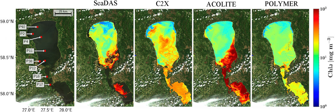
FIGURE 11. An OLI scene acquired on June 14th, 2016 processed via four different atmospheric correction methods. The MDNA model was used to generate Chla from the output of the processors.
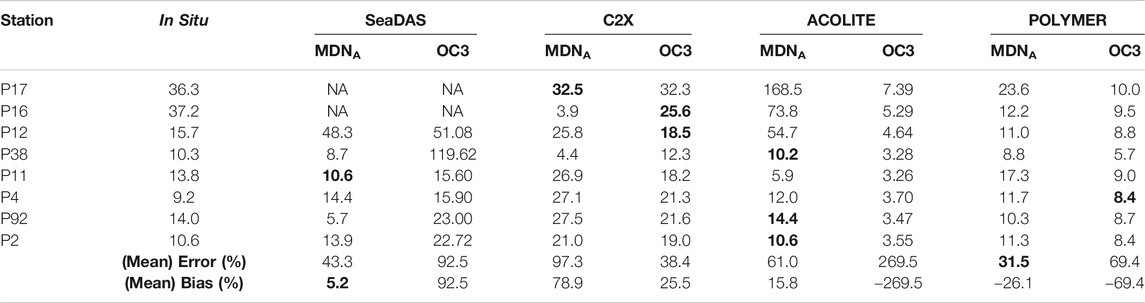
TABLE 4. In situ Chla and retrieved Chla derived from four different AC processors by applying MDNA and OC3. The boldfaced values correspond to best estimates at each station.
Landsat-8 data, when combined with the data from Sentinel-2 and -3, are expected to allow for near-daily global observations of inland and coastal waters. Irrespective of differences in their observation modalities, creating consistent Chla products is key for successful assessment and monitoring of these ecosystems. Considering the missing RE measurements in the OLI suite of observations however, retrieving Chla as accurately as that with MSI and OLCI appears challenging. Although the number of matchups assessed is different, comparing to our previous results (Pahlevan et al., 2020), it can be inferred that Rrs, or their equivalent
In addition to SeaDAS, we also implemented and tested ACOLITE and POLYMER to assess the performance of MDNA models. Our analyses showed that these alternative models yield Chla as inaccurate as that from SeaDAS (Figure 5). The performance of MDNB and MDNBanc using
Spatial and temporal mismatches inherent to satellite matchups introduce further uncertainties in our assessments. Of concern is, in particular, our same-day criteria. We made an attempt to diminish the impact of this noise source by supplying
The inclusion of ancillary data, such as the solar angles, sensor viewing angle, wind data, water vapor, and others, enhanced the model performance noticeably when added to model input features, regardless of AC processor. The improvements stem from how SeaDAS utilizes the ancillary information itself (Mobley et al., 2016) while some of the parameters are not often used, e.g., wind speed, wind angle. In some cases, the algorithm may apply simplifications, for example to reduce computational burden, that may preclude a rigorous integration of ancillary data in the process. In particular, we found that our model is very sensitive to sensor azimuth angles, which change sign for the two adjacent focal plane modules (Markham et al., 2014). Our spatial analysis suggested that including these angles yield alternate low-high Chla for the odd and even focal plane modules (Pahlevan et al., 2017b); hence, we decided to discard this information, which led to more spatially uniform maps. Further, it is worth pointing out that most ancillary variables (e.g., water vapor concentration) are coarse-resolution features with little to no per-pixel variability. Therefore, any fine structures or patterns seen in the estimates can only be influenced by the spectral information itself.
This work introduces a great number of potential directions for exploration. From the perspective of the aquatic remote sensing field as a whole, it is yet to be determined how the MDN model fares when applied to other missions. In the future, the performance evaluation is expected to be carried out for other ocean color missions, such as MODIS, which do not measure in the RE region but provide relevant spectral content in the vicinity of 750-nm region. Similarly, the MDN developed for OLI’s visible bands might be further extended by including the panchromatic band to further constrain the solution space (Castagna et al., 2020). As the atmospheric correction process has been shown to introduce significant errors in downstream products of such missions, and ρs being a feasible substitute to bypass portions of this process, the question becomes whether it is possible to bypass AC completely and allow for direct retrieval of the relevant biogeochemical properties. Alternatively: whether there are certain AC-specific parameters which might be tuned, in order to provide a more amenable input for learning the product inverse function.
Other directions include those focused more on ML, and the MDN itself. For instance, the MDN model also has the capability to simultaneously estimate multiple products; to what extent do the inclusion of additional variables in the model output (e.g., TSS) affect performance? Intuitively these additions should serve only to improve accuracy overall, given the additional information of target covariances—but which products might be estimated synergistically is yet to be explored.
More theoretically, we might ask if there are non-Gaussian distributions (e.g., Laplace, which may better represent the data); or, whether the learned mixture components might relate to the physical environments of the samples assigned. Further exploration is required in regard to the model hyperparameters, and the mixture components especially. There are very likely advancements in the field of machine learning (e.g., activation functions, batch normalization procedures, convolutional/temporal architectures, etc.) which could also be applied to enhance retrievals—though potentially requiring alternative data formulations, such as incorporating spatial or temporal information.
In this work, we have gathered a global dataset of both Rrs – Chla and
The MDN algorithm represents a promising step toward the goal of global simultaneous biophysical and biogeochemical variable retrieval, in the context of aquatic remote sensing. While results are promising, much work is left to be done in both data acquisition and model validation. To truly design a global-scale model, capable of approximating an inverse solution to the radiative transfer equations, significantly more data is required. Simultaneously retrieving all parameters of interest to the community requires the potential dataset to have the necessary information to learn relevant covariances in all atmospheric conditions. Just as important, the various sources of uncertainty and misalignment must also be minimized in order for the model to accurately learn these relationships.
We conclude with broad discussions of other justifications and benefits, analyses on the hyperparameters, implications of the model within the broader community, and potential directions for further experimentation. These discussions are far from exhaustive, but we hope they will provide the seed for future advancements in remote sensing.
The datasets presented in this article are not readily available because data ownership belongs to partner organizations. The data will be published in the future upon agreement with data providers. Requests to access the datasets should be directed to TmltYS5wYWhsZXZhbkBuYXNhLmdvdi4= All the developed codes are available through https://github.com/STREAM-RS/STREAM-RS.
NP: Conceptualization; BS, JS, RM, CG, MB, CB, SR, RE, and VF: Data curation; BS: Formal analysis; NP: Funding acquisition; NP and BS: Investigation; BS: Methodology; NP: Project administration; NP: Resources; BS: Software; NP: Supervision; BS: Validation; BS: Visualization; NP and BS: Roles/Writing – original draft; NP: Writing – review and editing.
We acknowledge the European Union’s Horizon 2020 research and innovation program (grant agreement No. 730066, EOMORES) to support in situ data collection in Estonian inland waters. Nima Pahlevan is funded under NASA ROSES contract # 80HQTR19C0015, Remote Sensing of Water Quality element, and the USGS Landsat Science Team Award # 140G0118C0011.
Authors BS and NP were employed by the company Science Systems and Applications Inc.
The remaining authors declare that the research was conducted in the absence of any commercial or financial relationships that could be construed as a potential conflict of interest.
We would like to recognize all the individuals and entities that acquired, processed, and prepared in situ data that are central to the development of global algorithms. The principal investigators providing the data include Caren Binding, Daniela Gurlin, Steve Greb, Bunkei Matsushita, Anatoly Gitelson, Wesley Moses, Moritz Lehman, and Michael Ondrusek. We also acknowledge NASA’s support in creating and maintaining SeaBASS.
The Supplementary Material for this article can be found online at: https://www.frontiersin.org/articles/10.3389/frsen.2020.623678/full#supplementary-material.
1Comparison with Pahlevan et al. (2020) is possible through the relationship: Error = 100 x (MAE-1).
Alikas, K., Kangro, K., Randoja, R., Philipson, P., Asuküll, E., Pisek, J., et al. (2015). Satellite-based products for monitoring optically complex inland waters in support of EU water framework directive. Int. J. Rem. Sens. 36, 4446–4468. doi:10.1080/01431161.2015.1083630
Allan, M. G., Hamilton, D. P., Hicks, B., and Brabyn, L. (2015). Empirical and semi-analytical chlorophyll a algorithms for multi-temporal monitoring of New Zealand lakes using Landsat. Environ. Monit. Assess. 187, 364. doi:10.1007/s10661-015-4585-4
Altman, N. S. (1992). An introduction to kernel and nearest-neighbor nonparametric regression. Am. Statistician 46, 175–185. doi:10.2307/2685209
Apley, D. W., and Zhu, J. (2016). Visualizing the effects of predictor variables in black box supervised learning models. J. Royal Stat. Soc. Series B (Stat. Met.). 82 (4), 12377. doi:10.1111/rssb.12377 arXiv preprint arXiv:1612.08468.
Avouris, D. M., and Ortiz, J. D. (2019). Validation of 2015 Lake Erie MODIS image spectral decomposition using visible derivative spectroscopy and field campaign data. J. Great Lake. Res. 45, 466–479. doi:10.1016/j.jglr.2019.02.005
Bailey, S. W., Franz, B. A., and Werdell, P. J. (2010). Estimation of near-infrared water-leaving reflectance for satellite ocean color data processing. Opt. Exp. 18, 7521–7527. doi:10.1364/OE.18.007521
Bailey, S. W., and Werdell, P. J. (2006). A multi-sensor approach for the on-orbit validation of ocean color satellite data products. Rem. Sens. Environ. 102, 12–23. doi:10.1016/j.rse.2006.01.015
Bishop, C. M. (1994). Mixture density networks NCRG/94/004. Birmingham, United Kingdom: Aston UniversityAvailable at: http://www.ncrg.aston.ac.uk.
Bresciani, M., Cazzaniga, I., Austoni, M., Sforzi, T., Buzzi, F., Morabito, G., et al. (2018). Mapping phytoplankton blooms in deep subalpine lakes from Sentinel-2A and Landsat-8. Hydrobiologia 824, 197–214. doi:10.1007/s10750-017-3462-2
Brockmann, C., Doerffer, R., Peters, M., Kerstin, S., Embacher, S., and Ruescas, A. (2016). Evolution of the C2RCC neural network for Sentinel 2 and 3 for the retrieval of ocean colour products in normal and extreme optically complex waters. ESA-SP 740, 54.
Bukata, R., Jerome, J., Bruton, J., Jain, S., and Zwick, H. (1981). Optical water quality model of Lake Ontario. 1: determination of the optical cross sections of organic and inorganic particulates in Lake Ontario. Appl. Optic. 20, 1696–1703. doi:10.1364/AO.20.001696
Bukata, R. P., Jerome, J. H., and Bruton, J. E. (1988). Particulate concentrations in Lake St. Clair as recorded by a shipborne multispectral optical monitoring system. Rem. Sens. Environ. 25, 201–229. doi:10.1016/0034-4257(88)90101-0
Bukata, R. P., Jerome, J. H., Kondratyev, K. Y., and Pozdnyakox, D. V. (1995). Optical properties and remote sensing of inland and coastal waters. New York, NY: CRC Press.
Campbell, J. W. (1995). The lognormal distribution as a model for bio-optical variability in the sea. J. Geophys. Res. 100, 13237–13254. doi:10.1029/95jc00458
Cao, Z., Ma, R., Duan, H., Pahlevan, N., Melack, J., Shen, M., et al. (2020). A machine learning approach to estimate chlorophyll-a from Landsat-8 measurements in inland lakes. Rem. Sens. Environ. 248, 111974. doi:10.1016/j.rse.2020.111974
Castagna, A., Simis, S., Dierssen, H., Vanhellemont, Q., Sabbe, K., and Vyverman, W. (2020). Extending Landsat 8: retrieval of an orange contra-band for inland water quality applications. Rem. Sens. 12, 637. doi:10.3390/rs12040637
Chang, C.-C., and Lin, C.-J. (2011). LIBSVM: a library for support vector machines. ACM Trans. Intell. Syst. Technol. 2, 1–27. doi:10.1145/1961189.1961199
Chen, J., Cui, T., Ishizaka, J., and Lin, C. (2014). A neural network model for remote sensing of diffuse attenuation coefficient in global oceanic and coastal waters: exemplifying the applicability of the model to the coastal regions in eastern China seas. Rem. Sens. Environ. 148, 168–177. doi:10.1016/j.rse.2014.02.019
Chen, T., and Guestrin, C. (2016). “Xgboost: a scalable tree boosting system,” in Proceedings of the 22nd acm sigkdd international conference on knowledge discovery and data mining, San Francisco, CA, August 13–17, 2016, 785–794.
Clarke, G. L., Ewing, G. C., and Lorenzen, C. J. (1970). Spectra of backscattered light from the sea obtained from aircraft as a measure of chlorophyll concentration. Science 167, 1119–1121. doi:10.1126/science.167.3921.1119
Concha, J. A., and Schott, J. R. (2016). Retrieval of color producing agents in case 2 waters using Landsat 8. Rem. Sens. Environ. 185, 95–107. doi:10.1016/j.rse.2016.03.018
Czuba, J. A., Best, J. L., Oberg, K. A., Parsons, D. R., Jackson, P. R., Garcia, M. H., et al. (2011). Bed morphology, flow structure, and sediment transport at the outlet of Lake Huron and in the upper St. Clair River. J. Great Lake. Res. 37, 480–493. doi:10.1016/j.jglr.2011.05.011
Defoin-Platel, M., and Chami, M. (2007). How ambiguous is the inverse problem of ocean color in coastal waters? J. Geophys. Res.: Oceans 112, C003847. doi:10.1029/2006JC003847
Doerffer, R., and Schiller, H. (2007). The MERIS case 2 water algorithm. Int. J. Rem. Sens. 28, 517–535. doi:10.1080/01431160600821127
Esaias, W. E., Abbott, M. R., Barton, I., Brown, O. B., Campbell, J. W., Carder, K. L., et al. (1998). An overview of MODIS capabilities for ocean science observations. IEEE Trans. Geosci. Rem. Sens. 36, 1250–1265. doi:10.1109/36.701076
Franz, B. A., Bailey, S. W., Kuring, N., and Werdell, P. J. (2015). ocean Color measurements with the operational land imager on landsat-8: implementation and evaluation in SeaDAS. J. Appl. Remote Sens. 9, 096070. doi:10.1117/1.jrs.9.096070
Freitas, F. H., and Dierssen, H. M. (2019). Evaluating the seasonal and decadal performance of red band difference algorithms for chlorophyll in an optically complex estuary with winter and summer blooms. Rem. Sens. Environ. 231, 111228. doi:10.1016/j.rse.2019.111228
Gilerson, A., Carrizo, C., Foster, R., and Harmel, T. (2018). Variability of the reflectance coefficient of skylight from the ocean surface and its implications to ocean color. Opt. Exp. 26, 9615–9633. doi:10.1364/OE.26.009615
Gitelson, A. A., Schalles, J. F., and Hladik, C. M. (2007). Remote chlorophyll-a retrieval in turbid, productive estuaries: Chesapeake Bay case study. Rem. Sens. Environ. 109, 464–472. doi:10.1016/j.rse.2007.01.016
Gitelson, A. (1992). The peak near 700 nm on radiance spectra of algae and water: relationships of its magnitude and position with chlorophyll concentration. Int. J. Rem. Sens. 13, 3367–3373. doi:10.1080/01431169208904125
Gordon, H. R., Clark, D. K., Brown, J. W., Brown, O. B., Evans, R. H., and Broenkow, W. W. (1983). Phytoplankton pigment concentrations in the Middle Atlantic Bight: comparison of ship determinations and CZCS estimates. Appl. Optic. 22, 20–36. doi:10.1364/ao.22.000020
Gordon, H. R., Clark, D. K., Mueller, J. L., and Hovis, W. A. (1980). Phytoplankton pigments from the nimbus-7 coastal zone color scanner: comparisons with surface measurements. Science 210, 63–66. doi:10.1126/science.210.4465.63
Gordon, H. R. (1997). Atmospheric correction of ocean color imagery in the Earth Observing System era. J. Geophys. Res. 102, 17081–17106. doi:10.1029/96jd02443
Goward, S. N., Williams, D. L., Arvidson, T., Rocchio, L. E., Irons, J. R., Russell, C. A., et al. (2017). Landsat’s enduring legacy: pioneering global Land observations from space. Photog. Engin. Remote Sens. 84 (1), 9–10. doi:10.14358/PERS.84.1.9
Gower, J., King, S., Borstad, G., and Brown, L. (2005). Detection of intense plankton blooms using the 709 nm band of the MERIS imaging spectrometer. Int. J. Rem. Sens. 26, 2005–2012. doi:10.1080/01431160500075857
Gower, J., Lin, S., and Borstad, G. (1984). The information content of different optical spectral ranges for remote chlorophyll estimation in coastal waters. Int. J. Rem. Sens. 5, 349–364. doi:10.1080/01431168408948813
Gross, L., Thiria, S., Frouin, R., and Mitchell, B. G. (2000). Artificial neural networks for modeling the transfer function between marine reflectance and phytoplankton pigment concentration. J. Geophys. Res. 105, 3483–3495. doi:10.1029/1999jc900278
Han, L., Rundquist, D., Liu, L., Fraser, R., and Schalles, J. (1994). The spectral responses of algal chlorophyll in water with varying levels of suspended sediment. Int. J. Rem. Sens. 15, 3707–3718. doi:10.1080/01431169408954353
Harding, L. W., Itsweire, E. C., and Esaias, W. E. (1994). Estimates of phytoplankton biomass in the Chesapeake Bay from aircraft remote sensing of chlorophyll concentrations, 1989-92. Rem. Sens. Environ. 49, 41–56. doi:10.1016/0034-4257(94)90058-2
Harmel, T., Chami, M., Tormos, T., Reynaud, N., and Danis, P.-A. (2018). Sunglint correction of the multi-spectral instrument (MSI)-SENTINEL-2 imagery over inland and sea waters from SWIR bands. Rem. Sens. Environ. 204, 308–321. doi:10.1016/j.rse.2017.10.022
Hawley, N., and Lesht, B. M. (1992). Sediment resuspension in lake St. Clair. Limnol. Oceanogr. 37, 1720–1737. doi:10.4319/lo.1992.37.8.1720
Helder, D., Markham, B., Morfitt, R., Storey, J., Barsi, J., Gascon, F., et al. (2018). Observations and recommendations for the calibration of Landsat 8 OLI and Sentinel 2 MSI for improved data interoperability. Rem. Sens. 10, 1340. doi:10.3390/rs10091340
Hieronymi, M., Müller, D., and Doerffer, R. (2017). The OLCI neural network swarm (ONNS): a bio-geo-optical algorithm for open ocean and coastal waters. Front. Marine Sci. 4, 140. doi:10.3389/fmars.2017.0014
Hinton, G. E. (1990). “Connectionist learning procedures,” in Machine learning. Amsterdam, Netherlands: Elsevier, 555–610.
Hyndman, R. J., and Koehler, A. B. (2006). Another look at measures of forecast accuracy. Int. J. Forecast. 22, 679–688. doi:10.1016/j.ijforecast.2006.03.001
Ilori, C. O., Pahlevan, N., and Knudby, A. (2019). Analyzing performances of different atmospheric correction techniques for Landsat 8: application for coastal remote sensing. Rem. Sens. 11, 469. doi:10.3390/rs11040469
Ioannou, I., Gilerson, A., Gross, B., Moshary, F., and Ahmed, S. (2011). Neural network approach to retrieve the inherent optical properties of the ocean from observations of MODIS. Appl. Optic. 50, 3168–3186. doi:10.1364/AO.50.003168
IOCCG (2000). “Remote sensing of ocean colour in coastal, and other optically-complex, waters,”in Reports of the International Ocean-Colour Coordinating Group. Editor S. Sathyendranath (Canada: IOCCG).
Irons, J. R., Dwyer, J. L., and Barsi, J. A. (2012). The next Landsat satellite: the Landsat data continuity mission. Rem. Sens. Environ. 122, 11–21. doi:10.1016/j.rse.2011.08.026
Jamet, C., Loisel, H., and Dessailly, D. (2012). Retrieval of the spectral diffuse attenuation coefficient Kd (λ) in open and coastal ocean waters using a neural network inversion. J. Geophys. Res.: Oceans 117 (C10), 8076. doi:10.1029/2012jc008076
Kajiyama, T., D’Alimonte, D., and Zibordi, G. (2018). Algorithms merging for the determination of chlorophyll-${a} $ concentration in the Black sea. Geosci. Rem. Sens. Lett. IEEE. 16, 677–681. doi:10.1109/LGRS.2018.2883539
Kay, S., Hedley, J. D., and Lavender, S. (2009). Sun glint correction of high and low spatial resolution images of aquatic scenes: a review of methods for visible and near infrared wavelengths. Rem. Sens. 1, 33. doi:10.3390/rs1040697
Khorram, S., Catts, G. P., Cloern, J. E., and Knight, A. W. (1987). Modeling of estuarne chlorophyll a from an airborne scanner. IEEE Trans. Geosci. Rem. Sens. 25, 662–669. doi:10.1109/tgrs.1987.289735
Kuhn, C., de Matos Valerio, A., Ward, N., Loken, L., Sawakuchi, H. O., Kampel, M., et al. (2019). Performance of Landsat-8 and Sentinel-2 surface reflectance products for river remote sensing retrievals of chlorophyll-a and turbidity. Rem. Sens. Environ. 224, 104–118. doi:10.1016/j.rse.2019.01.023
Kwiatkowska, E. J., and Fargion, G. S. (2003). Application of machine-learning techniques toward the creation of a consistent and calibrated global chlorophyll concentration baseline dataset using remotely sensed ocean color data. IEEE Trans. Geosci. Rem. Sens. 41, 2844–2860. doi:10.1109/tgrs.2003.818016
Le, C., Hu, C., English, D., Cannizzaro, J., Chen, Z., Feng, L., et al. (2013). Towards a long-term chlorophyll-a data record in a turbid estuary using MODIS observations. Prog. Oceanogr. 109, 90–103. doi:10.1016/j.pocean.2012.10.002
Makridakis, S. (1993). Accuracy measures: theoretical and practical concerns. Int. J. Forecast. 9, 527–529. doi:10.1016/0169-2070(93)90079-3
Manuel, A., Blanco, A., Tamondong, A., Jalbuena, R., Cabrera, O., and Gege, P. (2020). Optmization of bio-optical model parameters for turbid lake water quality estimation using Landsat 8 and wasi-2D. Int. Arch. Photogram. Rem. Sens. Spatial Inf. Sci. 11, 67–72. doi:10.5194/isprs-archives-xlii-3-w11-67-2020
Markham, B., Barsi, J., Kvaran, G., Ong, L., Kaita, E., Biggar, S., et al. (2014). Landsat-8 operational land imager radiometric calibration and stability. Rem. Sens. 6, 12275–12308. doi:10.3390/rs61212275
Markham, B. L., Barsi, J. A., Morfitt, R., Choate, M., Montanaro, M., Arvidson, T., et al. (2015). “Landsat 8: status and on-orbit performance,” in SPIE remote sensing. Bellingham, WA: International Society for Optics and Photonics, 963908.
Mittenzwey, K. H., Ullrich, S., Gitelson, A., and Kondratiev, K. (1992). Determination of chlorophyll a of inland waters on the basis of spectral reflectance. Limnol. Oceanogr. 37, 147–149. doi:10.4319/lo.1992.37.1.0147
Mobley, C. D. (1999). Estimation of the remote-sensing reflectance from above-surface measurements. Appl. Optic. 38, 7442–7455. doi:10.1364/ao.38.007442
Mobley, C. D. (1994). Light and Water: radiative transfer in natural waters. Cambridge, MA: Academic Press, Inc.
Mobley, C. D., Werdell, J., Franz, B., Ahmad, Z., and Bailey, S. (2016). Atmospheric correction for satellite ocean color radiometry. Front. Earth Sci. 2019, 145. doi:10.3389/feart.2019.00145 NASA/TM-2016-217551, GSFC-E-DAA-TN35509
Morley, S. K., Brito, T. V., and Welling, D. T. (2018). Measures of model performance based on the log accuracy ratio. Space Weather 16, 69–88. doi:10.1002/2017sw001669
Munday, J., and Zubkoff, P. L. (1981). Remote sensing of dinoflagellate blooms in a turbid estuary. Photogramm. Eng. Rem. Sens. 47, 523–531.
Neil, C., Spyrakos, E., Hunter, P. D., and Tyler, A. N. (2019). A global approach for chlorophyll-a retrieval across optically complex inland waters based on optical water types. Rem. Sens. Environ. 229, 159–178. doi:10.1016/j.rse.2019.04.027
O’Reilly, J. E., Maritorena, S., Mitchell, B. G., Siegel, D. A., Carder, K. L., Garver, S. A., et al. (1998). Ocean color chlorophyll algorithms for SeaWiFS. J. Geophys. Res. 103, 24937–24953. doi:10.1029/98jc02160
Pahlevan, N., Roger, J. C., and Ahmad, Z. (2017a). Revisiting short-wave-infrared (SWIR) bands for atmospheric correction in coastal waters. Optic Express 25, 6015–6035. doi:10.1364/OE.25.006015
Pahlevan, N., Schott, J. R., Franz, B. A., Zibordi, G., Markham, B., Bailey, S., et al. (2017b). Landsat 8 remote sensing reflectance (Rrs) products: evaluations, intercomparisons, and enhancements. Rem. Sens. Environ. 190, 289–301. doi:10.1016/j.rse.2016.12.030
Pahlevan, N., Lee, Z., Wei, J., Schaff, C., Schott, J., and Berk, A. (2014). On-orbit radiometric characterization of OLI (Landsat-8) for applications in aquatic remote sensing. Rem. Sens. Environ. 154, 272–284. doi:10.1016/j.rse.2014.08.001
Pahlevan, N., Smith, B., Binding, C., Gurlin, D., Li, L., Bresciani, M., et al. (2021). Hyperspectral retrievals of phytoplankton absorption and chlorophyll-a in inland and nearshore coastal waters. Rem. Sens. Envi. 253, 112200. doi:10.1016/j.rse.2020.112200
Pahlevan, N., Smith, B., Schalles, J., Binding, C., Cao, Z., Ma, R., et al. (2020). Seamless retrievals of chlorophyll-a from Sentinel-2 (MSI) and Sentinel-3 (OLCI) in inland and coastal waters: a machine-learning approach. Rem. Sens. Environ. 240, 111604. doi:10.1016/j.rse.2019.111604
Rundquist, D. C., Han, L., Schalles, J. F., and Peake, J. S. (1996). Remote measurement of algal chlorophyll in surface waters: the case for the first derivative of reflectance near 690 nm. Photogramm. Eng. Rem. Sens. 62, 195–200.
Ryu, J.-H., Han, H.-J., Cho, S., Park, Y.-J., and Ahn, Y.-H. (2012). Overview of geostationary ocean color imager (GOCI) and GOCI data processing system (GDPS). Ocean Sci. J. 47, 223–233. doi:10.1007/s12601-012-0024-4
Schiller, H., and Doerffer, R. (1999). Neural network for emulation of an inverse model operational derivation of Case II water properties from MERIS data. Int. J. Rem. Sens. 20, 1735–1746. doi:10.1080/014311699212443
Seegers, B. N., Stumpf, R. P., Schaeffer, B. A., Loftin, K. A., and Werdell, P. J. (2018). Performance metrics for the assessment of satellite data products: an ocean color case study. Optic Express 26, 7404–7422. doi:10.1364/OE.26.007404
Smith, R. C., and Baker, K. S. (1982). Oceanic chlorophyll concentrations as determined by satellite (Nimbus-7 coastal zone color scanner). Mar. Biol. 66, 269–279. doi:10.1007/bf00397032
Snyder, J., Boss, E., Weatherbee, R., Thomas, A. C., Brady, D., and Newell, C. (2017). Oyster aquaculture site selection using Landsat 8-derived sea surface temperature, turbidity, and chlorophyll a. Front. Marine Sci. 4, 190. doi:10.3389/fmars.2017.00190
Spyrakos, E., O’Donnell, R., Hunter, P. D., Miller, C., Scott, M., Simis, S. G., et al. (2018). Optical types of inland and coastal waters. Limnol. Oceanogr. 63, 846–870. doi:10.1002/lno.10674
Steinmetz, F., Deschamps, P. Y., and Ramon, D. (2011). Atmospheric correction in presence of sun glint: application to MERIS. Optic Express 19, 9783–9800. doi:10.1364/oe.19.009783
Sydor, M., Gould, R. W., Arnone, R. A., Haltrin, V. I., and Goode, W. (2004). Uniqueness in remote sensing of the inherent optical properties of ocean water. Appl. Optic. 43, 2156–2162. doi:10.1364/ao.43.002156
Tofallis, C. (2015). A better measure of relative prediction accuracy for model selection and model estimation. J. Oper. Res. Soc. 66, 1352–1362. doi:10.1057/jors.2014.103
Trinh, R. C., Fichot, C. G., Gierach, M. M., Holt, B., Malakar, N. K., Hulley, G., et al. (2017). Application of Landsat 8 for monitoring impacts of wastewater discharge on coastal water quality. Front. Marine Sci. 4, 329. doi:10.3389/fmars.2017.00329
Vanhellemont, Q., and Ruddick, K. (2018). Atmospheric correction of metre-scale optical satellite data for inland and coastal water applications. Rem. Sens. Environ. 216, 586–597. doi:10.1016/j.rse.2018.07.015
Vilas, L. G., Spyrakos, E., and Palenzuela, J. M. T. (2011). Neural network estimation of chlorophyll a from MERIS full resolution data for the coastal waters of Galician rias (NW Spain). Rem. Sens. Environ. 115, 524–535. doi:10.1016/j.rse.2010.09.021
Vos, W., Donze, M., and Buiteveld, H. (1986). On the reflectance spectrum of algae in water: the nature of the peak at 700 nm and its shift with varying algal concentration. Delft, Netherlands: Delft University of Technology, Faculty of Civil Engineering.
Wang, D., Ma, R., Xue, K., and Loiselle, S. (2019). The assessment of Landsat-8 OLI atmospheric correction algorithms for inland waters. Rem. Sens. 11, 169. doi:10.3390/rs11020169
Wang, M., and Bailey, S. W. (2001). Correction of sun glint contamination on the SeaWiFS ocean and atmosphere products. Appl. Optic. 40, 4790–4798. doi:10.1364/ao.40.004790
Wang, M., Liu, X., Jiang, L., Son, S., Sun, J., Shi, W., et al. (2014). “Evaluation of VIIRS ocean color products,” in Ocean remote sensing and monitoring from SpaceInternational society for optics and photonics, 92610E.
Warren, M. A., Simis, S. G., Martinez-Vicente, V., Poser, K., Bresciani, M., Alikas, K., et al. (2019). Assessment of atmospheric correction algorithms for the Sentinel-2A multispectral imager over coastal and inland waters. Rem. Sens. Environ. 225, 267–289. doi:10.1016/j.rse.2019.03.018
Watanabe, F. S., Alcântara, E., Rodrigues, T. W., Imai, N. N., Barbosa, C. C., and Rotta, L. H. (2015). Estimation of chlorophyll-a concentration and the trophic state of the Barra Bonita hydroelectric reservoir using OLI/Landsat-8 images. Int. J. Environ. Res. Publ. Health 12, 10391–10417. doi:10.3390/ijerph120910391
Werdell, P. J., Bailey, S. W., Franz, B. A., Harding, L. W., Feldman, G. C., and McClain, C. R. (2009). Regional and seasonal variability of chlorophyll-a in Chesapeake Bay as observed by SeaWiFS and MODIS-Aqua. Rem. Sens. Environ. 113, 1319–1330. doi:10.1016/j.rse.2009.02.012
Wezernak, C., Tanis, F., and Bajza, C. (1976). Trophic state analysis of inland lakes. Rem. Sens. Environ. 5, 147–164. doi:10.1016/0034-4257(76)90045-6
Wynne, T., Stumpf, R., and Briggs, T. (2013). Comparing MODIS and MERIS spectral shapes for cyanobacterial bloom detection. Int. J. Rem. Sens. 34, 6668–6678. doi:10.1080/01431161.2013.804228
Zhan, H., Shi, P., and Chen, C. (2003). Retrieval of oceanic chlorophyll concentration using support vector machines. IEEE Trans. Geosci. Rem. Sens. 41, 2947–2951. doi:10.1109/TGRS.2003.819870
Zibordi, G., Berthon, J.-F., Mélin, F., D’Alimonte, D., and Kaitala, S. (2009). Validation of satellite ocean color primary products at optically complex coastal sites: northern Adriatic Sea, Northern Baltic Proper and Gulf of Finland. Rem. Sens. Environ. 113, 2574–2591. doi:10.1016/j.rse.2009.07.013
Keywords: Landsat, machin learning, aquatic remote sensing, coastal, lakes, Chlorophyll-a
Citation: Smith B, Pahlevan N, Schalles J, Ruberg S, Errera R, Ma R, Giardino C, Bresciani M, Barbosa C, Moore T, Fernandez V, Alikas K and Kangro K (2021) A Chlorophyll-a Algorithm for Landsat-8 Based on Mixture Density Networks. Front. Remote Sens. 1:623678. doi: 10.3389/frsen.2020.623678
Received: 30 October 2020; Accepted: 29 December 2020;
Published: 15 February 2021.
Edited by:
Emmanuel Devred, Department of Fisheries and Oceans, CanadaReviewed by:
Martin Hieronymi, Helmholtz-Zentrum Geesthacht (HZG), GermanyCopyright © 2021 Smith, Pahlevan, Schalles, Ruberg, Errera, Ma, Giardino, Bresciani, Barbosa, Moore, Fernandez, Alikas and Kangro. This is an open-access article distributed under the terms of the Creative Commons Attribution License (CC BY). The use, distribution or reproduction in other forums is permitted, provided the original author(s) and the copyright owner(s) are credited and that the original publication in this journal is cited, in accordance with accepted academic practice. No use, distribution or reproduction is permitted which does not comply with these terms.
*Correspondence: Nima Pahlevan, bmltYS5wYWhsZXZhbkBuYXNhLmdvdg==
Disclaimer: All claims expressed in this article are solely those of the authors and do not necessarily represent those of their affiliated organizations, or those of the publisher, the editors and the reviewers. Any product that may be evaluated in this article or claim that may be made by its manufacturer is not guaranteed or endorsed by the publisher.
Research integrity at Frontiers
Learn more about the work of our research integrity team to safeguard the quality of each article we publish.