 D. R. Manjunath
 P. Jagadeesh
95% of researchers rate our articles as excellent or good
Learn more about the work of our research integrity team to safeguard the quality of each article we publish.
Find out more
ORIGINAL RESEARCH article
Front. Sustain. Cities , 27 September 2024
Sec. Climate Change and Cities
Volume 6 - 2024 | https://doi.org/10.3389/frsc.2024.1462092
This article is part of the Research Topic Promoting Sustainable Urban Development: Cultivating Climate-Resilient Cities and Nurturing an Environmentally Conscious Lifestyle View all 6 articles
Recent satellite maps have reported that India is experiencing extreme heat waves, surpassing even Middle Eastern countries. This study addresses a critical gap in understanding how land use land cover (LULC) changes impact land surface temperature (LST), urban heat intensity (UHI), and water spread area (WSA) in rapidly growing cities such as Vellore and Katpadi over three decades (1997–2024). We used Landsat thermal bands and the support vector machine (SVM) algorithm to investigate LULC and LST patterns, examining the effects of urbanization and water body reduction on local climate dynamics. The LULC results showed an increase in built-up lands from 5.89 to 25.89%, while zooming water areas shrank from 3.15 to 1.02%. LST showed a significant increasing trend, with temperatures for water bodies and vegetation ranging from 17.4°C to 26°C, and for barren and built-up areas from 28°C to 42.6°C. The results of the multivariate analysis revealed a positive correlation between LST and the Normalized Difference Built-up Index (NDBI) and negative correlations between LST and the Normalized Difference Vegetation Index (NDVI), the Normalized Difference Water Index (NDWI), and the Modified Normalized Difference Water Index (MNDWI). Moreover, spatial and time series analyses of WSAs indicated a significant increase in LST. Furthermore, a strong negative correlation was found between WSA and LST, with a 10% decrease in WSA potentially increasing LST by 0.12°C to 0.55°C in surrounding regions. This study offers important contributions to improving land use policy and water resource management in urban areas, while addressing environmental concerns related to rising temperatures. The findings underscore the urgency of mitigating heat impacts and managing water resources in rapidly expanding cities. Our results provide valuable insights for policymakers and practitioners aiming to develop more sustainable, resilient, and livable urban environments.
Climate change and urbanization are crucial concerns for developing cities. By 2030, over 5% of the global population may experience heat waves under representative concentration pathway (RCP) 8.5, with an increase in daylight hours, potentially reducing global GDP by 2.5 to 4.5% (Woetzel et al., 2020; Woetzel, 2020). According to the National Oceanic and Atmospheric Administration (NOAA), current temperature comparisons with 20th-century maps show that both warmer and colder regions are experiencing rising temperatures (NOAA, 2024). The Ministry of Earth Science (MOES) has reported that greenhouse gases (GHGs) are contributing to temperature increases, which are further exacerbated by aerosol emissions and land use/land cover (LULC) changes (Bayode and Siegmund, 2024; Govt. of India, n.d.). Satellite-based projections indicate that by 2030, 67% of Tamil Nadu’s population will reside in cities, with a predicted overflow of 27.41% into municipalities (Deccan Chronicle, 2019). These demographic shifts highlight the need to understand how urbanization affects local climates. A study by Christian Medical College (CMC, n.d.) found that heat-related diseases, particularly those involving multiple organ dysfunction syndrome (MODS), resulted in an 11% mortality rate among patients hospitalized in the region over two decades (Ninan et al., 2020).
Previous studies have identified that factors have affected LST in Vellore, such as urban growth, climate change, terrain, LULC, CO2 pattern, blue and green spaces, built-up LST, temperature, and vegetation (Ghosh and Porchelvan, 2018; Mustafa et al., 2017; Yuvaraj, 2020). However, these studies have often focused on shorter timeframes in analyzing LULC, LST, and NDVI. The extraction of LULC classification is essential for understanding the different land use area types (IIRS, 2016). Integrating indices like NDVI, NDWI, and NDBI enhances the land features to understand environmental dynamics (Makumbura et al., 2022; Santhosh and Shilpa, 2023). The LST represents the average ground temperature measured at pixel scale using thermal remote sensing algorithms (IIRS, ISRO, 2017; Li et al., 2023). The urban heat island (UHI) effect poses a significant environmental challenge (Bagyaraj et al., 2023; Al Shawabkeh et al., 2024). For example, studies have shown that UHI causes uneven exposure to higher temperatures in major U.S. cities (Hsu et al., 2021), exacerbates air pollution, increasing ozone concentrations by up to 20% in cities (Fallmann et al., 2016; Piracha and Chaudhary, 2022), and contributes to heat-related mortality (Jain, 2023; Das et al., 2023). Remote sensing tiles have proven to be highly successful and accurate for examining LULC and LSTs in urban climate areas (Ahmed et al., 2024; Khan et al., 2021). LULC and LST are utilized for diverse applications such as analyzing vegetation proportion (Tran et al., 2017), understanding seasonal variations (Saha et al., 2024), future prediction (Kafy et al., 2021a), investigating material properties like basalt, which generates less heat (Faragallah and Ragheb, 2022), and tourism heat footprint (Bhagat and Prasad, 2024; Kafy et al., 2021b; Xu et al., 2023). Therefore, incorporating LULC and LST considerations should be informed prior to the urban planning community to ensure sustainable development.
Water and vegetation are significant blue and green patches on maps. Blue and green spaces, particularly, denote aquatic bodies that offer excellent heat resistance and cool surrounding regions, allowing for better adaption to climate change and enhancing resiliency (Jeppesen et al., 2014; Khan et al., 2019; Li et al., 2022). Thus, the cooling advantages of water spread areas (WSAs) are crucial for reducing air temperature for future urban expansion. However, studies quantifying the effect of WSAs on microclimate are minimal. Various surface conditions also influence temperature fluctuations (Murakawa et al., 1991; Reavilious, 2024). Further, the cooling effects of water bodies can vary with geometry and surrounding landscape features (Du et al., 2016; Lin et al., 2020; Cai et al., 2018; Theeuwes et al., 2013). Therefore, spatiotemporal analysis yields more specific insights into changes in LST related to WSAs.
Recent research has increasingly focused on the impact of LULC changes on LST and the UHI effect. For example, Mahata et al. (2024) demonstrated that urban expansion in the new town of Kolkata significantly increased LST due to poor ecological status. Similarly, Tiwari and Kanchan (2024) observed that the influence of built-up areas significantly increased min, max, and mean temperatures, suggesting that maintaining water bodies and vegetation cover is crucial for mitigating LST issues in Varanasi, India. In the context of Vellore, Rubeena and Tiwari (2022) noted that LST has attained the highest levels in the built-up. Malarvizhi et al. (2022) reported urban areas expanding rapidly to adjacent agricultural and vegetation lands.
Understanding the complex interactions between LULC, LST, and WSAs is critical for the development of effective urban planning strategies, particularly in rapidly urbanizing regions like Vellore. Vellore is a semi-arid area with high temperatures, urbanization, and variable rainfall. It has become Tamil Nadu’s third most populous district, known for its prestigious medical and technological institutes, rich cultural heritage, and booming industrial sector. This region’s unique blend of urban and rural landscapes necessitates a comprehensive approach to studying climate change. Unlike previous studies that have focused on either LULC or LST and applications, this research integrates these factors with a focus on WSAs, offering novel insights into their combined effects on urban microclimates. By employing multivariate analysis, this study introduces new methodologies and insights into long-term urban climate dynamics.
This study examined Vellore’s dynamic characteristics and influencing changes in LULC and LST over nearly three decades (1997, 2005, 2010, 2015, 2020, and 2024). Specifically, the objectives are as follows: (1) To utilize a radiative channel algorithm method to retrieve brightness values in urban thermal environments to analyze LST. (2) To explore the land use land cover change (LULC) over time. (3) To employ multivariate methods to investigate changes in LST by using random points and indices such as the Normalized Difference Vegetation Index (NDVI), the Normalized Difference Built-Up Index (NDBI), the Normalized Difference Water Index (NDWI), and the Modified Normalized Difference Water Index (MNDWI). (4) To predict the changes in water spread area (WSA) and their impact on LST over specified years, understanding how landscape elements impact LST and how each entity responds is necessary for informed urban planning.
Tamil Nadu is located near the extreme southern tip of the Indian subcontinent and includes the city of Vellore (Figure 1), which is recognized as a “smart city.” Vellore lies between latitudes 12° 15’ N and 13° 15’ N and longitudes 78° 20′ E and 79° 50′ E. The city experiences a Tropical Savanna climate, also known as Tropical wet and dry (Aw) (Beck et al., 2018; Köppen, n.d.). The city climate is dry or hot (≥40°C) throughout the year. The humidity fluctuates between 40 and 86%, and Vellore’s total land mass is 466.52 km2, while Katpadi’s land mass is 274.66 km2. The UV radiation index ranges from high to extreme counts (6–12) (Tutiempo.net, n.d.; UV, 2024b; UV, 2024a). The Palar River basin intersects this district. The terrain varies with a high elevation of 882 m and a low of 153 m above MSL. This region has an average rainfall of 1034.3 mm (IMD, n.d.). The tanks like Saduperi Lake, Thorapadi Lake, Kavanoor Lake, Kalinzur Lake, Dharapadavedu Lake, and Otteri Lake are frequently dry; some are at dead storage levels and overgrown with brushes and vegetation (Ghosh and Porchelvan, 2018; Vellore CCBN, n.d.). Vellore had a population of 696,110 in 2011, whereas Katpadi had 391,100. The principal land use area consists of built-up, agricultural, commercial, and industrial areas, with an additional 33.90 hectares (3.22%) of the area reserved for water bodies (SCMG, 2015; TNUIFSL, 2006; IRIS Cheng, 2021).
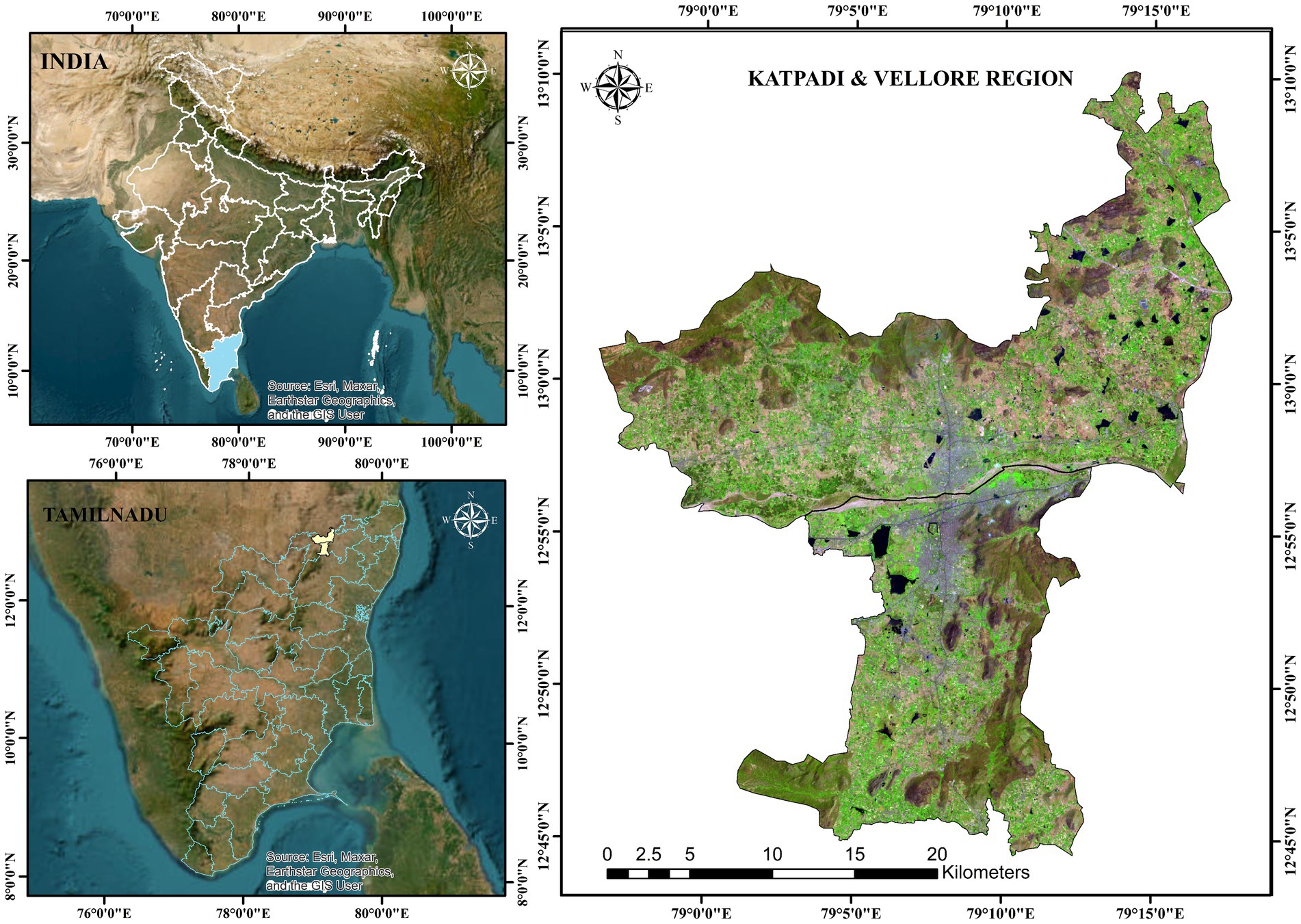
Figure 1. Study area map of Vellore & Katpadi.
Data were collected using publicly available geographic datasets. The primary data source was the United States Geological Survey (USGS). These sites supplied Geo TIFF-format files for 1997, 2005, 2010, 2015, 2020, and 2024. Data accuracy was ensured by using only tiles with 0% cloud cover. Table 1 summarizes the individual satellite datasets used in this study. The methodological flow is depicted in the Supplementary Figure S1.
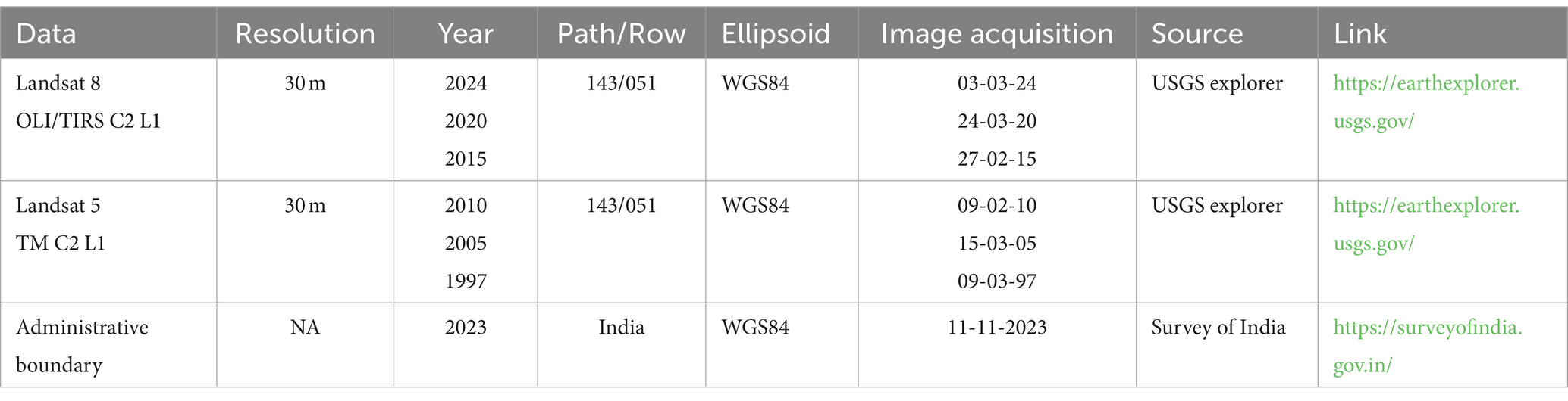
Table 1. Satellite datasets were used in this study.
Land-based classification is an essential element in LULC preparation. Landsat 8 and 5 imagery from the USGS Earth Explorer1 were analyzed using ArcGIS 10.8.2 software for 1997, 2005, 2010, 2015, 2020, and 2024. A supervised image classification strategy using the Support Vector Machine (SVM) algorithm was used to classify LULC into seven categories: water bodies, flooded regions, built-up areas, barren lands, agricultural lands, rangelands, and vegetation. The classification was based on FAO guidelines (Anderson et al., 1976) and FAO standards (FAO, 2000), with statistical information in Supplementary Table S1.
Accuracy assessment is the most significant factor in the reliability of LULC classification. It estimates the precision of LULC maps by comparing the classified results with reference data. In the study, 100 points were randomly selected to prepare the confusion matrix. We employed a comprehensive accuracy assessment framework to calculate the kappa coefficient, overall accuracy, producer’s accuracy, and user’s accuracy in constructing a confusion matrix.
LST was estimated using thermal bands (Bands 10 and 11) from the Landsat series (Rahman et al., 2022). Steps 1 to 6 provide a complete evaluation of the LST for Landsat 8 for 2024, 2020, and 2015. Steps 7 & 8 cover the LST for 2010, 2005, and 1997, respectively (USGS, 2019; EROS, 2020).
Step 1: Earth Radiation Budget (ERB) Radiance for Landsat 8.
The brightness of the Earth’s radiation refers to the surface’s spectral radiance at a specific wavelength. The brightness value is expressed in watts per meter squared per steradian per micrometer.
where:
LλERB = ERB spectral radiance (Watts/(m2 * sr * μm)).
ML = Band-specific multiplicative rescaling factor.
AL = Band-specific additive rescaling factor.
Qcal = Quantized calibrated pixel values (DN).
Oi = Correction value.
Step 2: Calculation of the Top of Atmosphere Brightness Temperature (ABT) Landsat 8.
Thermal data were converted from spectral radiance (Equation 1) to top-of-atmosphere brightness temperature using thermal constant values.
where:
ABT = Top of atmosphere brightness temperature (Kelvin (K) to Celsius (°C)).
K1, K2 = Band-specific thermal conversion constant (Plank’s radiation constant).
Step 3: Calculation of the normalized difference vegetation index (NDVI).
The NDVI is a standardized vegetation index estimated from visible red and NIR bands reflected by greenery.
where:
RED = RED band (ρBand 4).
NIR = Near-infrared band (ρBand 5).
Step 4: Calculation of the land surface emissivity (LSE).
It indicates emissivity from the ground surface and a combination of diverse entities (soil, vegetation, water, rock, and so on). The surface emissivity was calculated from NDVI values of Equation 3 and the greenness of land surfaces (Khan et al., 2022; Sajib and Wang, 2020).
Step 5: Calculation of the surface emissivity “ε”.
where:
ε = Land surface emissivity.
PV = Magnitude of vegetation.
Step 6: Calculation of land surface temperature (LST).
The LST is the ratio of the radiative temperature reflected from a surface to the radiation from an ideal black surface area at a similar temperature. It is retrieved from Equations 2, 4, 5.
where:
λ = Wavelength of emitted radiance.
C2 = Planks radiation constant in mK (milli kelvin).
Step 7: LST Calculation of the Digital Number to Radiance (R) for Landsat 5:
The Landsat 5 dataset with thermal band number 6 was used to determine LST for 1997, 2005, and 2010 (EROS center, 2020).
where:
QCAL = Quantized calibration pixel value in DN.
LMAXλ = Spectral radiance scaled to QCALMAX in Watts/(m2 * sr * μm).
LMINλ = Spectral radiance scaled to QCALMIN in Watts/(m2 * sr * μm).
QCALMIN = Minimum quantized calibrated pixel value in DN.
QCALMAX = Maximum quantized calibrated pixel value in DN.
Step 8: Calculation of Radiance to Brightness Temperature using Equation 7 for a Landsat 5 (USGS and EROS, 2003).
where:
T = Satellite temperature in degrees.
K1, K2 = Calibration constant.
The UHI is calculated using LST (Equations 6, 8) data:
where:
LSTm = The mean temperature of the land surface temperature.
SD = Standard deviation.
Spearman’s coefficient of multivariate correlation was used to assess the correlations between LST and indices such as NDVI, NDBI, NDWI, and MNDWI (Khan et al., 2019; Laerd, 2024). All statistical computations were performed using JMP Pro software and MS Excel (Jmp, 2024). The correlations are represented via scatter plots and color heat maps. Time series analysis and regression coefficients were used to analyze the trend in the interaction effect of WSAs on LST.
The graphical representation of LULC change is shown in Figure 2, illustrating the rise and drop with yearly classified LULC patterns. The summary statistics for the estimated percentage of area trends of each LULC type are shown in Supplementary Table S2.
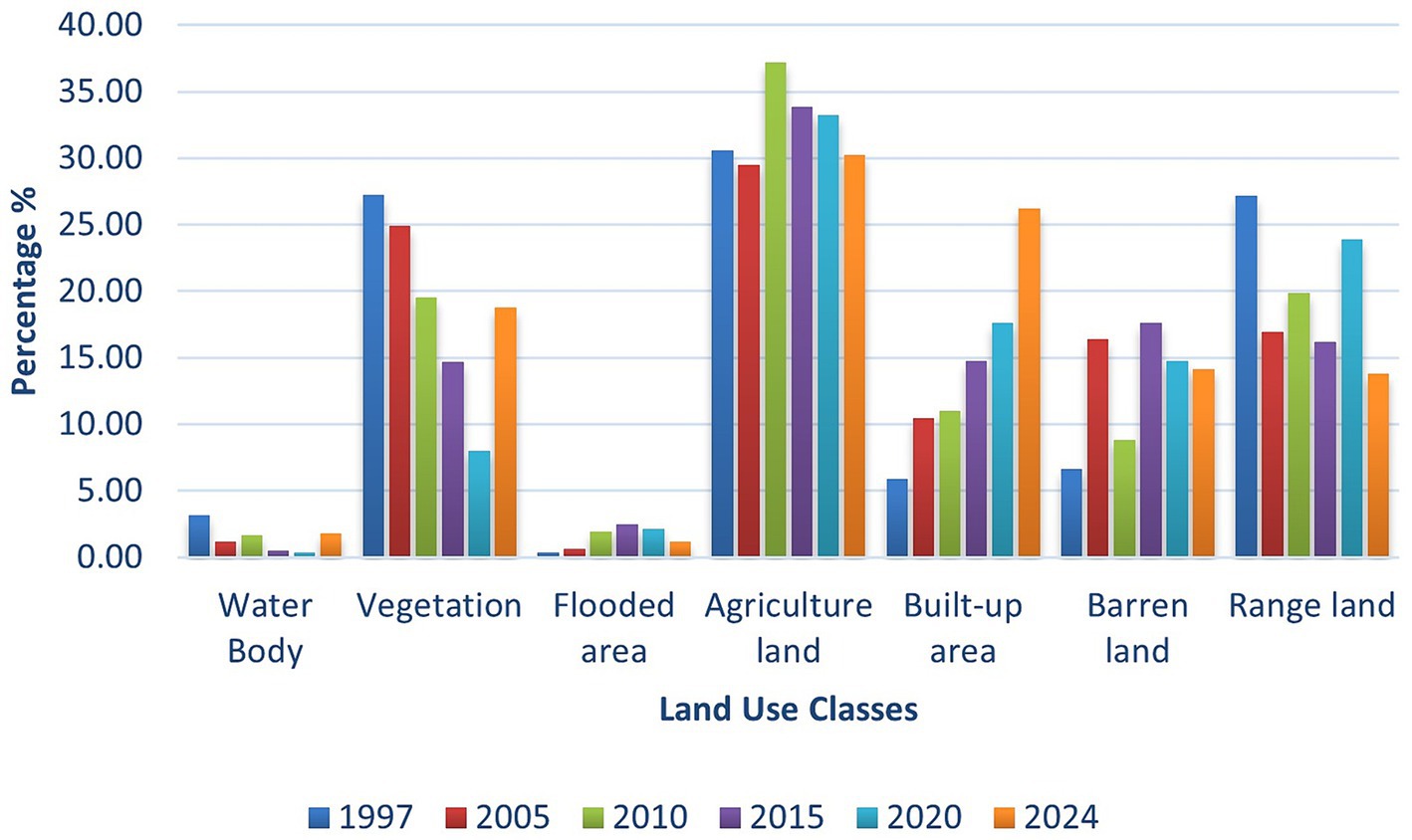
Figure 2. LULC change statistics for all classes from 1997 to 2024.
The LULC classification maps of Vellore and Katpadi for 1997, 2005, 2010, 2015, 2020, and 2024 are given in Figure 3. The overall water bodies reduced from 3.17% in 1997 to 1.12% in 2024, indicating severe water loss. Most of the water-surrounded banks, drylands, and surroundings have diminished. Figure 3 shows the decrease in water bodies in Vellore, especially in the southwest part of Vellore and the northeast parts of Katpadi. Built-up lands increased five times between 1997 and 2024 (Figures 2, 3) as the population increased by 2.30 times, significantly impacting the expansion of built-up areas (UN, 2024). The built-up expansion has progressively increased along the key national highways, along the banks of the Palar River, in the flooded area, and around the region of Vellore & Katpadi.
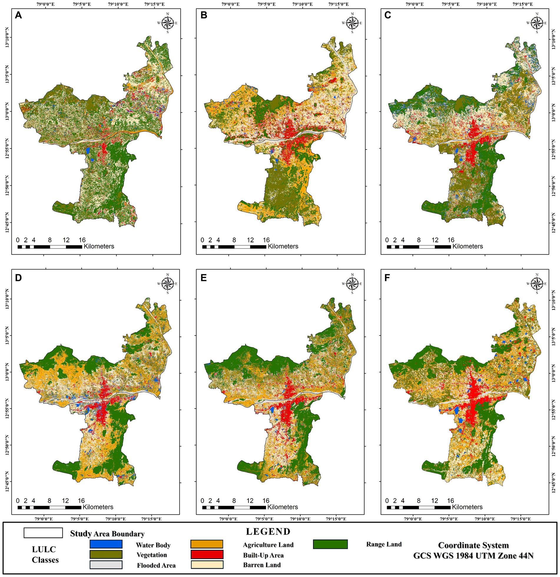
Figure 3. LULC classification of Vellore & Katpadi for (A) 1997, (B) 2005, (C) 2010, (D) 2015, (E) 2020, and (F) 2024.
The agricultural area was 30.57%, and the vegetation was 27.22%, accounting for the most significant proportion of the study area covered in 1997. The conversion of agricultural land to barren land indicates a shift in land use patterns, suggesting a potential change in dependency on seasonal crops or a transition to dryland farming practices. The range dense cover area spotted by 50% decreased from 1997 to 2024 in the southeastern and northern regions, which is not a good sign for natural habitat. The possibility of change in the river belt shows that 3.16% of flooded areas were developed along the banks of the river. The imbalanced mix of pixels can also be seen in all classifications.
Considering all land use classifications, it indicates a significant shift towards urbanization, with a corresponding decline in water bodies and vegetation. Losing water bodies and vegetation cover can exacerbate climate change water quality and reduce air quality and food security. The trend of a rapid expansion of built-up areas can lead to pressure on the ecosystem. The observed changes in vegetation and agriculture changes have confirmed the trends observed by Ghosh and Porchelvan (2010) and Tiwari and Kanchan (2024) These findings must be crafted for sustainable land use practices, potential conservation efforts or land management practices, and climate change.
This accuracy assessment of the LULC maps was conducted using 100 random points. These points were cross-referenced with ground truth points using Google Earth Pro. The assessment involved analyzing producer accuracy and user accuracy with the help of a confusion matrix for individual time periods. The ground truth points were evaluated based on physical observation and Earth Pro data (Kafy et al., 2021b; Rahman et al., 2022; Khan, 2021). The assessment revealed an overall accuracy of 83% in 1997, 73% in 2005, 78% in 2010, 76% in 2015, 83% in 2020, and 92% in 2024. The kappa coefficient values were 0.78, 0.65, 0.72, 0.7, 0.78, and 0.89 for the respective years. The user accuracy was 60–100% for water areas and built-up areas 79.5–100.0%. The result of producer accuracy was above 71% for all classes except flooded areas and vegetation. These results indicate that the accuracy of the LULC maps was above average and of high quality.
The NDVI is said to be a numerical index used to evaluate a region that has live green vegetation using the spectrum ranging from +1 to-1, where values range from-1 to 0 indicate lower green (dry or stressed vegetation), and + 1 indicates denser green vegetation (Cai et al., 2018; Feng et al., 2019).
Figures 4A,B reported the maximum value of 0.9 to 0.6 NDVI range from 1997 to 2005, indicating an area with a good amount of healthy, denser vegetation. Subsequently, values decreased slightly from 0.54 in 2015, 0.55 in 2020, and 0.52 in 2024, proving that vegetation density declined over a period of time (Figure 4).
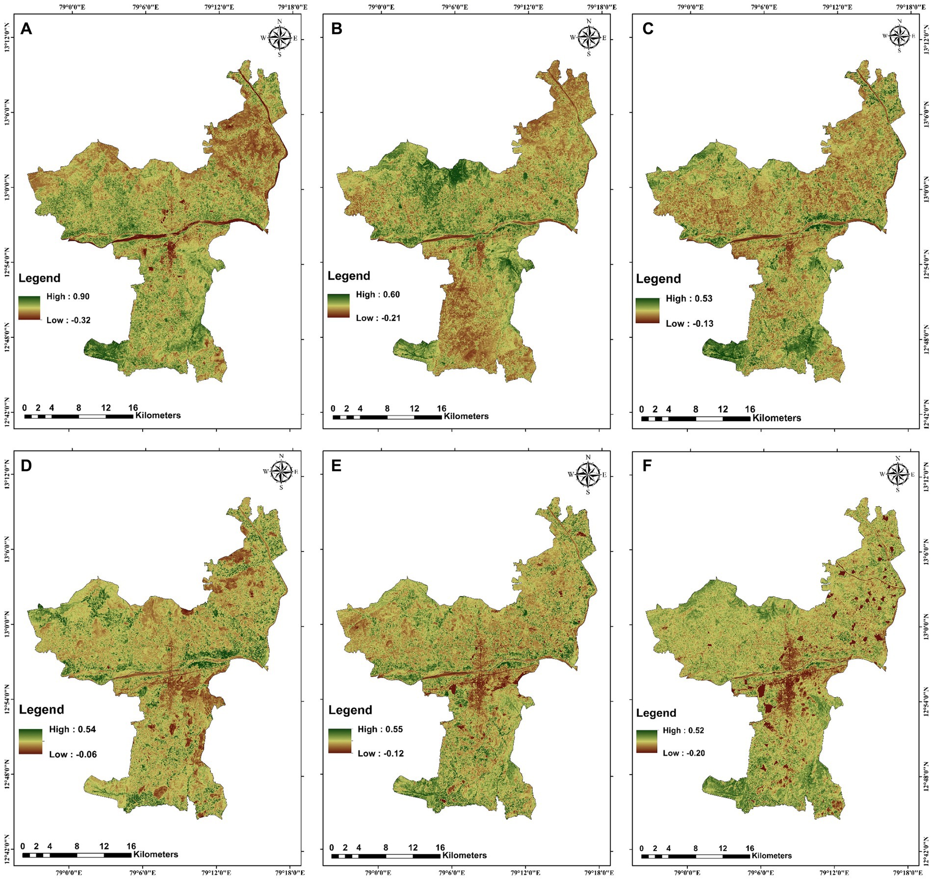
Figure 4. Temporal variation in the normalized difference vegetation index (NDVI) in the study area (A), 1997 (B), 2005 (C), 2010 (D), 2015 (E), 2020, and (F) 2024.
The NDBI is a numerical index used to identify the built-up presence or an artificial structure based on the reflectance of shortwave and near-infrared waves, with values ranging from +1 to-1, where +1 indicates the density of buildings and-1 to 0 indicate the natural features in a region (Addas, 2023; Yang et al., 2023).
Figure 5A shows an NDBI value of 0.34 in 1997, indicating a low density of built-up areas. Figure 5D shows that the maximum value increased to 0.56 in 2015, reflecting a return to a high built-up density. Figure 5F shows a maximum NDBI value of 0.62 in 2024, indicating the changes after the COVID-19 pandemic (Cov-2, 2023). A detailed observation reveals that built-up pixels are generally mixed with barren and agricultural land, with greater differences noted between 2005 and 2015 due to limitations in resolution (Figures 5B,C,E).
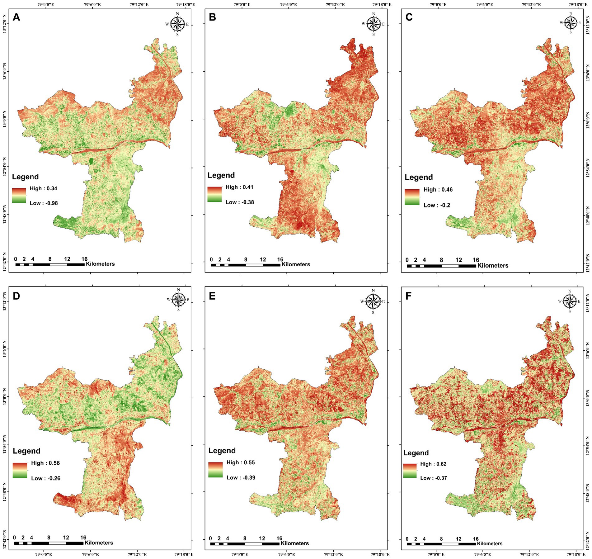
Figure 5. Normalized difference built-up index (NDBI) temporal variation in the study area for (A) 1997, (B) 2005, (C) 2010, (D) 2015, (E) 2020, and (F) 2024.
The NDWI detects water presence by near-infrared absorbance and mid-infrared reflectance. The NDWI value ranges from-1 to +1, with-1 indicating water stress areas and 1 indicating more water pixels or the presence of water bodies (Feng et al., 2019; Tan et al., 2020).
The changes in water bodies over time are represented in Figures 6A,B, with the maximum NDWI range of 0.5 indicating a relatively greater presence of water in 1997. Figure 6F shows an NDWI value of 0.2 in 2024, indicating a small presence of water in the lakes after 2015. The fluctuation of water changes from 1997 to 2024 is verified with the global water occurrence change intensity dataset from 1997 to 2023 (JRC, 2024; Pekel et al., 2016).
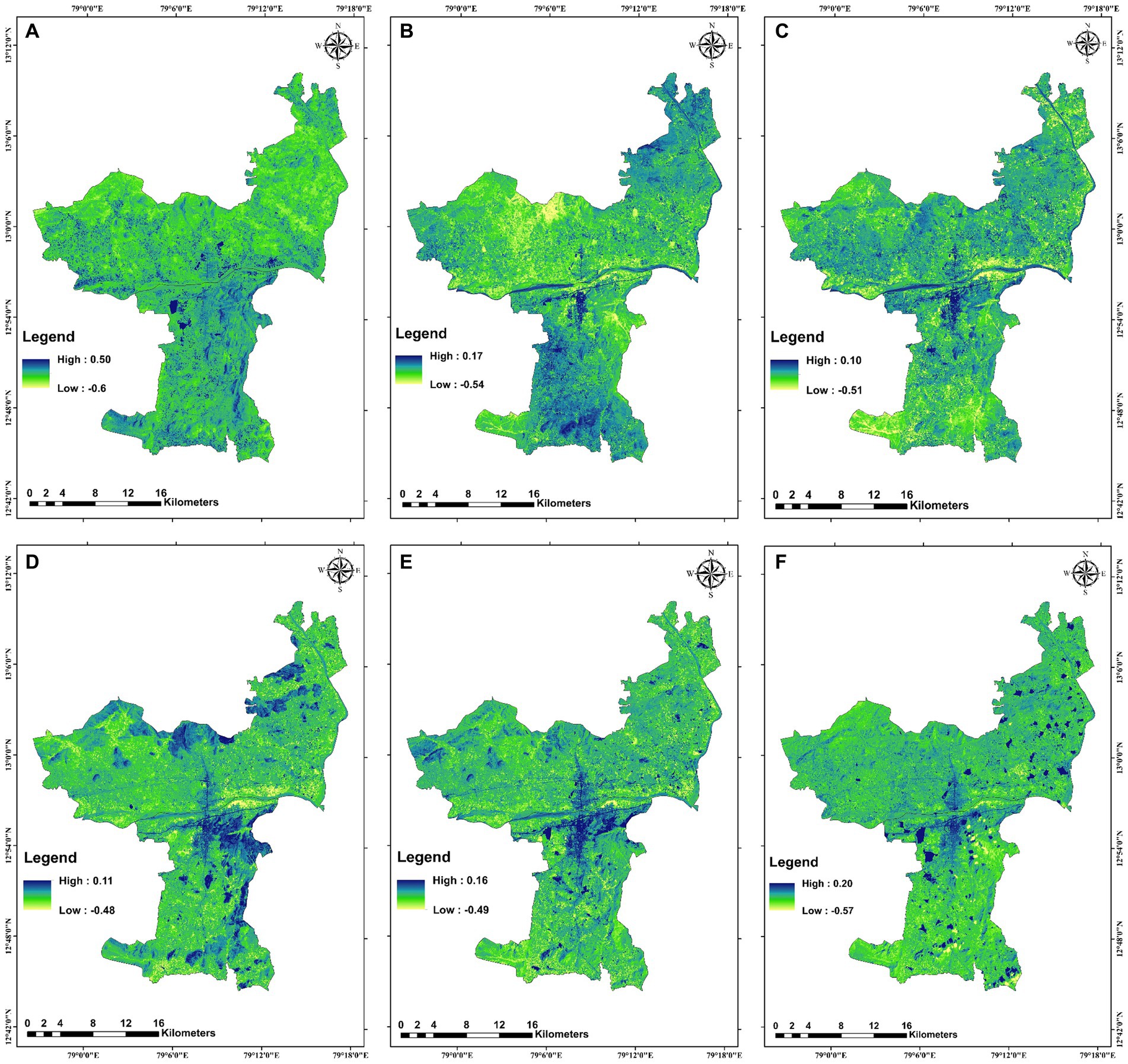
Figure 6. Temporal variations in the normalized difference water index (NDWI) in the study area (A) 1997, (B), 2005, (C) 2010, (D) 2015, (E) 2020, and (F) 2024.
This index is a modification of NDWI, which uses green and shortwave infrared bands to enhance the water concentration. A positive 1 indicates a water feature, whereas zero or negative values imply vegetation or soil (Xu, 2006).
Figure 7A shows that the maximum MNDWI value of 0.49 was moderate in 1997. As a result, the value is reduced to 0.37, which can be absorbed in 2024. The reflectance value shows fewer green pixels surrounding water bodies in lake areas due to the enhancement of the green band.
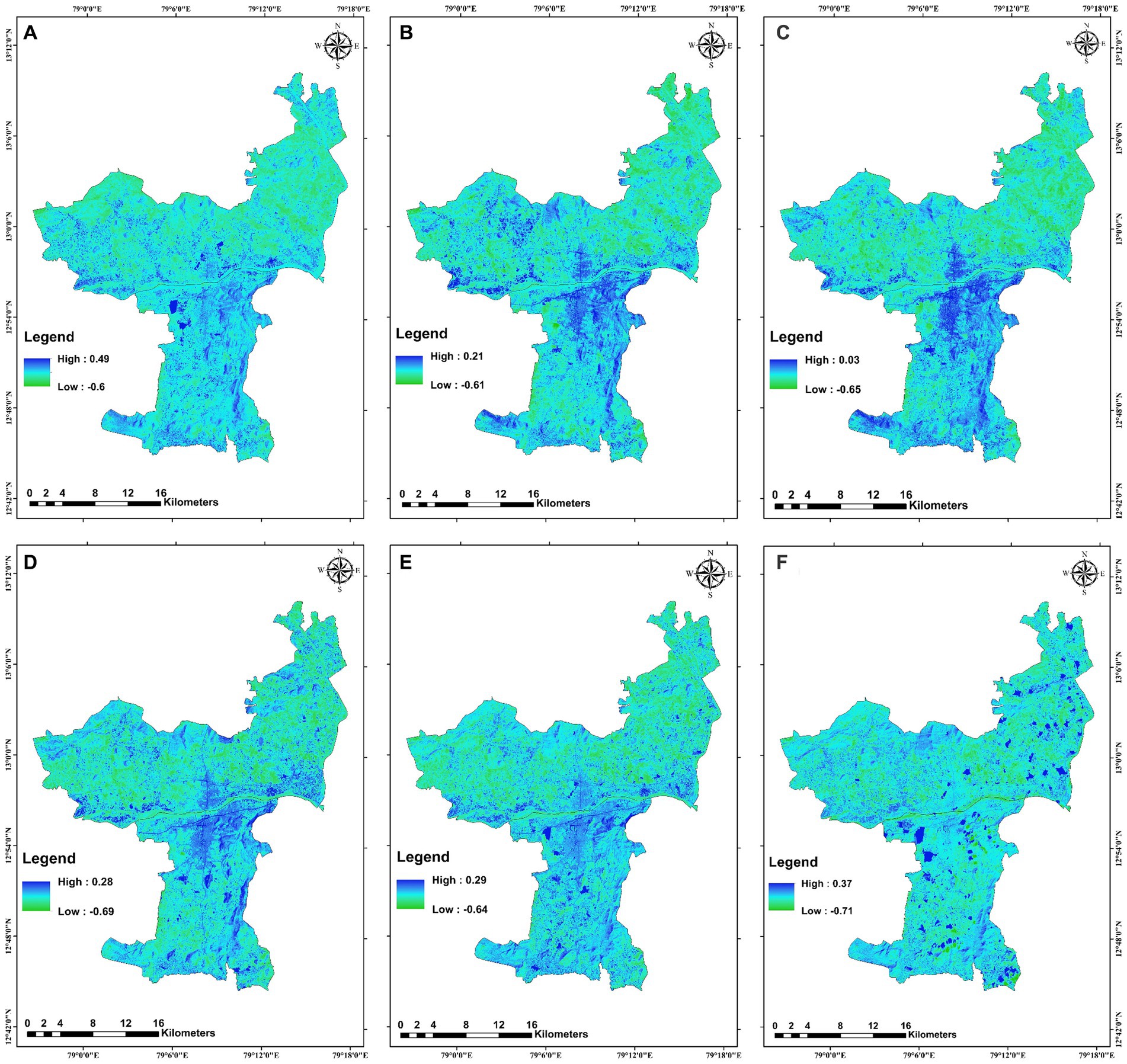
Figure 7. Temporal variation in the modified normalized difference Water index (MNDWI) in the study area (A) 1997, (B) 2005, (C) 2010, (D) 2015, (E) 2020, and (F) 2024.
Thermal sensors are used in LST extraction (Das et al., 2020; Zhao et al., 2023). Various LULC classes were covered: water bodies, vegetation, built-up areas, barren land, dense vegetation, flooded land, and agricultural land. Figure 8 shows the temporal LST patterns for 1997, 2005, 2010, 2015, 2020, and 2024.
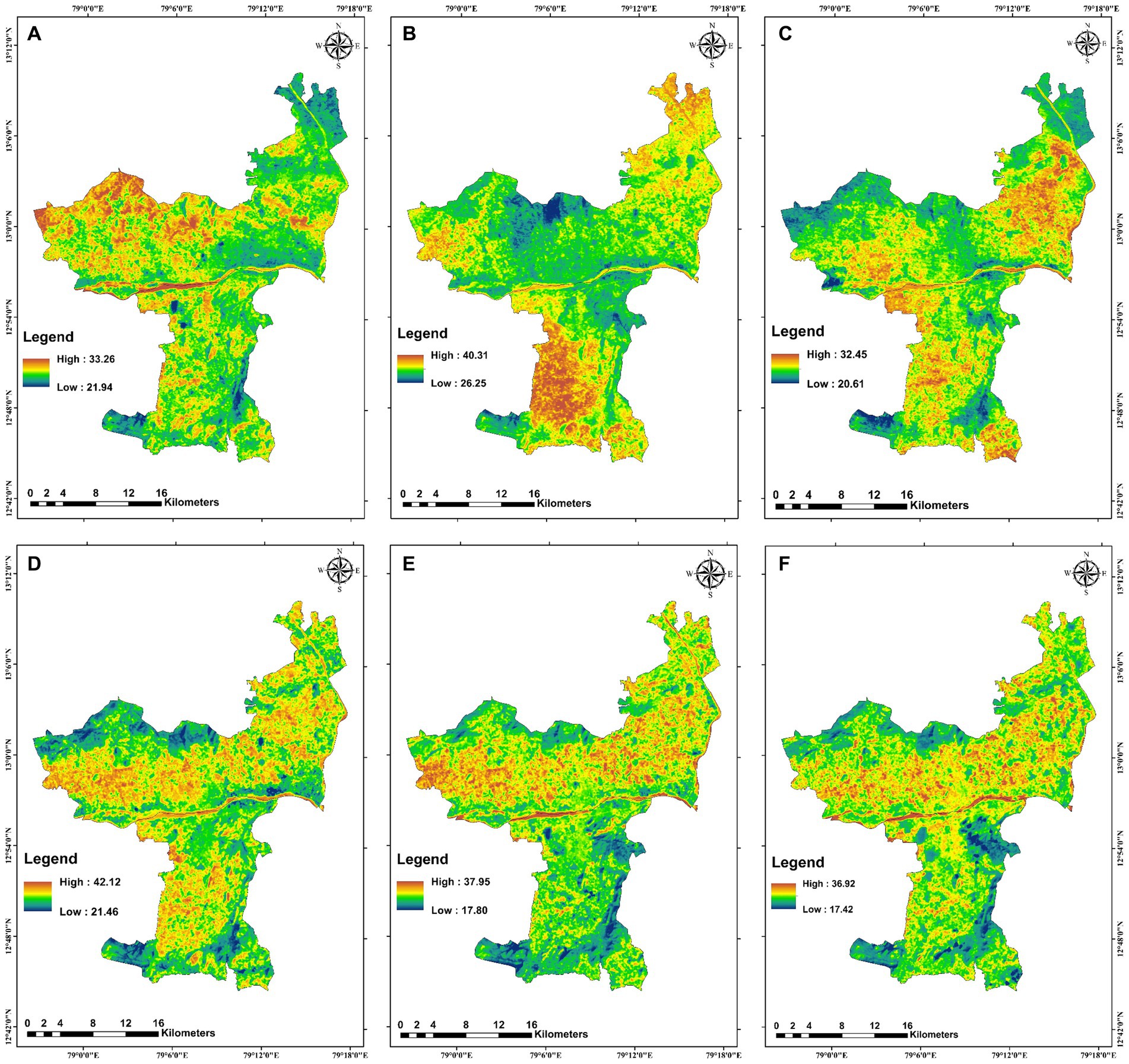
Figure 8. LST spatial–temporal variations in °C (A) 1997, (B) 2005, (C) 2010, (D) 2015, (E) 2020, and (F) 2024.
The LST patterns in Figure 8 show that water bodies and range-dense vegetation cover exhibited lower temperatures ranging from 17.4°C to 26°C. This cooling effect is attributed to the water’s high absorbance and cooling influence on air temperature, commonly referred to as blue spaces (Deng et al., 2018; EPA, 2014; WMP, 2023). Dense vegetation similarly showed lower temperatures due to the process of evapotranspiration. In contrast, barren land and flooded area zones exhibited higher LSTs ranging from 28°C to 42.6°C.
Agricultural lands experienced temperature fluctuations from 20.1°C to 29°C, which can be explained by the variability of seasonal crops and farming practices. Built-up areas showed LSTs ranging from 27.8°C to 42.6°C, which is indicative of the Urban Heat Island (UHI) effect caused by the retention of heat on surfaces. LST results reported in Figure 8 are closely comparable with air temperature data for the years 1997, 2010, 2020, and 2024 are verified with the German Weather Service (DWD) and European Centre for Medium-Range Weather Forecasts (ECMWF) model data (Ventusky n.d.).
Climate change and land use practices have influenced the observed temperatures from 1997 to 2024. A gradual increase in LST during the period highlights the importance of considering regional factors and temporal scales in LULC and LST analyses (Rubeena and Tiwari, 2022; Tiwari and Kanchan, 2024). Notably, the maximum LST values reported for built-up areas in Vellore by Rubeena and Tiwari (2022) closely align with our findings for built-up and barren land. Effective land management strategies focusing on increasing vegetation cover, preserving water bodies, and implementing sustainable urban planning could help mitigate rising temperatures and enhance cooling effects in urban landscapes. Figure 8 reveals a decrease in blue and green areas (representing water and vegetation) and an increase in dark red and light yellow areas, indicating a reduction in vegetation and an associated rise in LSTs.
UHIs were extracted using urban and nonurban LST comparison methods (Feng et al., 2019). Figure 9 shows the spatial distribution of the UHI impact calculated using Equation 9 for 1997, 2005, 2010, 2015, 2020, and 2024. In 1997, the distribution of the UHI impact was significantly less. A temperature drop was also observed, particularly around dense vegetation and water bodies (shown in blue pixels in LST).
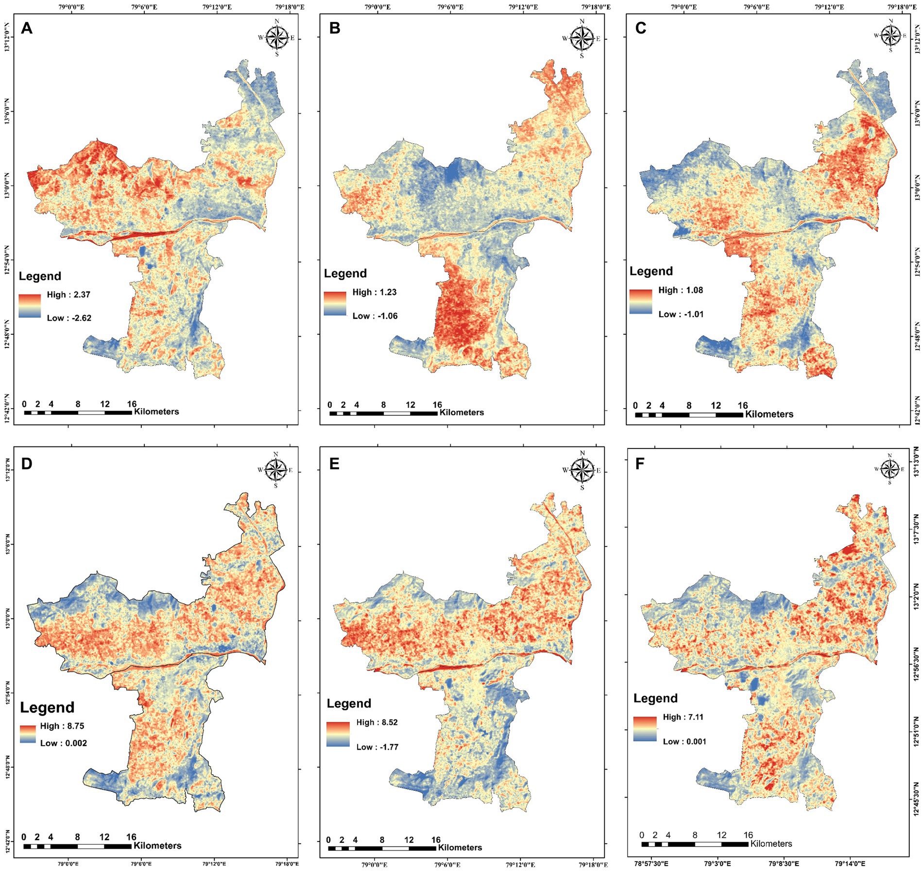
Figure 9. Urban heat intensity (UHI) of temporal patterns in °C (A)1997, (B) 2005, (C) 2010, (D) 2015, (E) 2020, and (F) 2024.
However, from 2005 to 2020, water bodies experienced an increase in the LST, resulting in an influence on the UHI effect, which might be due to the shift of water to other classes. Between 2020 and 2024, the study indicates that the warming trend will vary with rapid urban pointing areas. Unlike the results by Mahata et al. (2024), an increase in UHI and hotspots is observed. Figure 9 shows how UHIs and LSTs influence land cover changes, particularly near built-up areas, water bodies, and dense rangelands. The consistent rate of UHI from 2020 to 2024 may have resulted in post-pandemic adjustments, progressive SDGs (SDG, 2022; SDR, 2022), and smart city missions (SCMG, 2015).
An assessment of the correlation between indices, namely, the NDVI, NDWI, MNDWI, and NDBI, over LST through the integration of a multivariate correlation investigation is needed. The indices were used as independent variables (predictor variables), with the LST as the dependent variable (response variable). Statistical relationships derived from the Landsat series data explorer using JMP Pro.
Following Mustafa et al. (2020), we quantitatively attempted to explain the LST variation by selecting a point over the study area, as shown in Figure 10. Moreover, 100 random points were analyzed while covering all the perspective classes. All georeferenced points (longitude, latitude) and LSTs were decoded with the NDVI, NDBI, NDWI, and MNDWI values extracted using ArcGIS 10.8 from 1997, 2005, 2010, 2015, 2020, and 2024.
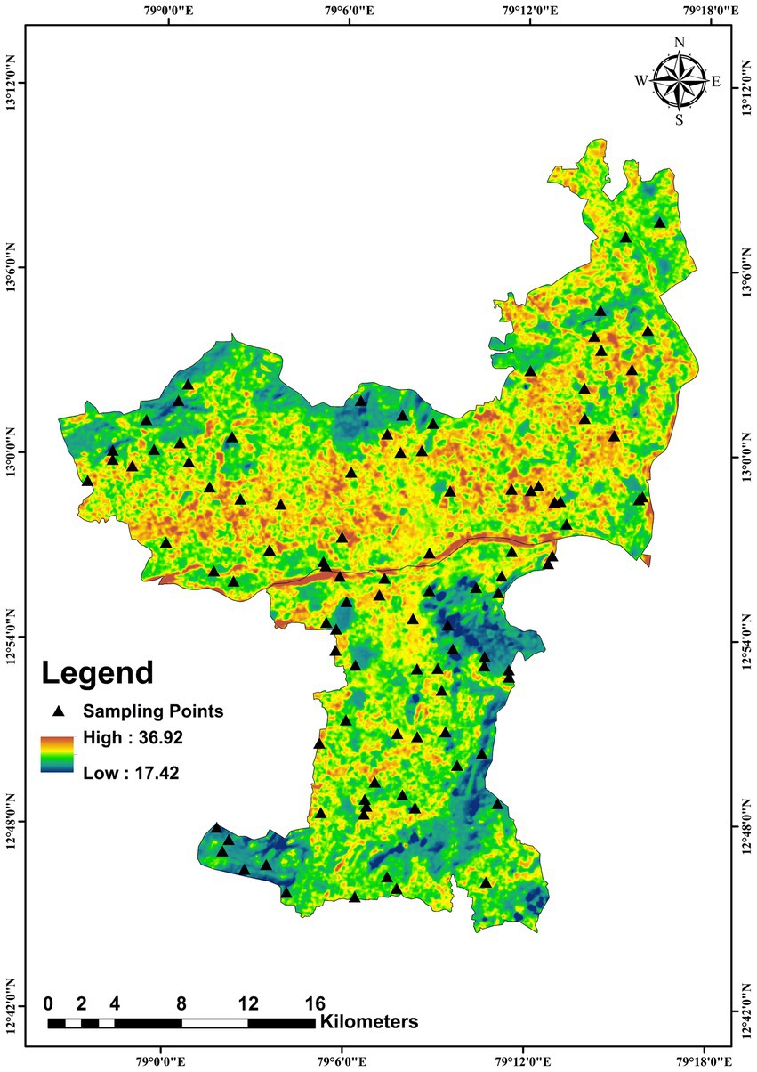
Figure 10. Distribution of sampling points in the study area in °C.
The differences in the LST and subsequent indices (NDVI, NDWI, NDBI, and MNDWI) were examined to determine the dependency of LST. The Spearman’s correlation coefficients were calculated to evaluate the relationships. The scatter plots of the NDVI vs. LST, NDBI vs. LST, NDWI vs. LST, MNDWI vs. LST, NDBI vs. NDVI, and NDBI vs. NDWI are presented in Figure 11, where the assigned correlation attributes are indicated by color plots representing the level of correlation.
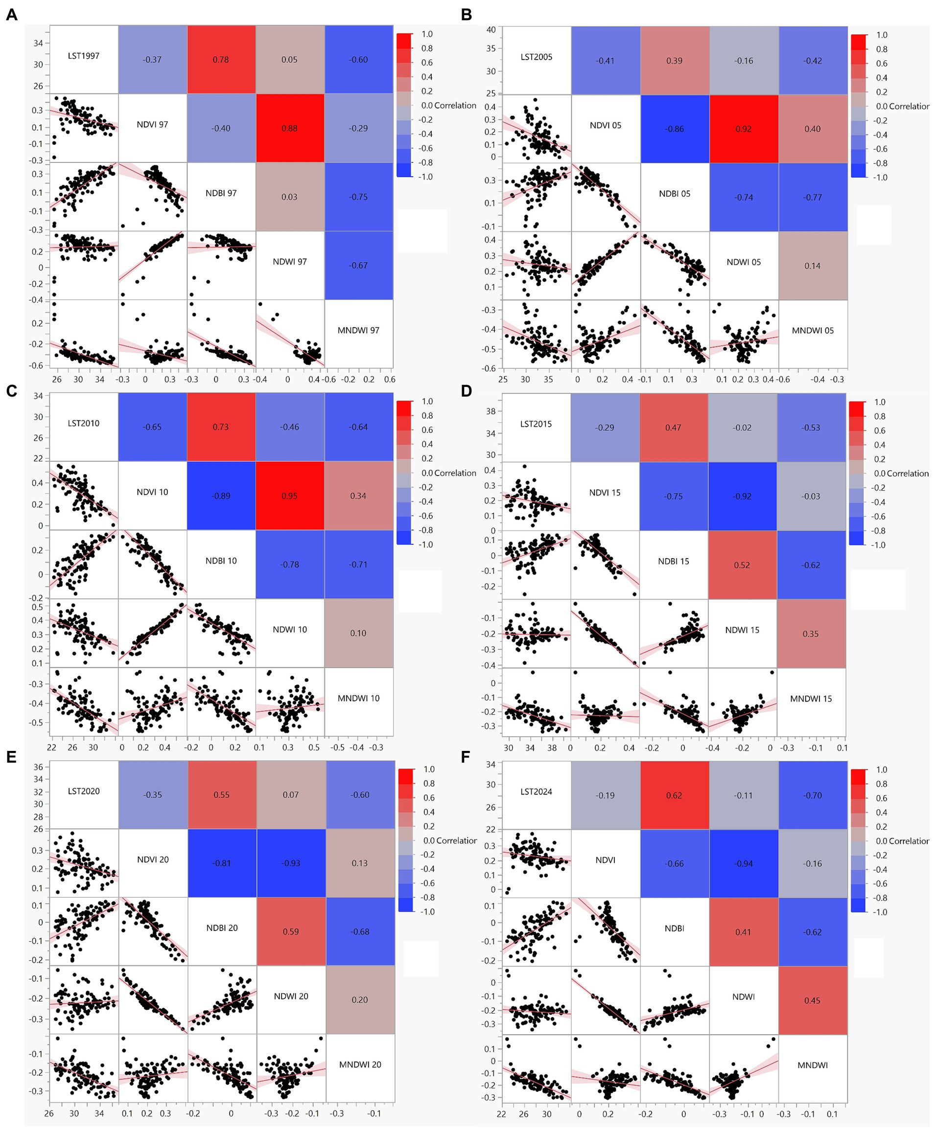
Figure 11. Showing the multivariate correlation indices LST, NDBI, NDVI, NDWI, and MNDWI from (A) 1997, (B) 2005, (C) 2010, (D) 2015, (E) 2020, and (F) 2024.
The monotonic correlation between the NDBI and LST with 95% confidence intervals had Spearman’s ρ values of 0.78 for 1997, 0.39 for 2005, 0.73 for 2010, 0.47 for 2015, 0.55 for 2020, and 0.62 for 2024, respectively, as shown in Figure 11. The aforementioned values indicate a positive relationship between built-up areas and LST. The NDVI and LST correlate with-0.37 for 1995, −0.31 for 2005, −0.65 for 2010, −0.29 for 2015, −0.35 for 2020, and −0.19 for 2024. From 1997 to 2024, reflecting the inverse relationship between NDVI and LST. Similarly, Spearman’s coefficients of the water indices were 0.05 for 1997, −0.16 for 2005, −0.46 for 2010, −0.02 for 2015, 0.07 for 2020, and −0.11 for 2024. These values indicate a variable relationship between water bodies and LST, with some years showing a weak cooling effect. The Spearman’s coefficients of the modified differences water indices were-0.60, −0.42, −0.64, −0.53, −0.60, and −0.70 for years 1997 to 2024. These consistently negative correlations suggest that larger or healthier water bodies will tend to lower land surface temperatures.
The NDVI and NDBI were negatively correlated. The NDVI, NDWI, and MNDWI were strongly correlated from 1997 to 2010 and moderately correlated from 2015 to 2024, reporting the changing influence of LST over time.
Climate change has led to a global decline in water bodies, highlighting the need to investigate the impact of LST on water indices to identify cooling strategies. The gradual shrinkage of lakes is a pressing global issue attributed to both natural factors (humidity, precipitation) and human activities (Zhang et al., 2018; Yang et al., 2023). Figure 12 shows the selected lakes (Saduperi, Kalainjur, Dharapadavedu, and Thorapadi) in Vellore and Katpadi that experienced LST changes. To understand the effect of WSA on regional climate, we conducted a periodic assessment of WSAs and LST spatial variability in the study area from 1997 to 2024. The consistent decline in WSAs in the region is a significant concern, necessitating an assessment to understand changes in WSAs and LST. Figure 13 illustrates the spatial patterns of LULC with the WSA of lakes and their interaction with the LST over the respective years across the study area.
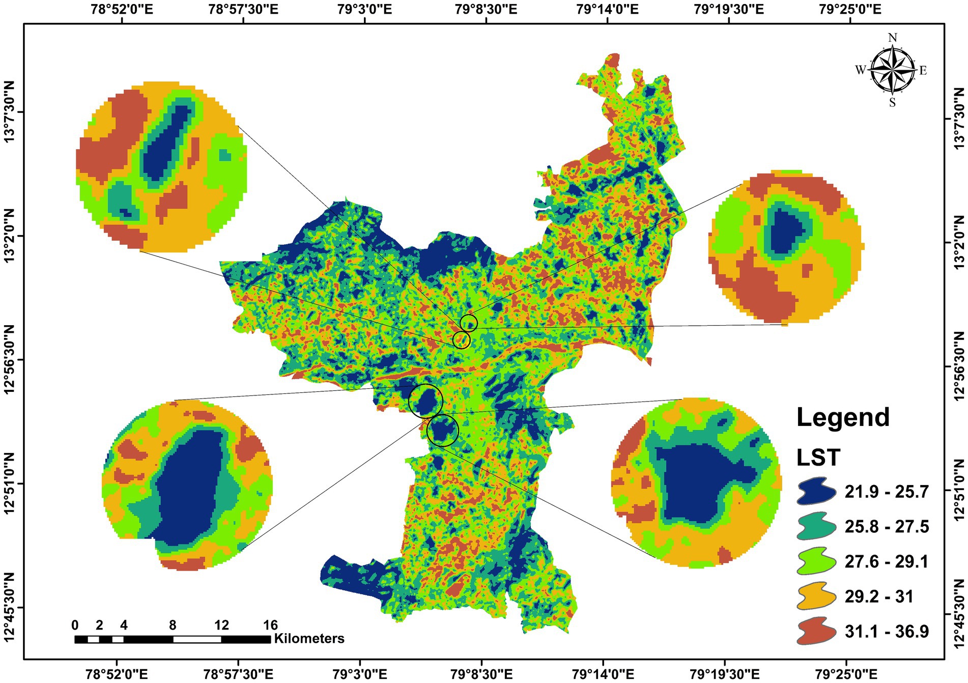
Figure 12. Showing the extracted water body from Vellore & Katpadi experiencing LST°C in 2024.
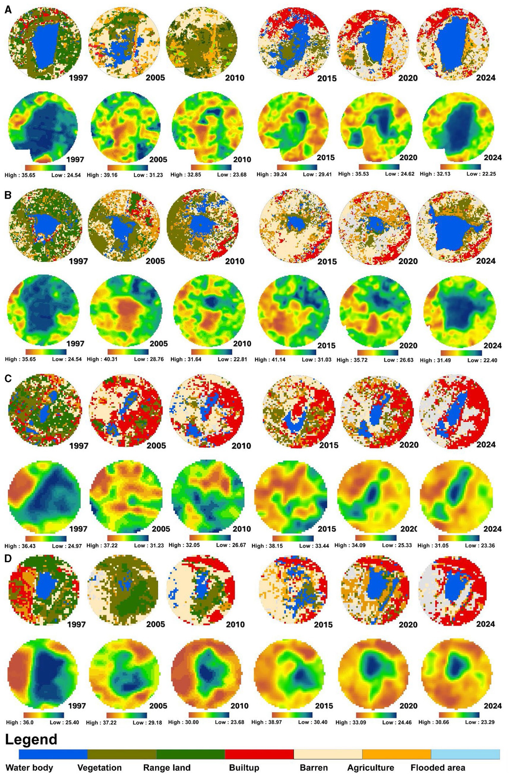
Figure 13. LULC maps of the corresponding LSTs of (A) Saduperi, (B) Thorapadi, (C) Kalinzur, (D) Dharapadavedu Lakes in 1997, 2005, 2010, 2015, 2020, and 2024.
The spatial analysis of LULC and LST for 1997, 2005, 2010, 2015, 2020, and 2024 demonstrates an unpleasant trend in lake degradation, as seen in Figure 13. The WSA started sinking after 1997, followed by a linear decrease from 2005 to 2024. This reflects that the WSAs shift from blue to yellow and red over the time period. This decline is accompanied by an increase in temperature pressure on WSAs, which is evident from the increase in LST, which indicates a strong trend with lake encroachment. Notably, the lakes’ surroundings have transformed from a cooler temperature regime in 1997 to a red, high-temperature zone in 2024, indicating a significant reduction in lake area and increased LST. As a result, the rise in temperature pressure on WSAs is visible, and additional time-series analysis is performed to validate the trend correlation in LST increase in lakes.
Figure 14 shows each lake’s varying time series patterns for LST and WSA. Time series analysis revealed a consistently strong negative correlation between LST and WSA in two of the four lakes. The R2 values indicate the proportion of variation in WSA explained by LST. Specifically, Saduperi Lake (ρ = −0.85, R2 = 0.73) and Dharapadavedu Lake (ρ = −0.95, R2 = 0.91) exhibit strong negative correlations, suggesting a significant inverse relationship between LST and WSA. In contrast, Thorapadi Lake (ρ = −0.20, R2 = 0.04) shows a weak correlation, indicating a negligible relationship between LST and WSA. Kalinzur Lake (ρ = −0.31, R2 = 0.10) displays a moderate negative correlation, suggesting the need for further statistical evidence to clarify their relationship. Factors like humidity, wind speed, size and number of lakes, and dew point can vary yearly, affecting the LST over the WSA. The observed trends support the hypothesis that reduced WSA is associated with increased temperature in two lakes, which is crucial for understanding the climate dynamics and environmental impacts. A scenario-based analysis was conducted to compute the predicted changes in LST under various circumstances by applying the regression equation (Supplementary Equation E1). From regression equations, a 10% reduction in the lake area is likely to result in an average increase in LST of 0.12°C to 0.55°C. Future studies should use high-resolution data and consider additional meteorological and climatic factors, weaker-correlated lakes, and seasonal variations to understand this relationship better.
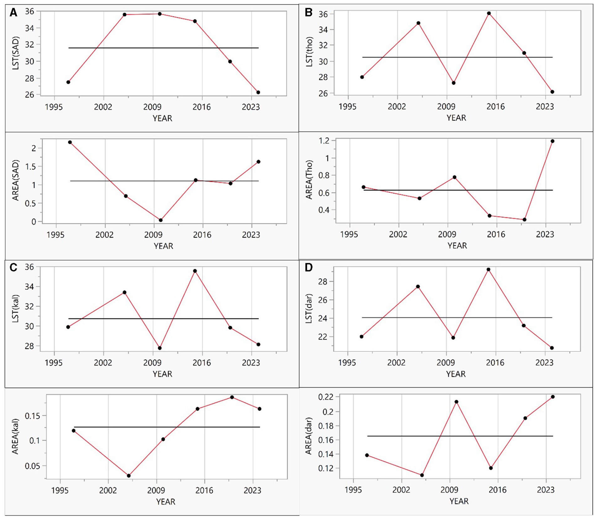
Figure 14. Time series analysis of WSA vs. LST of (A) Saduperi, (B) Thorapadi, (C) Kalinzur, (D) Dharapadavedu lakes.
The impact of Water Spread Areas (WSAs) on rising temperatures highlights the need for strategic ecological space planning. The study area, sensitive to climate change, is subject to direct UV radiation, variable wind patterns, and unique geographical factors, such as elevation and its landlocked position. These factors, coupled with global climate change and urbanization, contribute to fluctuating heat intensity in Vellore. The diminishing role of water bodies and the reduction in dense vegetation cover further emphasize the urgent need for climate-resilient urban planning. The aforementioned discussion gist is represented in Figure 15.
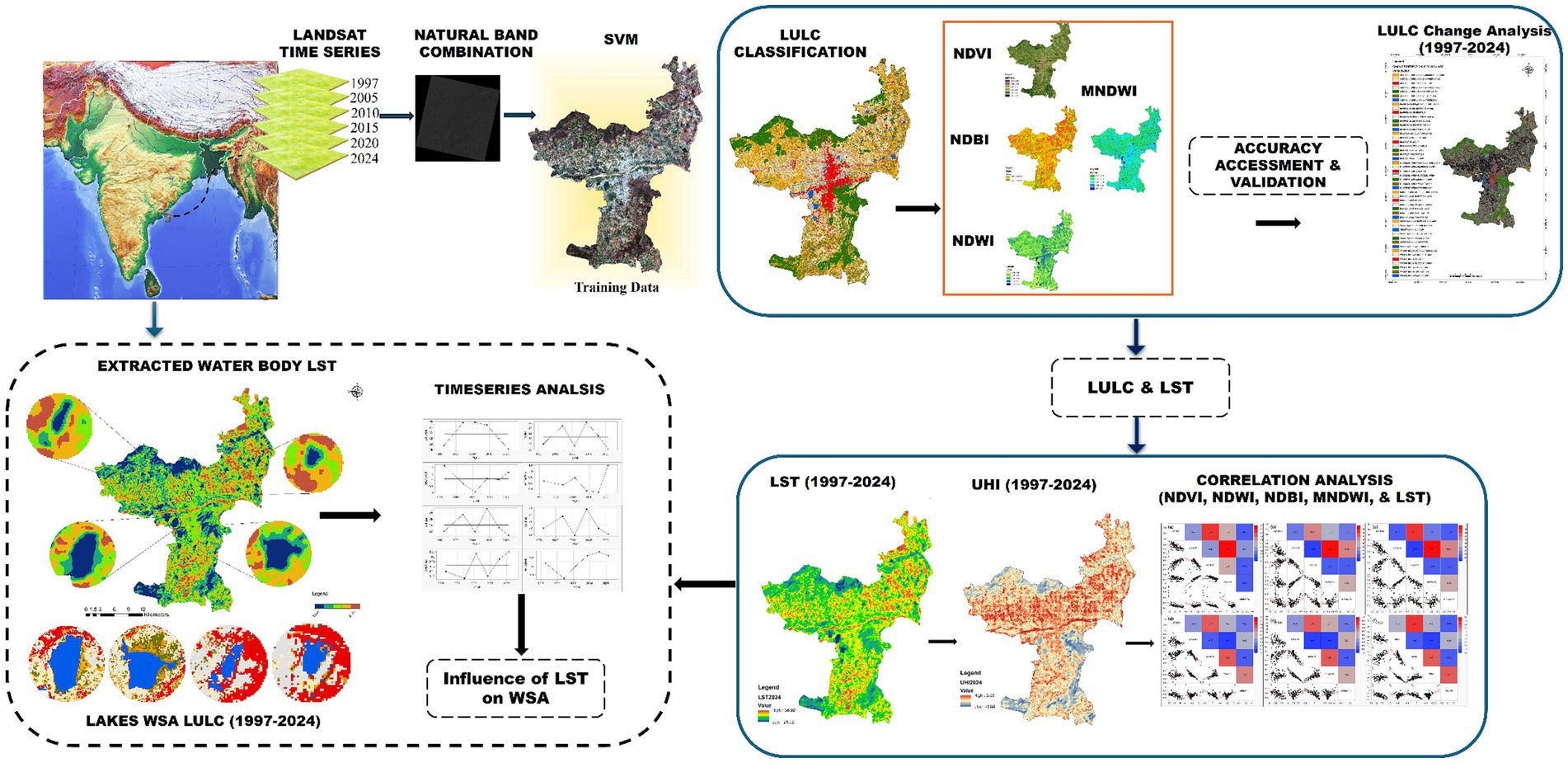
Figure 15. Graphical Abstract - Discussion Gist.
The current study revealed that the interaction between LULC patterns and LST changes, with a particular focus on their impact on water bodies. The study identified significant transformations in land categories over nearly three decades, including an increase in built-up areas, a reduction in vegetation, a decrease in water bodies, and dense rangelands. Additionally, the study observed a reduction in dense vegetation as a result of expanding built-up areas. Supporting these findings, a strong positive correlation was found between LST and NDBI, while negative correlations were observed between NDVI, NDWI, and MNDWI. This indicates notable increases in LST corresponding to decreases in vegetation, water indices, and other natural factors.
The majority of lakes experienced a 10% reduction in area, leading to an average LST increase of 0.12°C to 0.55°C, with a consistent temperature rise over the years. As evident from the analysis, the reduction in water spread area has significantly impacted thermal distribution, primarily due to global warming. These findings carry important implications for urban planning and water resource management, emphasizing the urgent need to conserve and protect water bodies to mitigate the effects of global warming. To address the impact of LULC changes and global warming on water bodies, we recommend the following:
• Implementing zoning regulations to protect lake shorelines and surrounding wetlands.
• Creating new water bodies and restoring degraded wetlands in the region.
• Educating local communities about the importance of water conservation and sustainable land use practices.
• Investing in climate-resilient infrastructure, such as green roofs and permeable pavements, in urban areas surrounding the lakes of Vellore.
• Supporting ongoing research and monitoring of land use changes and water quality in the lakes.
The original contributions presented in the study are included in the article/Supplementary material, further inquiries can be directed to the corresponding author.
DM: Formal analysis, Resources, Software, Writing – original draft, Writing – review & editing. PJ: Conceptualization, Investigation, Supervision, Validation, Writing – review & editing.
The author(s) declare that no financial support was received for the research, authorship, and/or publication of this article.
The authors thank the Vellore Institute of Technology, Vellore, for providing research facilities for conducting this research work.
The authors declare that the research was conducted in the absence of any commercial or financial relationships that could be construed as a potential conflict of interest.
All claims expressed in this article are solely those of the authors and do not necessarily represent those of their affiliated organizations, or those of the publisher, the editors and the reviewers. Any product that may be evaluated in this article, or claim that may be made by its manufacturer, is not guaranteed or endorsed by the publisher.
The Supplementary material for this article can be found online at: https://www.frontiersin.org/articles/10.3389/frsc.2024.1462092/full#supplementary-material
Addas, A. (2023). Machine learning techniques to map the impact of urban Heat Island: investigating the City of Jeddah. Land 12:1159. doi: 10.3390/land12061159
Ahmed, M., Aloshan, M. A., Mohammed, W., Mesbah, E., Alsaleh, N. A., and Elghonaimy, I. (2024). Characterizing land surface temperature (LST) through remote sensing data for small-scale urban development projects in the Gulf cooperation council (GCC). MDPI (Basel, Switzerland: Preprints.Org).
Al Shawabkeh, R., AlHaddad, M., Al-Hawwari, L., Al-Hawwari, M. I., Omoush, A., and Arar, M. (2024). Modeling the impact of urban land cover features and changes on the land surface temperature (LST): the case of Jordan. Ain Shams Eng. J. 15:102359. doi: 10.1016/j.asej.2023.102359
Anderson, J. R., Hardy, E. E., Roach, J. T., and Witmer, R. E. (1976). “A land use and land cover classification system for use with remote sensor data. Reston, VA, USA: US Geological Survey (USGS).
Bagyaraj, M., Senapathi, V., Karthikeyan, S., Chung, S. Y., Khatibi, R., Nadiri, A. A., et al. (2023). A study of urban Heat Island effects using remote sensing and GIS techniques in Kancheepuram, Tamil Nadu, India. Urban Clim. 51:101597. doi: 10.1016/j.uclim.2023.101597
Bayode, T., and Siegmund, A. (2024). Tripartite relationship of urban planning, City growth, and health for sustainable development in Akure Nigeria. Front. Sustain. Cities 5:1301397. doi: 10.3389/frsc.2023.1301397
Beck, H. E., Zimmermann, N. E., McVicar, T. R., Vergopolan, N., Berg, A., and Wood, E. F. (2018). Present and future Köppen-Geiger climate classification maps at 1-km resolution. Sci. Data 5:180214. doi: 10.1038/sdata.2018.214
Bhagat, S., and Prasad, P. R. C. (2024). Assessing the impact of Spatio-temporal land use and land cover changes on land surface temperature, with a major emphasis on mining activities in the state of Chhattisgarh, India. Spat. Inf. Res. 32, 339–355. doi: 10.1007/s41324-023-00563-9
Cai, Z., Han, G., and Chen, M. (2018). Do water bodies play an important role in the relationship between urban form and land surface temperature? Sustain. Cities Soc. 39, 487–498. doi: 10.1016/j.scs.2018.02.033
CMC. (n.d.) “CMC.” Available at: https://www.Cmch-Vellore.Edu/.
Cov-2 (2023). Coronavirus disease (COVID-19) : World Health Organization Available at: https://www.who.int/health-topics/coronavirus?_pan_ssl=Yes#tab=tab_1.
Das, D. N., Chakraborti, S., Saha, G., Banerjee, A., and Singh, D. (2020). Analysing the dynamic relationship of land surface temperature and Landuse pattern: a City level analysis of two climatic regions in India. City Environ. Interact. 8:100046. doi: 10.1016/j.cacint.2020.100046
Das, B., Khan, F., and Mohammad, P. (2023). Impact of urban sprawl on change of environment and consequences. Environ. Sci. Pollut. Res. 30, 106894–106897. doi: 10.1007/s11356-023-29192-3
Deccan Chronicle (2019). Tamil Nadu to be Most urbanized state by 2030 : DC Corrospondent Available at: https://www.deccanchronicle.com/nation/current-affairs/040717/tamil-nadu-to-be-most-urbanised-state-by-2030.html.
Deng, Y., Wang, S., Bai, X., Tian, Y., Luhua, W., Xiao, J., et al. (2018). Relationship among land surface temperature and LUCC, NDVI in typical karst area. Sci. Rep. 8, 1–12. doi: 10.1038/s41598-017-19088-x
Du, H., Song, X., Jiang, H., Kan, Z., Wang, Z., and Cai, Y. (2016). Research on the Cooling Island effects of water body: a case study of Shanghai, China. Ecol. Indic. 67, 31–38. doi: 10.1016/j.ecolind.2016.02.040
EPA (2014). Action that could reduce water temperature : Climate Ready Esturaines Available at: https://www.epa.gov/cre/actions-could-reduce-water-temperature.
EROS (2020). USGS EROS archive – Landsat archives – Landsat 8-9 OLI/TIRS collection 2 Level-2 science products. Sioux Falls, SD, USA: USGS Science of Changing World.
EROS center (2020). USGS EROS archive – Landsat archives – Landsat 4–5 TM collection 2 Level-2 science products. Sioux Falls, SD, USA: USGS Science of Changing World.
Fallmann, J., Forkel, R., and Emeis, S. (2016). Secondary effects of urban Heat Island mitigation measures on air quality. Atmos. Environ. 125, 199–211. doi: 10.1016/j.atmosenv.2015.10.094
FAODi Gregorio, A. (2000). Land cover classification system (Lccs). Nairobi, Kenia Available at: https://www.fao.org/3/x0596e/x0596e00.htm.
Faragallah, R. N., and Ragheb, R. A. (2022). Evaluation of thermal comfort and urban Heat Island through cool paving materials using ENVI-met. Ain Shams Eng. J. 13:101609. doi: 10.1016/j.asej.2021.10.004
Feng, Y., Gao, C., Tong, X., Chen, S., Lei, Z., and Wang, J. (2019). Spatial patterns of land surface temperature and their influencing factors: a case study in Suzhou, China. Remote Sens. 11:182. doi: 10.3390/rs11020182
Ghosh, J., and Porchelvan, P. (2010). “Multi-temporal satellite image and GIS based assessment of urban Landuse changes in Vellore City, Tamilnadu ”. www.IndianJournals.com.
Ghosh, J., and Porchelvan, P. (2018). Relationship between surface temperature and land cover types using thermal infrared band and NDVI for Vellore District, Tamilnadu, India. Nat. Environ. Pollut. Technol. 17, 611–617. Available at: www.neptjournal.com
Govt. of India. (n.d.) “Ministry of earth science.” Available at: https://www.moes.gov.in/documents/annual-reports.
Hsu, A., Sheriff, G., Chakraborty, T., and Manya, D. (2021). Disproportionate exposure to urban Heat Island intensity across major US cities. Nat. Commun. 12:2721. doi: 10.1038/s41467-021-22799-5
IIRS, ISRO. (2017). “Land surface temperature studies in urban areas.” Available at: https://youtu.be/U3u66DKW-vc?si=Zo4RZOSi6vFgJSiu.
IRIS Cheng (2021). The importance of smart cities in the fight against climate change : Global Commons Earth Org. Available at: https://earth.org/smart-cities-climate-change/.
Jain, M. (2023). Two decades of nighttime surface urban Heat Island intensity analysis over nine major populated cities of India and implications for heat stress. Front. Sustain. Cities 5:1084573. doi: 10.3389/frsc.2023.1084573
Jeppesen, E., Meerhoff, M., Davidson, T. A., Trolle, D., Søndergaard, M., Lauridsen, T. L., et al. (2014). Climate change impacts on lakes: an integrated ecological perspective based on a multi-faceted approach, with special focus on Shallow Lakes. J. Limnol. 73, 88–111. doi: 10.4081/jlimnol.2014.844
Jmp (2024). Jmp Stastical discovery : JMP. Available at: https://www.jmp.com/en_us/home.html.
JRC (2024). Water occurrence change intensity (1984-1999 to 2000-2021) global surface water explorer : Joint Research Centre. Available at: https://global-surface-water.appspot.com/download.
Kafy, A. A., Dey, N. N., Al Rakib, A., Rahaman, Z. A., Nasher, N. R., and Bhatt, A. (2021a). Modeling the relationship between land use/land cover and land surface temperature in Dhaka, Bangladesh using CA-ANN algorithm. Environ. Chall. 4:100190. doi: 10.1016/j.envc.2021.100190
Kafy, A. A., Shuvo, R. M., Naim, M. N., Sikdar, M. S., Chowdhury, R. R., Islam, M. A., et al. (2021b). Remote sensing approach to simulate the land use/land cover and seasonal land surface temperature change using machine learning algorithms in a fastest-growing megacity of Bangladesh. Remote Sens. Appl. 21:100463. doi: 10.1016/j.rsase.2020.100463
Khan, F. (2021). Land use classification and land cover assessment using accuracy matrix for Dhamtari District, Chhattisgarh, India. Suranaree J. Sci. Technol. 29, 1–8. Available at: https://www.researchgate.net/publication/361666631
Khan, F., Das, B., and Mishra, R. K. (2022). An automated land surface temperature modelling tool box designed using spatial technique for ArcGIS. Earth Sci. Inf. 15, 725–733. doi: 10.1007/s12145-021-00722-2
Khan, F., Das, B., Mishra, R. K., and Patel, B. (2021). Analysis of land use land cover changes with land surface temperature using spatial-temporal data for Nagpur City, India. J. Landsc. Ecol. 14, 52–64. doi: 10.2478/jlecol-2021-0017
Khan, N., Shahid, S., Chung, E.-S., Kim, S., and Ali, R. (2019). Influence of surface water bodies on the land surface temperature of Bangladesh. Sustainability 11:6754. doi: 10.3390/su11236754
Köppen, W. (n.d.). Köppen climate classification : Wikipedia the free encyclopedia Available at: https://en.Wikipedia.Org/wiki/K%C3%B6ppen_climate_classification.
Laerd (2024). Spearman’s rank-order correlation using SPSS Stastics : Leard Stastics Available at: https://statistics.laerd.com/spss-tutorials/spearmans-rank-order-correlation-using-spss-statistics.php.
Li, J., Li, L., Song, Y., Chen, J., Wang, Z., Bao, Y., et al. (2023). A robust large-scale surface water mapping framework with high spatiotemporal resolution based on the fusion of multi-source remote sensing data. Int. J. Appl. Earth Obs. Geoinf. 118:103288. doi: 10.1016/j.jag.2023.103288
Li, C., Linlin, L., Zongtang, F., Sun, R., Pan, L., Han, L., et al. (2022). Diverse cooling effects of green space on urban Heat Island in tropical megacities. Front. Environ. Sci. 10:1073914. doi: 10.3389/fenvs.2022.1073914
Lin, Y., Wang, Z., Jim, C. Y., Li, J., Deng, J., and Liu, J. (2020). Water as an urban heat sink: blue infrastructure alleviates urban Heat Island effect in Mega-City agglomeration. J. Clean. Prod. 262:121411. doi: 10.1016/j.jclepro.2020.121411
Mahata, B., Sahu, S. S., Sardar, A., Laxmikanta, R., and Maity, M. (2024). Spatiotemporal dynamics of land use/land cover (LULC) changes and its impact on land surface temperature: a case study in new town Kolkata, eastern India. Reg. Sustain. 5:100138. doi: 10.1016/j.regsus.2024.100138
Makumbura, R. K., Samarasinghe, J., and Rathnayake, U. (2022). Multidecadal land use patterns and land surface temperature variation in Sri Lanka.” edited by Maman Turjaman. Appl. Environ. Soil Sci. 2022, 1–11. doi: 10.1155/2022/2796637
Malarvizhi, K., Kumar, S. V., and Porchelvan, P. (2022). Urban sprawl modelling and prediction using regression and seasonal ARIMA: a case study for Vellore, India. Model. Earth Syst. Environ. 8, 1597–1615. doi: 10.1007/s40808-021-01170-z
Murakawa, S., Sekine, T., Narita, K.-i., and Nishina, D. (1991). Study of the effects of a river on the thermal environment in an urban area. Energ. Buildings 16, 993–1001. doi: 10.1016/0378-7788(91)90094-J
Mustafa, E. K., Co, Y., Liu, G., Kaloop, M. R., Beshr, A. A., Zarzoura, F., et al. (2020). Study for predicting land surface temperature (LST) using Landsat data: a comparison of four algorithms. Adv. Civ. Eng. 2020, 1–16. doi: 10.1155/2020/7363546
Mustafa, M. T., Hassoon, K. I., Hassan, M., and Abd, M. H. (2017). Using water indices (NDWI, MNDWI, NDMI, WRI and AWEI) to detect physical and chemical parameters by apply remote sensing and GIS techniques. Int. J. Res. Granthaalayah 55, 117–128. doi: 10.5281/zenodo.1040209
Ninan, G. A., Gunasekaran, K., Jayakaran, J. A. J., Jacob Johnson, K. P., Abhilash, P., Pichamuthu, K., et al. (2020). Heat-related illness—clinical profile and predictors of outcome from a healthcare Center in South India. J. Family Med. Prim. Care 9, 4210–4215. doi: 10.4103/jfmpc.jfmpc_690_20
NOAA. (2024). “Global climate report for February 2024.” Available at: https://www.climate.gov/news-features/understanding-climate/global-climate-report-february-2024.
Pekel, J.-F., Cottam, A., Gorelick, N., and Belward, A. S. (2016). High-resolution mapping of global surface water and its long-term changes. Nature 540, 418–422. doi: 10.1038/nature20584
Piracha, A., and Chaudhary, M. T. (2022). Urban air pollution, urban Heat Island and human health: a review of the literature. Sustainability 14:9234. doi: 10.3390/su14159234
Rahman, M., Naimur, M., Rony, R. H., Jannat, F. A., Pal, S. C., Saiful Islam, M., et al. (2022). Impact of urbanization on urban Heat Island intensity in major districts of Bangladesh using remote sensing and geo-spatial tools. Climate 10:3. doi: 10.3390/cli10010003
Reavilious, K. (2024). Many of World’s lakes are vanishing and some may be gone forever : Newscientist Available at: https://www.newscientist.com/article/2079562-many-of-worlds-lakes-are-vanishing-and-some-may-be-gone-forever/.
Rubeena, V., and Tiwari, K. (2022). Analysis of land use and land cover changes and their impact on temperature using Landsat satellite imageries. Environ. Dev. Sustain. 25, 8623–8650. doi: 10.1007/s10668-022-02416-1
Saha, J., Ria, S. S., Sultana, J., Shima, U. A., Seyam, M. M. H., and Rahman, M. M. (2024). Assessing seasonal dynamics of land surface temperature (LST) and land use land cover (LULC) in Bhairab, Kishoreganj, Bangladesh: a geospatial analysis from 2008 to 2023. Case Stud. Chem. Environ. Eng. 9:100560. doi: 10.1016/j.cscee.2023.100560
Sajib, M. Q. U., and Wang, T. (2020). Estimation of land surface temperature in an agricultural region of Bangladesh from Landsat 8: Intercomparison of four algorithms. Sensors 20:1778. doi: 10.3390/s20061778
Santhosh, L. G., and Shilpa, D. N. (2023). Assessment of LULC change dynamics and its relationship with LST and spectral indices in a rural area of Bengaluru District, Karnataka India. Remote Sens. Appl. 29:100886. doi: 10.1016/j.rsase.2022.100886
SCMG (2015). Smart City Mission guidelines. India Available at: https://smartcities.gov.in/sites/default/files/SmartCityGuidelines.pdf.
SDG (2022). Sustainable development goals. United Nations Available at: https://unstats.un.org/sdgs/report/2022/.
SDR (2022). Sustainable development report : SDG Index & Dashboards Available at: https://dashboards.sdgindex.org/rankings.
Tan, J., De, Y., Li, Q., Tan, X., and Zhou, W. (2020). Spatial relationship between land-use/land-cover change and land surface temperature in the Dongting Lake area, China. Sci. Rep. 10, 1–9. doi: 10.1038/s41598-020-66168-6
Theeuwes, N. E., Solcerová, A., and Steeneveld, G. J. (2013). Modeling the influence of open water surfaces on the summertime temperature and thermal comfort in the City. J. Geophys. Res. Atmos. 118, 8881–8896. doi: 10.1002/jgrd.50704
Tiwari, A. K., and Kanchan, R. (2024). Analytical study on the relationship among land surface temperature, land use/land cover and spectral indices using geospatial techniques. Discov. Environ. 2, 1–26. doi: 10.1007/s44274-023-00021-1
TNUIFSL (2006). Business plan for Vellore. Vellore: Tamilnadu Urban Infrastructure Financial Services Limited.
Tran, D. X., Pla, F., Latorre-Carmona, P., Myint, S. W., Caetano, M., and Kieu, H. V. (2017). Characterizing the relationship between land use land cover change and land surface temperature. ISPRS J. Photogramm. Remote Sens. 124, 119–132. doi: 10.1016/j.isprsjprs.2017.01.001
Tutiempo.net. (n.d.) “Ultraviolet radiation hour by hour in Vellore.” Tutiempo Network. Available at: https://en.tutiempo.net/ultraviolet-index/vellore.html (accessed March 5, 2024).
UN (2024). World population prospects 2024. New York, NY, USA: Department of Economic and Social Affairs Population Division.
USGS. (2019). “Landsat 8 (L8) Data Users Handbook.” Reston, VA, USA.: United States Geological Survey (USGS).
UV (2024a). The weather network : Royal Netherlands Meteorological Institute (KNMI) Available at: https://www.theweathernetwork.com/en/city/in/tamil-nadu/vellore/uv.
UV (2024b). Vellore UV : Weather Online Available at: https://www.weatheronline.in/India/Vellore/UVindex.htm.
Vellore CCBN. (n.d.) “City corporate cum business plan for Katpadi town panchayat final report community consulting India private limited 1 PROJECT OVERVIEW.” Vellore, Tamil Nadu, India: Tamil Nadu government portal.
Ventusky (n.d.). Weather forecasting model data. Brno, Czech Republic: Weather Forecasting Model Data.
WMP (2023). Water Management Plans and Best Practices at EPA : EPA United States Environmental Protection Agency Available at: https://www.epa.gov/greeningepa/water-management-plans-and-best-practices-epa.
Woetzel, J., Pinner, D., and Samandari, H. (2020). “Climate risk and response physical hazards and socioeconomic impacts.” New York, NY, USA: McKinsey & Company.
Xu, H. (2006). Modification of normalised difference water index (NDWI) to enhance open water features in remotely sensed imagery. Int. J. Remote Sens. 27, 3025–3033. doi: 10.1080/01431160600589179
Xu, X., Li, L., Feng, C., and Yang, Y. (2023). How does tourism affect the urban Heat Island effect? A case study of the tourism heat footprint in Macao. Environ. Dev. Sustain. 26, 11541–11566. doi: 10.1007/s10668-023-03401-y
Yang, F., Yousefpour, R., Zhang, Y., and Wang, H. (2023). The assessment of cooling capacity of blue-green spaces in rapidly developing cities: a case study of Tianjin’s central urban area. Sustain. Cities Soc. 99:104918. doi: 10.1016/j.scs.2023.104918
Yuvaraj, R. M. (2020). Extents of predictors for land surface temperature using multiple regression model. Sci. World J. 2020, 1–10. doi: 10.1155/2020/3958589
Zhang, F., Kung, H., Johnson, V. C., LaGrone, B. I., and Wang, J. (2018). Change detection of land surface temperature (LST) and some related parameters using Landsat image: a case study of the Ebinur Lake watershed, Xinjiang, China. Wetlands 38, 65–80. doi: 10.1007/s13157-017-0957-6
Zhao, F., Feng, S., Xie, F., Zhu, S., and Zhang, S. (2023). Extraction of long time series wetland information based on Google earth engine and random Forest algorithm for a plateau Lake Basin – a case study of Dianchi Lake, Yunnan Province, China. Ecol. Indic. 146:109813. doi: 10.1016/j.ecolind.2022.109813
Keywords: land surface temperature, land use pattern, urban heat intensity, water spread areas, multivariate correlation and regression
Citation: Manjunath DR and Jagadeesh P (2024) Dynamics of urban development patterns on thermal distributions and their implications on water spread areas of Vellore, Tamil Nadu, India. Front. Sustain. Cities. 6:1462092. doi: 10.3389/frsc.2024.1462092
Edited by:
Maria Alzira Pimenta Dinis, Fernando Pessoa University, PortugalReviewed by:
Rituraj Neog, Gargaon College, IndiaCopyright © 2024 Manjunath and Jagadeesh. This is an open-access article distributed under the terms of the Creative Commons Attribution License (CC BY). The use, distribution or reproduction in other forums is permitted, provided the original author(s) and the copyright owner(s) are credited and that the original publication in this journal is cited, in accordance with accepted academic practice. No use, distribution or reproduction is permitted which does not comply with these terms.
*Correspondence: P. Jagadeesh, cC5qYWdhZGVlc2hAdml0LmFjLmlu
Disclaimer: All claims expressed in this article are solely those of the authors and do not necessarily represent those of their affiliated organizations, or those of the publisher, the editors and the reviewers. Any product that may be evaluated in this article or claim that may be made by its manufacturer is not guaranteed or endorsed by the publisher.
Research integrity at Frontiers
Learn more about the work of our research integrity team to safeguard the quality of each article we publish.