 Leiming Zhang
 Amanda Prorok2
 Subhrajit Bhattacharya
- 1Department of Mechanical Engineering and Mechanics, Lehigh University, Bethlehem, PA, United States
- 2Department of Computer Science and Technology, Cambridge University, Cambridge, United Kingdom
We consider a pursuit-evasion problem with a heterogeneous team of multiple pursuers and multiple evaders. Although both the pursuers and the evaders are aware of each others’ control and assignment strategies, they do not have exact information about the other type of agents’ location or action. Using only noisy on-board sensors the pursuers (or evaders) make probabilistic estimation of positions of the evaders (or pursuers). Each type of agent use Markov localization to update the probability distribution of the other type. A search-based control strategy is developed for the pursuers that intrinsically takes the probability distribution of the evaders into account. Pursuers are assigned using an assignment algorithm that takes redundancy (i.e., an excess in the number of pursuers than the number of evaders) into account, such that the total or maximum estimated time to capture the evaders is minimized. In this respect we assume the pursuers to have clear advantage over the evaders. However, the objective of this work is to use assignment strategies that minimize the capture time. This assignment strategy is based on a modified Hungarian algorithm as well as a novel algorithm for determining assignment of redundant pursuers. The evaders, in order to effectively avoid the pursuers, predict the assignment based on their probabilistic knowledge of the pursuers and use a control strategy to actively move away from those pursues. Our experimental evaluation shows that the redundant assignment algorithm performs better than an alternative nearest-neighbor based assignment algorithm1.
1 Introduction
1.1 Motivation
Pursuit-evasion is an important problem in robotics with a wide range of applications including environmental monitoring and surveillance. Very often evaders are adversarial agents whose exact locations or actions are not known and can at best be modeled stochastically. Even when the pursuers are more capable and more numerous than the evaders, capture time may be highly unpredictable in such probabilistic settings. Optimization of time-to-capture in presence of uncertainties is a challenging task, and an understanding of how best to make use of the excess resources/capabilities is key to achieving that. This paper address the problem of assignment of pursuers to evaders and control of pursuers under such stochastic settings in order to minimize the expected time to capture.
1.2 Problem Overview
We consider a multi-agent pursuit-evasion problem where, in a known environment, we have several surveillance robots (the pursuers) for monitoring a workspace for potential intruders (the evaders). Each evader emits a weak and noisy signal (for example, wifi signal used by the evaders for communication or infrared heat signature), that the pursuers can detect using noisy sensors to estimate their position and try to localize them. We assume that the signals emitted by each evader are distinct and is different from any type of signal that the pursuers might be emitting. Thus the pursuers can not only distinguish between the signals from the evaders and other pursuers, but also distinguish between the signals emitted by the different evaders. Likewise, each pursuer emits a distinct weak and noisy signal that the evaders can detect to localize the pursuers. Each agent is aware of its own location in the environment and the agents of the same type (pursuers or evaders) can communicate among themselves. The environment (obstacle map) is assumed to be known to either type of agents.
Each evader uses a control strategy that actively avoids the pursuers. The pursuers need to use an assignment strategy and a control strategy that allow them to follow the path with least expected capture time. The evaders and pursuers are aware of each others’ strategies (this, for example, represents real-world scenario where every agent uses an open-source control algorithm), however, the exact locations and actions taken by one type of agent (evader/purser) at an instant of time is not known to the other type (pursuer/evader). Using the noisy signals and probabilistic sensor models, each type of agent maintains and updates (based on sensor measurements as well as the known control/motion strategy) a probability distribution that random variable for evader position type (pursuer/evader) see Figure 1. In this paper we use a first-order dynamics (velocity control) model for point agents (pursuers or evaders) as is typically done in many multi-agent problems such as coverage control (Cortes et al., 2004; Bhattacharya et al., 2014) and artificial potential function based navigation Rimon and Koditschek (1992).
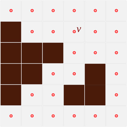
FIGURE 1. Discrete representation of the planar configuration space, C. The dark brown cells are inaccessible (obstacles), and a vertex corresponds to each accessible cell.
1.3 Contributions
The main contributions of this paper are novel methods for pursuer-to-evader assignment in presence of uncertainties for total capture time minimization as well as for maximum capture time minimization. We also present a novel control algorithm for pursuers based on Theta* search (Nash et al., 2007) that takes the evaders’ probability distribution into account, and present a control strategy for evaders that try to actively avoid the pursuers trying to capture it. We assume that both groups of agents (pursuers and evaders) are aware of the control strategies employed by the other group, and can use that knowledge to predict and update the probability distributions that are used for internal representations of the competing group.
1.4 Overview of the Paper
Section 3 provides the technical tools and background for formally describing the problem. In Section 4, we introduce the control strategies for the evaders and pursuers. In presence of uncertainties this control strategy becomes a stochastic one. We also describe how each type of agent predict and update the probability distributions representing the other type using this known control strategy. In Section 5, we present algorithms for assigning pursuers to the probabilistic evaders so as to minimize the expected time to capture. In Section 6 simulation and comparison results are presented.
2 Related Work
The pursuit-evasion problem in a probabilistic setting requires localization of the evaders as well as development of a controller for the pursuer to enable it to capture the evader. Markov localization is an effective approach for tracking probabilistic agents in unstructured environments since it is capable of representing probability distributions more general than normal distributions [unlike Kalman filters (Barshan and Durrant-Whyte, 1995)]. Compared to Monte Carlo or particle filters (Fox et al., 1999a; Fox et al., 1999b), Markov localization is often computationally less intensive, more accurate and has stronger formal underpinnings.
Markov localization has been widely used for estimating an agent’s position in known environments (Burgard et al., 1996) and in dynamic environments (Fox et al., 1999b) using on-board sensors, as well as for localization of evaders using noisy external sensors (Fox et al., 1998; Fox et al., 1999b; Zhang, 2007a). More recently, in conjunction with sensor fusion techniques, Markov localization has been used for target tracking using multiple sensors (Zhang, 2007b; Nagaty et al., 2015).
Detection and pursuit of an uncertain or unpredictable evader has also been studied extensively. (Chung et al., 2011) provides a taxonomy of search and pursuit problems in mobile robotics. Different methods are compared in both graphs and polygonal environments. Under that taxonomy, our work falls under the domain of probabilistic search problems with multiple heterogeneous searchers/pursuers and multiple targets on a finite graph representation of the environment. Importantly, this survey however notes that the minimization of distance and time to capture the evaders is less studied. (Khan et al., 2016) is another comprehensive review focused on cooperative multi-robot targets observation. (Hollinger et al., 2007) describes strategies for pursuit-evasion in an indoor environment which is discretized into different cells, with each cell representing a room. However, in our approach, the environment is discretized into finer grids that generalize to a wider variety of environments. In (Hespanha et al., 1999) a probabilistic framework for a pursuit-evasion game with one evader and multiple pursuers is described. A game-theoretic approach is used in (Hespanha et al., 2000) to describe a pursuit-evasion game in which evaders try to actively avoid the pursuers. (Makkapati and Tsiotras, 2019) describes an optimal strategy for evaders in multi-agent pursuit-evasion without uncertainties. Along similar lines, in (Oyler et al., 2016) the authors describe a pursuit-evasion game in presence of obstacles in the environment. (Shkurti et al., 2018) describes a problem involving a robot that tries to follow a moving target using visual data. Patrolling is another approach to pursuit-evasion problems in which persistent surveillance is desired. Multi-robot patrolling with uncertainty have been studied extensively in (Agmon et al., 2009), (Agmon et al., 2012) and (Talmor and Agmon, 2017). More recently in (Shah and Schwager, 2019), Voronoi partitioning has been used to guide pursuers to maximally reduce the area of workspace reachable by a single evader. Voronoi partitioning along with area minimization has also been used for pursuer-to-evader assignments in problems involving multiple deterministic and localized evaders and pursuers (Pierson et al., 2017).
3 Problem Formulation
3.1 Representing the Pursuers, Evaders, and Environment
Since the evaders are represented by probability distributions by the pursuers, the time-to-capture an evader by a particular pursuer is a stochastic variable. We thus consider the problems of pursuer-to-evader assignment and computation of control velocities for the pursuers with a view of minimizing the total expected capture time (the sum of the times taken to capture each of the evaders) or the maximum expected capture time (the maximum out of the times taken to capture each of the evaders). We assume that the number of pursuers is greater that the number of evaders and that the pursuers constitute a heterogeneous team, with each having different maximum speeds and different capture capabilities. The speed of the pursuers are assumed to be higher than the evaders to enable capture in any environment (even obstacle-free or unbounded environment). The objective of this paper is to design strategies for the pursuers to assign themselves to the evaders, and in particular, algorithms for assignment of the excess (redundant) pursuers, so as to minimize the total/maximum expected capture time.
While the evaders know the pursuers’ assignment strategy, they don’t know the pursuers’ positions, the probability distributions that the pursuers use to represent the evaders, or the exact assignment that the evaders determine. Instead, the evaders rely on the probability distributions that they use to represent the pursuers to figure out the assignments that the pursuers are likely using. We use a Markov localization (Thrun et al., 2005) technique to update the probability distribution of each agent.
Throughout this paper we use the following notations to represent the agents and the environment:
Configuration Space Representation: We consider a subset of the Euclidean plane,
Agents: The ith pursuer’s location is represented by ri ∈ V, and the jth evader by yj ∈ V (we will use the same notations to refer to the respective agents themselves). The set of the indices of all the pursuers is denoted by
Heterogeneity: Pursuer ri is assumed to have a maximum speed of vi, and the objective being time minimization, it always maintains that highest possible speed. It also has a capture radius (i.e., the radius of the disk within which it can capture an evader) of ρi.
3.2 Probabilistic Representations
The pursuers represent the jth evader by a probability distribution over V denoted by
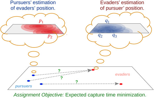
FIGURE 2. Problem overview.
3.2.1 Motion Model
At every time-step the known control strategy (hence, known transition probabilities) allows one type of agent to predict the probability distribution of the other type of agent in the next time-step:
where using the first equation the pursuers predict the jth evader’s probability distribution at the next time-step using the transition probabilities Kj computed using the known control strategy of the evader. While the second equation is used by the evaders to predict the ith pursuer’s probability distribution using transition probabilities Li computed from the known control strategy of the pursuers. These control strategies and the resulting transition probabilities will be discussed in more details in Sections 4.1 and 4.2.
3.2.2 Sensor Model
We assume that the probability that a pursuer at r ∈ V measures signal s (in some discrete signal space
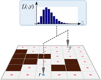
FIGURE 3. For fixed r, y, the plot shows the probability distribution over the signal space
Using Bayes’ rule, the updated probability distribution of the jth evader as computed by a pursuer at, r, based on sensor measurement, st, and the prior probability estimate,
If multiple signals,
Likewise, the evaders y1, y2, ⋯ measuring signals
The specific functional form for f and h depend not only on the distance between the pursuers and the evaders in the environment, but also on the obstacles that results on degradation of the signals emitted by the agents. The details of the specific sensor models appear in the “Results” section (Section 6).
3.3 Assignment Fundamentals
The goal for our assignment strategy is to try to find the assignment that minimizes either the total expected capture time (the sum of the times taken to capture each of the evaders in
3.3.1 Formal Description of Assignment
In order to formally describe the assignment problem, we use the following notations:
Assignment: The set of pursuers assigned to the jth evader will be represented by the set Ij. The individual assignment of ith pursuer to jth evader will be denoted by the pair (i, j).
A (valid) assignment,
The set of all possible valid assignments is denoted by
3.3.2 Probabilistic Assignment Costs
In this section we consider the time that pursuer i takes to capture evader j. We describe the computation from the perspective of the pursuers. Since the evader j is represented by the probability distribution, pj, over V, we denote Tij as the random variable representing the uncertain travel time from pursuer i to evader j. The probability that Tij falls within a certain interval is the sum of all the probabilities on the vertices of V such that the travel time from ri to the vertex is within that interval. That is,
We first note that Tij and Tij′ are independent variables whenever j and j′ are different (i.e., the time taken to reach evader j does not depend on time taken to reach evader j′). However, Tij and Ti′j are dependent random variables since, for a given travel time (and hence travel distance) from pursuer i to evader j, and knowing the distance between pursuers i and i′, the possible values of distances between pursuer i′ and evader j are constrained by the triangle inequality. That is, for any given j, the random variables in the set
Thus, in order to compute the joint probability distributions of
3.4 Problem Objectives
In the next sections we will describe the control strategy used by a pursuer that allows it to effectively capture the evader assigned to it, as well as the control strategy of an evader that allows it to move away from the pursuers assigned to it.
In Section 5, for designing the assignment strategy for the pursuers we will consider two metrics to minimize: 1) the total expected capture time, which is the sum of the times taken to capture each of the evaders, and, 2) the maximum expected capture time, which is the times taken to capture the last evader. While the actual assignment is computed by the pursuers and unavailable to the evaders, the evaders will estimate the likely assignment in order to determine their control strategy.
As mentioned earlier, we assume that both types of agents know all the strategies used by the other type of agents. That is, the pursuers know the evaders’ control strategy and the evaders know the pursuers’ control and assignment strategies. However the pursuers do not know the evaders’ exact position and vice versa. Instead they reason about that by maintaining probability distributions representing the positions of the other type of agents and update those distributions using the known control strategies of the other type of agents and weak signals measured by onboard sensors.
4 Control Strategies
Assuming a known pursuer-to-evader assignment, in this section we describe the control strategies used by the evaders to avoid being captured and the control strategy used by the pursuers to capture the evaders.
4.1 Evader Control Strategy
In presence of pursuers, an evader yj actively tries to move away from the pursuers targeting it. With the evader at y ∈ V and deterministic pursuers,
where
In order to determine the best action that the evader at y′ ∈ V can take, it computes the marginal increase in τ if it moves to y ∈ V (Figure 4):
where ϵ is a small number that gives a small positive marginal increase for some neighboring vertices in scenarios when the evader gets cornered against an obstacle.
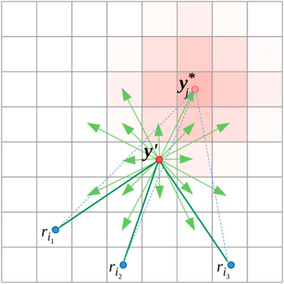
FIGURE 4. Illustration of control strategy of evader at y′. Transition probabilities, Kj (⋅, y′) are shown in light red shade.
4.1.1 Evader’s Control Strategy
In a deterministic setup the evader at y′ will move to
where Ay′ refers to the states/vertices in the vicinity of y′ that the evader can transition to in the next time-step. But, in the probabilistic setup where the evaders represent the ith pursuer by the distribution qi, with every y ∈ Ay′ an evader associates a probability that it is indeed the best transition to make. In practice, these probabilities are computed by sampling
4.1.2 Pursuer’s Prediction of Evader’s Distribution Based on Known Evader Control Strategy
The pursuers know the evader’s strategy of maximizing the marginal increase in capture time. However, they do not know the evaders’ exact position, nor do they know the distributions, qi, that the evaders maintain of the pursuers. The uncertainty in the action of the evader due to that is modeled by a normal distribution centered at
where, for simplicity, df is assumed to be the Euclidean distance between the neighboring vertices in the graph, and κj is a normalization factor so that ∑y∈VK(y, y′) = 1.
4.2 Pursuer Control Strategy
A pursuer, ri ∈ Ij, pursuing the evader at yj needs to compute a velocity for doing so.
In a deterministic setup, if the evader is at yj ∈ V, the pursuer’s control strategy is to follow the shortest (geodesic) path in the environment connecting ri to yj. This controller, in practice, can be implemented as a gradient-descent of the square of the path metric (geodesic distance) and is given by
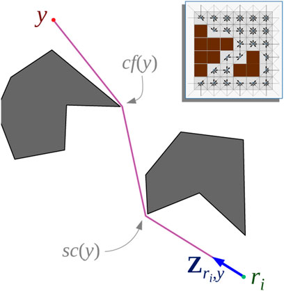
FIGURE 5. Theta* algorithm is used on a 8-connected grid graph, G✳ (top right inset) for computing geodesic distances as well as control velocities for the pursuers.
4.2.1 Pursuer’s Control Strategy
Since the pursuers describe the jth evader’s position by the probability distribution
Since the pursuer has a maximum speed of vi, and the exact location of the evader is unknown, we always choose the maximum as speed for the pursuer:
For computing dg (ri, y) we use the Theta* search algorithm (Nash et al., 2007) on a uniform 8-connected square grid graph, G✳, representation of the environment (Figure 5 inset). While very similar to Dijkstra’s and A*, Theta* computes paths that are not necessary restricted to the graph and are closer to the true shortest path in the environment. While more advanced variations of the algorithm exists [such as Lazy Theta* (Nash et al., 2010) and Incremental Phi* (Nash et al., 2009)], we choose to use the most basic variety for simplicity. Computation of the sum in Equation 9 can also be performed during the Theta* search. Algorithm 1 describes the computation of dg (ri, y) (the shortest path (geodesic) distance between ri and a point y in the environment) and the control velocity vi.
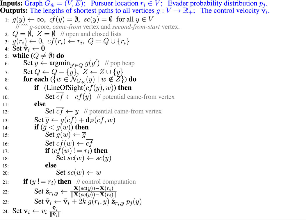
Algorithm 1. Theta* Based Pursuer Control
The algorithm is reminiscent of Dijkstra’s search, maintaining an open list, Q, and expanding the least g-score vertex at every iteration, except that the came-from vertex (cf) of a vertex can be a distant predecessor determined by line of sight (Lines 10–14) and the summation in (9) is computed on-the-fly during the execution of the search (Line 28).
We start the algorithm by initiating the open list with the single start vertex, ri, set its g-score to zero, and its came-from vertex, c f, to reference to itself (line 4). Every time a vertex, y (one with the minimum g-score in the open list, maintained using a heap data structure), is expanded, Theta* checks for the possibility of updating a neighbor, w, from the set of neighbors,
4.2.2 Evader’s Prediction of Pursuer’s Distribution Based on Known Pursuer Control Strategy
Since the evaders represent the ith pursuer using the probability distribution qi, they need to predict the pursuer’s probability distribution in the next time step knowing the pursuer’s control strategy. This task is assigned to the jth evader such that i ∈ Ij (we define
where κi is the normalization factor.
5 Assignment Strategies
We first consider the assignment problem from the perspective of the pursuers—with the evaders represented by probability distributions
5.1 Expected Capture Time Minimization for an Initial One-To-One Assignment
In order to determine an initial assignment
Since for every
Thus, for computing the initial assignment, it is sufficient to use the numerical costs of
5.1.1 Modified Hungarian Algorithm for Minimization of Maximum Capture Time
For finding the initial assignment that minimizes the maximum expected capture time, we develop a modified version of the Hungarian algorithm. To that end we observe that in a Hungarian algorithm, instead of using the expected capture times as the costs, we can use the p-th powers of the expected capture times,
In a simple implementation of the Hungarian algorithm (Munkres, 1957), one performs multiple row and column operations on the cost matrix wherein a specific element of the cost matrix, Ci′j′, is added or subtracted from all the elements of a selected subset of rows and columns. Thus, if we want to use the pth powers of the costs, but choose to maintain only the costs in the matrix (without explicitly raising them to the power of p during storage), for the row/column operations we can simply raise the elements of the matrix to the power of p right before the addition/subtraction operations, and then take the pth roots of the results before updating the matrix entries. That is, addition of Ci′j′ to an element Cij will be replaced by the operation
Thus, letting p → ∞, we have Cij ⊕∞Ci′j′ = max{Cij, Ci′j′} and
5.2 Redundant Pursuer Assignment Approach
After computation of an initial assignment,
Notably, the work in (Prorok, 2020) shows that a cost function such as (12), which considers redundant assignment under uncertain travel time, is supermodular. It follows that the assignment procedure can be implemented with a greedy algorithm that selects redundant pursuers near-optimally3.
Algorithm 2 summarizes our greedy redundant assignment algorithm. At the beginning of the algorithm, we sample h
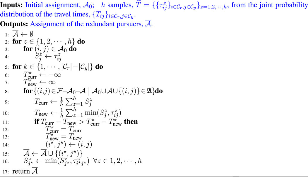
Algorithm 2. Total Time minimization Redundant Pursuer Assignment
In this algorithm, we first consider the initial assignment,
In Line 10, we loop over all the possible pursuer-to-evader pairings, (i, j), that are not already present in
5.3 Equality in Marginal Gain
One way that the inequality condition in Line 13 gets violated is when the marginal gains Tcurr − Tnew and
In order to address this issue properly, we maintain a list of “potential assignments” that corresponds to (i, j) pairs (along with the corresponding Tnew values maintained as an associative list,
5.3.1 Redundant Pursuer Assignment for Minimization of Maximum Capture Time
As for the minimization of the maximum expected capture time in the redundant assignment process, we take a similar approach as in Section 5.1.1. We first note that choosing
Thus assigning a redundant pursuer to an evader (out of the assignments that produce the same marginal gain) that has the maximum expected capture time, thus providing some extra help with catching the pursuer.
With these modifications, an assignment for the redundant pursuers can be found that minimizes the maximum expected capture time instead of total expected capture time. We call this redundant pursuer assignment algorithm “Maximum Time minimization Redundant Pursuer Assignment” (MTRPA).
5.4 Evader’s Estimation of Pursuer Assignment
Knowing the assignment strategy used by the pursuers, but the pursuers represented by the probability distributions
6 Results
For the sensor models, f, h, we emulate sensing electromagnetic radiation in the infrared or radio spectrum emitted by the evaders/pursuers. Wi-fi signals and thermal signatures are such examples. For simplicity, we ignore reflection of the radiation from surfaces, and only consider a simplified model for transmitted radiation. If Ir,y is the line segment connecting the source, y, of the radiation to the location of a sensor, r, and is parameterized by segment length, l, we define effective signal distance,
The motion models for predicting the probability distributions are chosen as described in Section 4.1.2 and 4.2.2.
For the parameter we choose ϵ(y) ∈ (0, 0.3) (in Equation 6) depending on whether or not y is close to an obstacle. The pursuer (resp. evader) choose σj = 0.3 (resp. σi = 0.3) for modeling the uncertainties in the evaders’ (resp. pursuers’) estimate of the pursers’ (resp. evaders’) positions.
We Compared the Performance of the Following Algorithms
• Total Time minimizing Pursuer Assignment (TTPA): This assignment algorithm uses the basic Hungarian algorithm for computing the initial assignment
• Maximum Time minimizing Pursuer Assignment (MTPA): This assignment algorithm uses the modified Hungarian algorithm described in Section 5.1.1 for computing the initial assignment
• Nearest Neighbor Assignment (NNA): In this algorithm we first construct a
We evaluated the algorithms in two different environments: Game maps “AR0414SR” and “AR0701SR” from 2D Pathfinding Benchmarks (Sturtevant, 2012) see Figure 6. For different pursuer-to-evader ratios in these environments, we ran 100 simulations each. For each simulation, in environment “AR0414SR”, the initial positions of pursuers and evaders were randomly generated, while in environment :“AR0701SR” the initial position of the pursuers were randomly generated in the small central circular region and the initial position of the evaders were randomly generated in the rest of the environment. For each generated initial conditions we ran the three algorithms, TTPA, MTPA and NNA, to compare their performance.
1) Max capture time in “AR0414SR”
2) Max capture time in “AR0701SR”
3) Total capture time in “AR0414SR”
4) Total capture time in “AR0701SR”
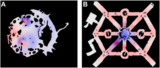
FIGURE 6. Environments for which statistic are presented. (A) “AR0414SR”; (B) “AR0701SR.” Each Panel also shows an example of the agent positions and distributions during one of the simulations. Blue hue indicates the evaders’ prediction of pursuers’ distributions,
Figure 7 shows a comparison between the proposed pursuer assignment algorithms (TTPA and MTPA) and the NNA algorithm for the aforementioned environments. From the comparison it is clear that the MTPA algorithm consistently outperforms the other algorithms with respect to the maximum capture time (Figure 7A), while TTPA consistently outperforms the other algorithms with respect to the total capture time (Figure 7C). In addition, Table 1 shows win rates of TTPA and MTPA over NNA (for TTPA this is the proportion of simulations in which the total capture time for TTPA was lower than NNA, while for MTPA this is the proportion of simulations in which the total capture time for MTPA was lower than NNA). TTPA has a win rate of around 60%, and MTPA has a win rate of over 70%.
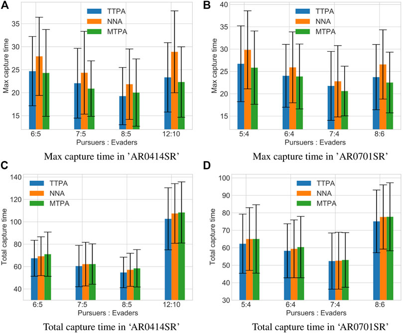
FIGURE 7. Comparison of the average values of maximum capture times (A, B) and total capture times (C, D) along with the standard deviation in different environments and with different pursuer-to-evader ratios using the TTPA, NNA and MTPA algorithms. Each bar represents data from 100 simulations with randomized initial conditions.

TABLE 1. Win rates of TTPA and MTPA algorithms over NNA. For a given set of initial conditions (initial position of pursuers and evaders), if TTPA takes less total time to capture all the evaders than NNA, it is considered a win for TTPA. While if MTPA takes less time to capture the last evader (maximum capture time) than NNA, it is considered as a win for MTPA.
Clearly the advantage of the proposed greedy supermodular strategy for redundant pursuer assignment is statistically significant. Unsurprisingly, we also observe that.increasing the number of pursuers tends to decrease the capture time.
1) Max capture time in “AR0414SR” with 7 pursuers and 5 evaders.
2) Total capture time in “AR0414SR” with 7 pursuers and 5 evaders.
Figure 8 shows a comparison of the total and maximum capture times with varying measurement noise level (varying k2) in the environment “AR0414SR” with a fixed number of pursuers and evaders, and with 20 randomly generated initial conditions. As expected, higher noise leads to more capture time for all the algorithms. However MTPA still outperforms the other algorithms w.r.t. maximum capture time, while TTPA outperforms the other algorithms w.r.t. the total capture time.
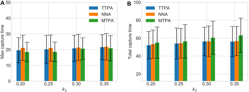
FIGURE 8. The effect of varying measurement noise level on maximum capture time (A) and total capture time (B).
7 Conclusion and Discussions
In this paper, we considered a pursuit-evasion problem with multiple pursuers, and multiple evaders under uncertainties. Each type of agent (pursuer or evader) represents the individuals of the other type using probability distributions that they update based on known control strategies and noisy sensor measurements. Markov localization is used to update a probability distributions. The evaders use a control strategy to actively evade the pursuers, while each pursuer use a control algorithm based on Theta* search for reducing the expected distance to the probability distribution of the evader that it’s pursuing. We used a novel redundant pursuer assignment algorithm which utilizes an excess number of pursuers to minimize the total or maximum expected time to capture the evaders. Our simulation results have shown a consistent and statistically significant reduction of time to capture when compared against a nearest-neighbor algorithm.
We considered a very complex problem setup that is not only stochastic in nature (each type of agent representing the other type of agents using probability distributions that are updated using a Markov localization model on a graph), but the environment is non-convex (due to presence of obstacles). While a general stability or convergence guarantee is extremely difficult, if not impossible, in such a complex problem setup, we can consider a simplified scenario for observing some of the stability and convergence properties of the control algorithm used by the pursuers. Such a simplified analysis has been provided in the Appendix below.
Data Availability Statement
The raw data supporting the conclusions of this article will be made available by the authors, without undue reservation.
Author Contributions
LZ was responsible for implementing the algorithms described in the paper, running simulations, generating numerical results as well as drafting majority of the results section. AP was responsible for developing the redundant pursuer assignment algorithm, overseeing its integration with the multi-agent control algorithms, and drafting the section on redundant pursuer assignment algorithm. SB was responsible for the development of pursuer and evader control algorithms, probabilistic representation and estimation algorithms, algorithms for initial pursuer-to-evader assignment, drafting of the corresponding technical sections in the paper, and overseeing the implementation and integration of all the different algorithmic components of the paper. All three authors contributed equally to the final writing and integration of the different sections of the paper, including the introductory and the conclusion sections.
Conflict of Interest
The authors declare that the research was conducted in the absence of any commercial or financial relationships that could be construed as a potential conflict of interest.
Publisher’s Note
All claims expressed in this article are solely those of the authors and do not necessarily represent those of their affiliated organizations, or those of the publisher, the editors and the reviewers. Any product that may be evaluated in this article, or claim that may be made by its manufacturer, is not guaranteed or endorsed by the publisher.
Footnotes
1Some parts of this paper appeared as an extended abstract in the proceeding of the 2019 IEEE International Symposium on Multi-robot and Multi-agent Systems (MRS) (Zhang et al., 2019).
2The expectation of the sum of two or more independent random variables is the sum of the expectations of the variables
3We note that without an initial assignment
References
Agmon, N., Fok, C.-L., Emaliah, Y., Stone, P., Julien, C., and Vishwanath, S. (2012). “On Coordination in Practical Multi-Robot Patrol,” in 2012 IEEE International Conference on Robotics and Automation, Saint Paul, MN, May 14–18, 2012, 650–656. doi:10.1109/ICRA.2012.6224708
Agmon, N., Kraus, S., Kaminka, G. A., and Sadov, V. (2009). “Adversarial Uncertainty in Multi-Robot Patrol,” in Twenty-First International Joint Conference on Artificial Intelligence, Pasadena, CA, July 11–17, 2009.
Barshan, B., and Durrant-Whyte, H. F. (1995). Inertial Navigation Systems for mobile Robots. IEEE Trans. Robot. Automat. 11, 328–342. doi:10.1109/70.388775
Bhattacharya, S., Ghrist, R., and Kumar, V. (2014). Multi-robot Coverage and Exploration on Riemannian Manifolds with Boundaries. Int. J. Robotics Res. 33, 113–137. doi:10.1177/0278364913507324
Burgard, W., Fox, D., Hennig, D., and Schmidt, T. (1996). “Estimating the Absolute Position of a mobile Robot Using Position Probability Grids,” in Proceedings of the Thirteenth National Conference on Artificial Intelligence - Volume 2, Portland, OR, August 4, 1996 (Palo Alto, CA: AAAI Press), 896–901. AAAI’96.
Chung, T. H., Hollinger, G. A., and Isler, V. (2011). Search and Pursuit-Evasion in mobile Robotics. Auton. Robot 31, 299–316. doi:10.1007/s10514-011-9241-4
Cortes, J., Martinez, S., Karatas, T., and Bullo, F. (2004). Coverage Control for mobile Sensing Networks. IEEE Trans. Robot. Automat. 20, 243–255. doi:10.1109/tra.2004.824698
Fox, D., Burgard, W., Dellaert, F., and Thrun, S. (1999a). “Monte Carlo Localization: Efficient Position Estimation for mobile Robots,” in Proceedings of the National Conference on Artificial Intelligence (Palo Alto, CA: AAAI), 343–349.
Fox, D., Burgard, W., and Thrun, S. (1998). Active Markov Localization for mobile Robots. Robotics Autonomous Syst. 25, 195–207. doi:10.1016/s0921-8890(98)00049-9
Fox, D., Burgard, W., and Thrun, S. (1999b). Markov Localization for mobile Robots in Dynamic Environments. jair 11, 391–427. doi:10.1613/jair.616
Hespanha, J. P., Kim, H. J., and Sastry, S. (1999). “Multiple-agent Probabilistic Pursuit-Evasion Games,” in Decision and Control, 1999. Proceedings of the 38th IEEE Conference on, Phoenix, AZ, December 7–10, 1999 (IEEE) 3, 2432–2437.
Hespanha, J. P., Prandini, M., and Sastry, S. (2000). “Probabilistic Pursuit-Evasion Games: A One-step Nash Approach,” in Decision and Control, 2000. Proceedings of the 39th IEEE Conference on, Sydney, Australia, December 12–15, 2000 (IEEE) 3, 2272–2277.
Hollinger, G., Kehagias, A., and Singh, S. (2007). “Probabilistic Strategies for Pursuit in Cluttered Environments with Multiple Robots,” in Robotics and Automation, 2007 IEEE International Conference on, Rome, Italy, April 10–14, 2007 (IEEE), 3870–3876. doi:10.1109/robot.2007.364072
Khan, A., Rinner, B., and Cavallaro, A. (2016). Cooperative Robots to Observe Moving Targets: Review. IEEE Trans. Cybernetics 48, 187–198. doi:10.1109/TCYB.2016.2628161
Makkapati, V. R., and Tsiotras, P. (2019). Optimal Evading Strategies and Task Allocation in Multi-Player Pursuit-Evasion Problems. Dyn. Games Appl. 9, 1168–1187. doi:10.1007/s13235-019-0031910.1007/s13235-019-00319-x
Munkres, J. (1957). Algorithms for the Assignment and Transportation Problems. J. Soc. Ind. Appl. Math. 5, 32–38. doi:10.1137/0105003
Nagaty, A., Thibault, C., Trentini, M., and Li, H. (2015). Probabilistic Cooperative Target Localization. IEEE Trans. Automat. Sci. Eng. 12, 786–794. doi:10.1109/TASE.2015.2424865
Nash, A., Daniel, K., Koenig, S., and Felner, A. (2007). “Theta*: Any-Angle Path Planning on Grids,” in AAAI (Palo Alto, CA: AAAI Press), 1177–1183.
Nash, A., Koenig, S., and Likhachev, M. (2009). “Incremental Phi*: Incremental Any-Angle Path Planning on Grids,” in International Joint Conference on Artificial Intelligence (IJCAI), Pasadena, CA, July 11–17, 2009, 1824–1830.
Nash, A., Koenig, S., and Tovey, C. (2010). “Lazy Theta*: Any-Angle Path Planning and Path Length Analysis in 3d,” in Proceedings of the AAAI Conference on Artificial Intelligence, Atlanta, Georgia, July 11–15, 2010. 24.
Oyler, D. W., Kabamba, P. T., and Girard, A. R. (2016). Pursuit-evasion Games in the Presence of Obstacles. Automatica 65, 1–11. doi:10.1016/j.automatica.2015.11.018
Pierson, A., Wang, Z., and Schwager, M. (2017). Intercepting Rogue Robots: An Algorithm for Capturing Multiple Evaders with Multiple Pursuers. IEEE Robot. Autom. Lett. 2, 530–537. doi:10.1109/LRA.2016.2645516
Prorok, A. (2020). Robust Assignment Using Redundant Robots on Transport Networks with Uncertain Travel Time. IEEE Trans. Automation Sci. Eng. 17, 2025–2037. doi:10.1109/tase.2020.2986641
Rimon, E., and Koditschek, D. E. (1992). Exact Robot Navigation Using Artificial Potential Functions. IEEE Trans. Robot. Automat. 8, 501–518. doi:10.1109/70.163777
Shah, K., and Schwager, M. (2019). “Multi-agent Cooperative Pursuit-Evasion Strategies under Uncertainty,” in Distributed Autonomous Robotic Systems (Springer), 451–468. doi:10.1007/978-3-030-05816-6_32
Shkurti, F., Kakodkar, N., and Dudek, G. (2018). “Model-based Probabilistic Pursuit via Inverse Reinforcement Learning,” in 2018 IEEE International Conference on Robotics and Automation (ICRA), Brisbane, Australia, May 21–25, 2018 (IEEE), 7804–7811. doi:10.1109/icra.2018.8463196
Sturtevant, N. R. (2012). Benchmarks for Grid-Based Pathfinding. IEEE Trans. Comput. Intell. AI Games 4, 144–148. doi:10.1109/tciaig.2012.2197681
Talmor, N., and Agmon, N. (2017). “On the Power and Limitations of Deception in Multi-Robot Adversarial Patrolling,” in Proceedings of the Twenty-Sixth International Joint Conference on Artificial Intelligence, IJCAI-17, Melbourne, Australia, August 19, 2017, 430–436. doi:10.24963/ijcai.2017/61
Thrun, S., Burgard, W., and Fox, D. (2005). Probabilistic Robotics (Intelligent Robotics and Autonomous Agents). The MIT Press.
Zhang, L., Prorok, A., and Bhattacharya, S. (2019). “Multi-agent Pursuit-Evasion under Uncertainties with Redundant Robot Assignments: Extended Abstract,” in IEEE International Symposium on Multi-Robot and Multi-Agent Systems, New Brunswick, NJ, August 22–23, 2019. Extended Abstract. doi:10.1109/mrs.2019.8901055
Zhang, W. (2007a). A Probabilistic Approach to Tracking Moving Targets with Distributed Sensors. IEEE Trans. Syst. Man. Cybern. A. 37, 721–731. doi:10.1109/tsmca.2007.902658
Zhang, W. (2007b). A Probabilistic Approach to Tracking Moving Targets with Distributed Sensors. IEEE Trans. Syst. Man. Cybern. A. 37, 721–731. doi:10.1109/TSMCA.2007.902658
Appendix: Simplified Theoretical Analysis
Suppose evader j is assigned to pursuer i and this assignment does not change. We consider the case when the evader’s maximum speed is negligible compared to the pursuer’s speed, as a consequence of which we make the simplifying assumption that the evader is stationary. The first observation that we can make is that with the stationary evader, the probability distribution for the evader’s pose is updated according to
Hence, after a sufficiently long period of time the evader is fully localized. The control law in (9), by construction, simply becomes following the negative of the gradient of the square of the geodesic distance to the evader (see first paragraph of Section 4.2). This ensures that the geodesic distance to the evader is decreased at every time-step (formally, the geodesic distance can be considered as a Lyapunov functional candidate the time derivative of which is always negative and zero when the pursuer and the evader are at the same location), hence ensuring the eventual capture of the evader. We summarize this simplified analysis under the following proposition:
Proposition (informal): For a fixed persuer-to-evader assignment, if the evader’s maximum speed is negligible compared to the pursuer’s speed, and if the sensing model for the sensor onboard the pursuer is unbiased, after a sufficiently long period of time the control law in (9) will make the pursuer’s position asymptotically converge to the position of the evader.
Keywords: multi-robot systems, pursuit-evasion, probabilistic robotics, redundant robots, assignment
Citation: Zhang L, Prorok A and Bhattacharya S (2021) Pursuer Assignment and Control Strategies in Multi-Agent Pursuit-Evasion Under Uncertainties. Front. Robot. AI 8:691637. doi: 10.3389/frobt.2021.691637
Received: 06 April 2021; Accepted: 31 July 2021;
Published: 17 August 2021.
Edited by:
Savvas Loizou, Cyprus University of Technology, CyprusReviewed by:
Nicholas Stiffler, University of South Carolina, United StatesNing Wang, Harbin Engineering University, China
Copyright © 2021 Zhang, Prorok and Bhattacharya. This is an open-access article distributed under the terms of the Creative Commons Attribution License (CC BY). The use, distribution or reproduction in other forums is permitted, provided the original author(s) and the copyright owner(s) are credited and that the original publication in this journal is cited, in accordance with accepted academic practice. No use, distribution or reproduction is permitted which does not comply with these terms.
*Correspondence: Subhrajit Bhattacharya, c3ViMjE2QGxlaGlnaC5lZHU=