 Mengxue Hou
 Sungjin Cho
 Haomin Zhou
 Catherine R. Edwards
 Fumin Zhang
- 1Electrical and Computer Engineering, Georgia Institute of Technology, Atlanta, GA, United States
- 2Department of Guidance and Control, Agency for Defense Development, Daejeon, South Korea
- 3School of Mathematics, Georgia Institute of Technology, Atlanta, GA, United States
- 4Skidaway Institute of Oceanography, University of Georgia, Savannah, GA, United States
A bounded cost path planning method is developed for underwater vehicles assisted by a data-driven flow modeling method. The modeled flow field is partitioned as a set of cells of piece-wise constant flow speed. A flow partition algorithm and a parameter estimation algorithm are proposed to learn the flow field structure and parameters with justified convergence. A bounded cost path planning algorithm is developed taking advantage of the partitioned flow model. An extended potential search method is proposed to determine the sequence of partitions that the optimal path crosses. The optimal path within each partition is then determined by solving a constrained optimization problem. Theoretical justification is provided for the proposed extended potential search method generating the optimal solution. The path planned has the highest probability to satisfy the bounded cost constraint. The performance of the algorithms is demonstrated with experimental and simulation results, which show that the proposed method is more computationally efficient than some of the existing methods.
1 Introduction
Over the last few decades, autonomous underwater vehicles (AUVs) have been employed for ocean sampling (Leonard et al., 2010; Smith et al., 2010), surveillance and inspection (Ozog et al., 2016; Xiang et al., 2010), and many other applications. Ocean flow is the dominant factor that affects the motion of AUVs (Zhang et al., 2016). Ocean flow dynamics vary in both space and time, and can be represented as geophysical Partial Differential Equations (PDEs) in ocean circulation models (e.g., the Regional Ocean Modeling System (ROMS, Shchepetkin and McWilliams, 2005; Haidvogel et al., 2008) and the Hybrid Coordinate Ocean Model (HYCOM, Chassignet et al., 2007)). While these models can provide flow information over a large spatial domain and forecast over several days, the available flow field forecast may still contain high uncertainty and error. The uncertainty comes from multiple sources, including the incomplete physics or boundary conditions (Haza et al., 2007; Griffa et al., 2004) and even terms in the equations themselves (Lermusiaux, 2006). In addition, the high complexity of the flow dynamics makes solving these PDEs computationally expensive. Data-driven flow models (Mokhasi et al., 2009; Chang et al., 2014) can provide short-term flow prediction in a relatively smaller area with significantly lower computational cost, and can be more suitable for supporting real-time AUV navigation, particularly for systems with strong gradients and/or high uncertainty.
Path planning is one of the crucial and fundamental functions to achieve autonomy. Two key considerations for an AUV path planner are computational efficiency and path quality. The path planning strategy should be computationally efficient so that the time for generating a path can be kept to a minimum. When these methods are sufficiently fast, path planning can be performed in near-real time, generating a feasible solution in minutes while the AUV has surfaced to get a GPS fix and communicate with shore. Advantages of real time path planning are that more recent information, including the real time data from the vehicle, can be incorporated in path planning. Hence there will be less planning error due to outdated information (Leonard et al., 2010). At the same time, it is desired that the path planning algorithm has theoretical guarantee on the quality of the generated path.
Most path planning algorithms aim to design optimal path minimizing certain cost, for example, those associated with engineering or flight characteristics (battery life, travel time) or scientific value (e.g., distance relative to other assets or spacing of relevant processes). Algorithms that have been applied to AUV optimal path planning include: 1) graph-based methods such as the A* method (Rhoads et al., 2012; Pereira et al., 2013; Kularatne et al., 2017, 2018) and the Sliding Wavefront Expansion (SWE) (Soulignac, 2011); 2) sampling-based methods like the Rapidly exploring Random Trees (RRTs) (Kuffner and LaValle, 2000; Cui et al., 2015), RRT* (Karaman and Frazzoli, 2011) and informed RRT* (Gammell et al., 2018); 3) methods that approximate the solution of HJ (Hamilton-Jacobi) equations, such as the Level Set Method (LSM) (Subramani and Lermusiaux, 2016; Lolla et al., 2014), and 4) the evolutionary algorithms, including the particle swarm optimization methods (Roberge et al., 2012; Zeng et al., 2014), and the differential evolution methods (Zamuda and Sosa, 2014; Zamuda et al., 2016). See (Zamuda and Sosa, 2019; Zeng et al., 2015; Panda et al., 2020) for a comprehensive review on the existing AUV path planning methods. However, the computational cost of the above mentioned methods could be high, especially in cases where the AUV deployment domain is large.
Using a regular grid to discretize the flow field can result in unnecessary large number of cells, which increases the computational burden of the graph search methods. Since the flow speed in adjacent cells is usually similar, we partition the flow field into piece-wise constant subfields, within each the flow speed is a constant vector, and introduce the Method of Evolving Junctions (MEJ) (Zhai et al., 2020) to solve the optimal path planning problem. MEJ solves for the optimal path by recasting the infinite dimensional path planning problem into a finite dimensional optimization problem through introducing a number of junction points, defined as the intersection between the path and the region boundaries. Hence the computation cost of MEJ is significantly lower than other optimal path planning methods, especially when the flow field is partitioned into a small number of cells (Zhai et al., 2020). We identify Soulignac. (2011) as the work closest related to ours, in which sliders, defined as points sliding on the partitioned region boundaries, are introduced to describe the wavefront expansion of the graph search methods. In each iteration of the wavefront expansion, each slider’s position on the wavefront is derived by minimizing the travel cost in a single cell, and then the planned path is computed by the backtracking of wavefronts. Both MEJ and SWE are based on a novel parameterization of the path by introducing the junctions and the sliders, that were discovered independently by the two research groups. The main difference between MEJ and SWE lies in that MEJ solves for junction positions by formulating a non-convex optimization problem, and derives the global minimizer by intermittent diffusion (Li et al., 2017), which intermittently adds white noise to the gradient flow, while SWE solves for slider positions by graph search methods. MEJ has been justified to find the global minimizer with probability 1. However, since the method does not pose any structure in the search, the computational cost of MEJ could be less favorable compared to SWE if the number of cells scales up.
To reduce the computational cost of the path planning problem, the search can be reduced to find paths with total cost less than an upper bound. Stern et al. (2014) present two algorithms to solve the bounded cost search problem: the Potential Search (PTS) and the Anytime Potential Search (APTS). The PTS method defines the Potential Ordering Function, which is an implicit evaluation of the probability that a node is on a path satisfying the bounded cost constraint, and iteratively expands the nodes in the graph with the highest Potential Ordering Function value. The wavefront expansion terminates when the goal node has been expanded, and the path is found by backtracking of the wavefronts. The APTS method runs the PTS algorithm iteratively to improve on the incumbent solution, with the upper bound on total cost lowered in each iteration of the algorithm. Later work (Thayer et al., 2012) improves on the PTS method by minimizing both the potential and an estimation of the remaining search effort, so that the bounded cost search problem will be solved faster.
In this paper, our first objective is to develop a data-driven computational flow model that approximates the true flow field in the region of interest to assist AUV path planning. The proposed data-driven flow model divides the flow field into cells, within which the flow is represented as a single flow vector. The optimal flow cell partition and initial values of the flow vectors in each cell are derived from prior flow information, from numerical ocean models or from observations. To improve model accuracy, AUV observational data can be incorporated into the data-driven model in near-real time, for example, in the form of observed or estimated velocities (Chang et al., 2015). Here, we design a learning algorithm that estimates the flow field parameters based on the AUV path data. Our second objective is to develop an algorithm that solves the AUV bounded cost path planning problem. Given that the vehicle is traveling in a flow field represented by the data-driven computational model, the goal is to design a path that connects AUV initial position with goal position with the highest probability to have travel cost less than a pre-assigned upper bound. By introducing the key function, which is an implicit evaluation function of the probability that a path satisfies the bounded cost constraint, the optimal path is computed by searching for the nodes with lowest key function value using an informed graph search method.
The main novelty of this work is introducing the modified PTS method to solve the bounded cost search problem. Unlike the PTS method (Stern et al., 2014), which assumes that the branch cost of the graph is known exactly, our method deals with problems where the branch cost of the graph is uncertain. Given assumptions on the distribution of cost-of-arrival and cost-to-go, we prove that the proposed algorithm guarantees optimality of the planned path, that is, the planned path has the highest probability of satisfying the bounded cost constraint. To the best of our knowledge, this is the first time that the optimality of the modified PTS solution to bounded cost problems is proved. The proposed bounded cost path planning method can be viewed as an extension to MEJ. Compared to MEJ, the modified PTS algorithm is computationally more efficient, since a graph search method is adopted to search for the junction positions. At the same time, optimality of the planned path can be theoretically justified. The major benefit of the proposed bounded cost path planning algorithm lies in that it plans a path faster, while at the same time still guarantees the path quality. This paper is a significant extension of the conference proceeding (Hou et al., 2019), which proposes a flow partition method that approximates the flow field by a set of cells of uniform flow speed. The main extensions of this paper are that taking advantage of the flow model proposed in (Hou et al., 2019), we propose the modified PTS method to solve the AUV bounded cost path planning problem, and present theoretical justification on the optimality of the proposed PTS method. The proposed bounded cost search method is potentially applicable for all bounded cost path planning problems with uncertain branch cost.
We believe the proposed data-driven flow modeling and bounded cost path planning methods are well-suited for path planning of underwater glider deployment near Cape Hatteras, NC, a highly dynamic region characterized by confluent western boundary currents and convergence in the adjacent shelf and slope waters. While deployed, the gliders are subject to rich and complex current fields driven by a combination and interaction of Gulf Stream, wind, and buoyancy forcing, with significant cross-shelf exchange on small spatial and temporal scales (Savidge et al., 2013a, Savidge et al., 2013b) that would be highly difficult to sample using traditional methods. Path planning must consider spatial variability of the flow field. Because spatial gradients are significant, real-time path planning is critical to take advantage of real-time data streams. Through simulated experiments, we demonstrate the performance of applying the proposed algorithms to underwater glider deployment in this area, and show that the proposed algorithm is more computationally efficient than A* and LSM.
2 Problem Formulation
2.1 Vehicle Dynamics
Let
where
Assumption 2.1: During the operation,
Remark 2.1: Actual vehicle speed may depend on a number of factors that affect an AUV’s speed, including water depth, efficiency of propulsion, and bio-fouling. These effects are difficult to estimate. Hence the vehicle forward speed is assumed to be an unknown constant.
Assumption 2.2: We assume that the heading
Remark 2.2: Though the actual location of a vehicle may only be known occasionally when the vehicle is underwater, the trajectory of the vehicle can be estimated through localization algorithms, which incorporates the known locations and the heading angle commands as inputs to generate the optimal state estimation.
Assumption 2.3: We assume the flow field is time-invariant throughout the deployment.
Remark 2.3: Even though there are existing work that considers the time-variant flow field in solving the AUV planning problem, such as (Eichhorn, 2013; Lolla et al., 2014; Zamuda and Sosa, 2014), we make this assumption due to the patterns of the flow field in this domain. In the domain of interest considered in this paper, which is near Cape Hatteras, NC, the current field is driven by a combination and interaction of Gulf Stream, wind, and buoyancy forcing (Savidge et al., 2013a, Savidge et al., 2013b). Because magnitude and spatial gradients of the flow field are significant relative to the temporal variation of the flow field (mostly the tidal flow component), time variation of the flow does not have a significant influence over the planned path.
2.2 Data-Driven Flow Modeling
Flow speed at neighboring grid points often exhibits similarity in both strength and direction. Hence we assume that at the time scale of an AUV deployment, the flow field can be divided into finite number of regions
This function indicates whether
In order to compute the partition, which is represented by the basis functions
After the optimal partition is computed from forecast or historical datasets, we need to compute the strength of the flow in each partition based on the path information of the AUV while moving through the flow field. Again, we assume that the true flow field is constant in each of the partitioned cell. Let
To estimate the true flow field
be our estimate of the parameter
2.3 Bounded Cost Path Planning
Our goal is to find a path connecting the vehicle current position
where the total travel time to start from the initial position
3 Flow Field Estimation
First let us describe Algorithm 1. We derive the spatial basis function and the initialized flow model parameters by solving eq. 2 using the K-means algorithm. Since this optimization depends on both spatial and temporal variance of the flow field, solving this problem can be computationally expensive. To simplify this problem, instead of optimizing the difference between the time-varying flow forecast and the partitioned flow field, as described in eq. 2, we optimize the difference between the time-averaged flow forecast and the partitioned flow field:
where
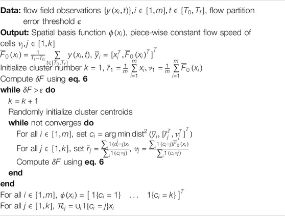
ALGORITHM 1. Flow Field Partition Algorithm
To implement the K-means algorithm, we start by randomly selecting k cell centroids, and then use Lloyd iterations to solve the optimization problem. The Lloyd iteration contains two steps, first assign the points that are closest to a centroid to that centroid, and then recompute the cell centroid. These two steps are repeated until cell membership no longer changes. The K-means algorithm requires proper selection of the number of partitioned cells, k, the choice of which affects the path planning performance and flow modeling quality. If the field is divided into too many regions, then it results in a complicated flow structure and potentially increases the computational cost of path planning. On the other hand, dividing the field into too few regions may result in a large error between the true flow field and the modeled flow field, which potentially leads to significant path planning error. Therefore, we introduce an iterative K-means algorithm that can guarantee a bounded flow field partition error, and at the same time utilize the smallest number of partition regions.
Let
Given an initialized k, we will iteratively perform the K-means algorithm (lines 8, 9), and check if the flow partition error satisfies
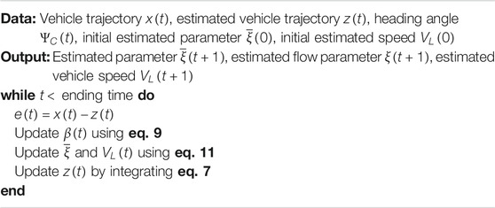
ALGORITHM 2. Flow Estimation Algorithm
Now let us explain Algorithm 2. An estimate
where
The CLLE dynamics can be derived from eqs 7, 1.
We design the learning parameter injection as
and hence the CLLE dynamics becomes
The learning algorithm updates parameters
These rules are then used in Algorithm 2.
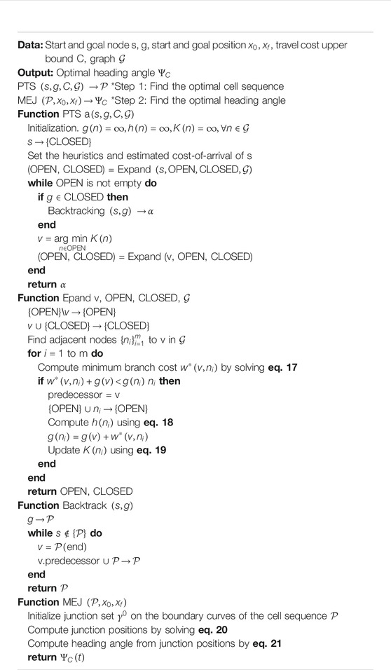
ALGORITHM 3. Bounded Cost Search in Piece-wise Constant Flow Field
4 Bounded Cost Path Planning
Given the piece-wise constant flow model described in eq. 3, the domain is divided into a finite number of regions
Let
From eq. 12, we can represent the vehicle’s heading angle as a function of the junction points,
The vehicle’s travel time in
Combining eq. 14 and eq. 12 we can write the travel time in cell
eq. 15 describes the travel time in one single cell. Based on the discussion of the one cell case, next we talk about solving eq. 4 across multiple cells.
Let
Now let us explain the proposed solution to eq. 16. The solution is presented in Algorithm 3. We propose a bounded cost path planning algorithm that solves for the path that is most likely to satisfy the bounded cost constraint. The solution contains two steps, the first step is solving for the optimal sequence of cells that is most likely to result in a bounded cost path, in the discretized flow map described by the piece-wise constant flow cells. In this step, the junction positions are unknown. An informed graph search method is used for the first step of the proposed solution. The second step is optimizing junction positions on the boundaries of the optimal cell sequence.
The proposed solution is presented in Algorithm 3. First we describe the first step of our solution. Consider having a candidate junction on boundaries of all cells. Two junctions
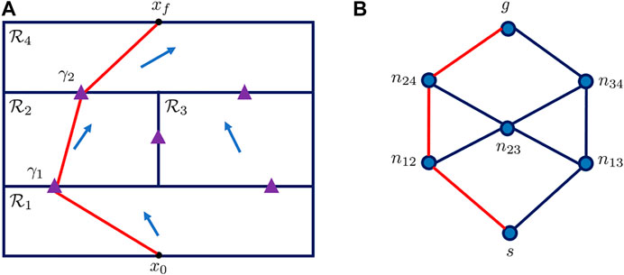
FIGURE 1. (A) Partitioned cells in the domain. On each boundary of two adjacent cells there is a candidate junction point, represented as the purple triangle (B) Graph representation of the workspace. The vertices represent the candidate junctions, while the edges are the path segment between the adjacent junctions. The red line on both of the plots represent the same example path.
The branch cost of the graph is defined as the travel time from one junction to another adjacent junction. The travel time can be computed by eq. 15 if the two junction positions are known. However, since the junction positions are unknown when optimizing the cell sequence, the branch cost of the graph cannot be explicitly computed. Hence we introduced the following assumption:
Assumption 4.1: We assume that the branch cost for all edges in
Remark 4.1: Even though the branch cost is unknown, its minimum value can be computed, since the branch cost eq. 15 is convex with respect to
The informed graph search method we propose is an extension to a class of graph search algorithms called potential search (PTS) (Stern et al., 2014). The PTS algorithms can be viewed as modifications to the celebrated A* algorithm for path planning (Hart et al., 1968). To determine which nodes should be searched, the algorithms maintain an OPEN list and a CLOSED list. A graph node is labeled NEW if it has not been searched by the algorithm. The OPEN list contains all the nodes that are searched, but still have a NEW neighbor. The CLOSED list consists of all the nodes that have been accessed by the search algorithm.To determine which cells should be searched first by the algorithm, the algorithm computes the cost-of-arrival, which is the minimal cost of going from the starting node s to an arbitrary node n, and cost-to-go, which is the minimal cost of going from n to the goal point g. Let
The heuristic function defined in eq. 18 is the travel time of the vehicle traveling in the most favorable flow condition, reaching goal position from the junction position that is closest to the goal. Hence,
Definition 4.1: The potential of a node n, denoted as
This optimization problem is solved by the interior-point method.The optimal heading angle can be computed from the junction positions using eq. 12. In each cell of the sequence
5 Theoretical Justification
In this section, we give theoretical justification to the proposed data-driven flow modeling and bounded cost path planning method.
5.1 Data-Driven Flow Modeling
Algorithm 1 can be theoretically justified by proving that the optimal solution to eq. 5 is the optimal solution to eq. 2. We also prove that Algorithm 2 achieves error convergence and parameter convergence, indicating that the estimated trajectory converges to the actual trajectory, and the estimated parameter converges to the true values.
Lemma 5.1: The optimal flow partition derived by solving eq. 2 is the same as the optimal flow partition derived from eq. 5. PROOF: Let
The second term in J represents the temporal variation of flow speed on one grid point, which does not change with respect to the partitioning of the flow field. Hence
Definition 5.2: (Sastry and Bodson, 1994; Khalil, 1996) A vector signal
The persistent excitation condition is critical to prove the convergence of parameters (Narendra and Annaswamy, 1989). When
Lemma 5.3: The signal vector
Thus
If
Theorem 5.4: Under the updating law eq. 11, CLLE converges to zero when time goes to infinity. PROOF: Consider the following Lyapunov function,
Since
Thus
Theorem 5.5: Under the updating law eq. 11, if the vehicle visits all the partitioned cells,
We define a new state variable
where
There exists some
which is negative semi-definite.Then by the Lyapunov theorem (Theorem 3.8.4 in (Ioannou and Sun, 1995)),
Thus, we now consider the observability of
Let
Due to the assumption that the vehicle visits all cells, by Lemma 5.3,
5.2 Bounded Cost Path Planning
In this subsection, we prove that Algorithm 3 finds the optimal solution of eq. 4. Assumption 5.1 and Assumption 5.2 are required for the optimality proof.
Assumption 5.1: Consider any node not the starting node s or the goal node g, the estimated cost-of-arrival
Remark 5.1: For any node that is not the goal node,
Assumption 5.2: The true cost-to-go,
Remark 5.2: Both
Lemma 5.6: For all
Terms in the above inequality can be computed by integration of the probability density function,
where
which implies
FIGURE 2. Illustration of computing
Lemma 5.7: The optimal path minimizes
Theorem 5.8: When a feasible solution exists, the proposed algorithm terminates if and only if an optimal path is found. PROOF: Algorithm 3 can only terminate by finding the goal node, or after depleting the OPEN set. However, the OPEN set can never be empty before termination if there is a feasible path from s to goal point. Hence Algorithm 3 must terminate by finding a goal point.Next we show that Algorithm 3 terminates only by finding an optimal path to the goal node. Suppose that the algorithm terminates by finding a path,
5.3 Complexity Analysis
In our analysis, we derive the worst case running time for Algorithm 3, and compare it with dynamic programming based planning methods, such as A*, to demonstrate the computational efficiency of the proposed planning algorithm. Let us suppose the flow field forecast is available on
To derive the worst case running time of the proposed algorithm, we first consider the partitioning. Since one junction must be formed by the boundary of at least two cells, the total number of junctions cannot exceeds
The worst case running time of A* is
6 Experiment and Simulation Results
In this section, we provide the results of the implementation of our flow field modeling and path planning methods in a simulated experiment. First, we describe the simulated experimental set-up and recent field experiments, which serve as a strong test of the methods due to the magnitude and variability of the flow. We validate the proposed flow modeling algorithm by comparing the estimated flow model parameters generated from the proposed flow estimation algorithm with the glider estimated flow collected during the experiment. Based on the estimated flow model, simulation of the bounded cost path planning algorithm is performed, and its performance is compared with other AUV path planning algorithms.
6.1 Experimental and Simulation Setup
Our study is motivated by the use of underwater gliders off the coast near Cape Hatteras, North Carolina, US as part of a 16-months experiment (Processes driving Exchange At Cape Hatteras, PEACH) to study the processes that cause exchange between the coastal and deep ocean at Cape Hatteras, a highly dynamic region characterized by confluent western boundary currents and convergence in the adjacent shelf and slope waters. Underwater gliders, AUVs that change their buoyancy and center of mass to “fly” in a sawtooth-shaped pattern, were deployed on the shelf and shelf edge to capture variability in the position of the Hatteras Front, the boundary between cool, fresh water on the shelf of the Mid Atlantic Bight and the warmer, saltier water observed in the South Atlantic Bight.
While the energy efficiency of the glider’s propulsion mechanism permits endurance of weeks to months, the forward speed of the vehicles is fairly limited (0.25–0.30 m/s), which can create significant challenges for navigation in strong currents. Use of a thruster in a so-called “hybrid” glider configuration can increase forward speed to approximately 0.50 m/s, but at great energetic cost. The continental shelf near Cape Hatteras is strongly influenced by the presence of the Gulf Stream, which periodically intrudes onto the shelf, resulting in strong and spatially variable flow that can be nearly an order of magnitude greater than the forward speed of the vehicle (2+ m/s). With realistic estimates of the spatial and temporal variability of the flow, path planning can provide a significant advantage for successful sampling.
We deployed one glider off Oregon Inlet, NC May 16, 2017 and recovered it 14 days later. For its mission, the glider was initially tasked to sample along a path with offshore, inshore, and triangular segments designed to sample critical flow features (Figure 3), and was not used with a thruster. The glider surfaced approximately every 4 h to update its position with a GPS fix, communicate with shore, transmit a subset of data, and most importantly, receive mission updates and commands to adapt sampling.
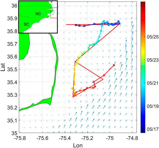
FIGURE 3. Survey domain near Cape Hatteras. The curve represents glider trajectory during the first PEACH deployment. The red line path is the pre-assigned sampling pattern. Squares denote the glider surfacing positions along trajectory, and color of the trajectory depicts timestamps. The arrows represent the NCOM-predicted flow field at the starting time of the deployment.
6.2 Flow Modeling Using Glider Experimental Data
In this example, we present flow modeling results using the proposed flow partition and parameter estimation methods.
The flow map forecast is given by a 1-km horizontal resolution version of the Navy Coastal Ocean Model (NCOM, Martin, 2000), made available by J. Book and J. Osborne (Naval Research Laboratory, Stennis Space Center, United States). In the domain of interest, the ocean model flow forecast is given at
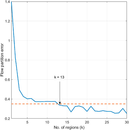
FIGURE 4. Flow partition error when the number of cells is set as
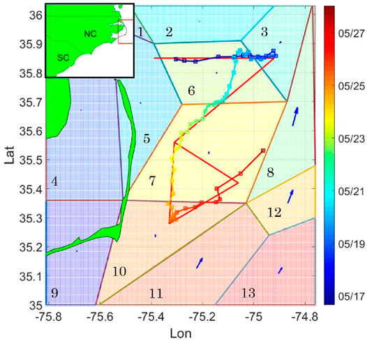
FIGURE 5. Partitioned cells of the survey domain. The polygons are the partitioned regions. The blue arrows represent uniform flow speed in each of the cells generated from the proposed algorithm.
At each surfacing, the vehicle position is given by the GPS location. When the glider is underwater, we use linear interpolation to estimate the heading and vehicle position. The vehicle’s forward speed is zero when it is at the surface of the ocean, and the vehicle drifts freely with the surface current. This violates the constant forward speed assumption stated in Assumption 2.1. Hence, we remove the segment of data when the vehicle is drifting at surface, and then compute the estimated flow parameters by the proposed algorithm. Glider speed is initialized to be 0.3 m/s, while the flow parameters are initialized by the flow vectors found by partitioning the NCOM data. Since the vehicle trajectory crosses cell 3, 6, 7, 10, and does not enter other cells, the glider trajectory does not satisfy persistent excitation condition described in Lemma 5.3. Hence only the flow parameters in cells 3, 6, 7, 10 can be updated by the adaptive updating law, while the flow parameters in the rest cells remain to be the initial value. To justify performance of the proposed flow parameter estimation algorithm, we use the ADCIRC (Advanced Circulation) model output (Luettich et al., 1992) to model the tidal flow component, and derive the non-tidal glider estimated flow speed by subtracting ADCIRC reported flow from the flow parameter estimate. The de-tided glider estimated flow speed is considered as the ground truth of flow parameters in the corresponding cells. The root mean square error (rmse) between the estimated parameter and the ground truth in cell 3, 6, 7, 10 is shown in Table 1. It can be seen that in all of the four cells, the estimated flow parameters is in good agreement with the true flow parameters. The rmse in all of the four cells is within
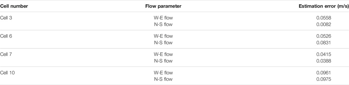
TABLE 1. Root mean square error between the estimated and the true flow parameters.

FIGURE 6. Estimated flow parameters and the ground truth value in cell 7.
6.3 Bounded Cost Path Planning
In this example, we present simulation results of AUV bounded cost path planning. Since the flow field is of high speed in the domain of interest, we assume that the glider is sampling the domain using combined propulsion of buoyancy and thrusters for the operation. Hence the AUV through-water speed is set to be 0.5 m/s. The simulations are run on a core i7 at 1.80 GHz PC with 32GB RAM.
Figure 7 shows one example of the proposed bounded cost path planning method. The start position and goal position is assigned as
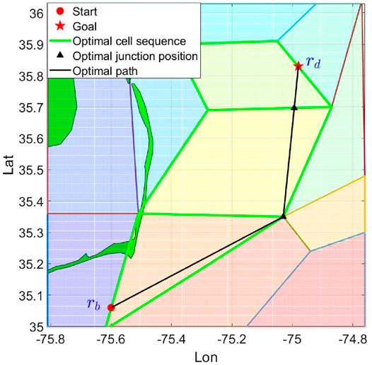
FIGURE 7. Example of simulation case. The resulting path is computed by the proposed method.
We perform A* (Carroll et al., 1992) and Level Set Method (LSM) (Lolla et al., 2014) as comparison to the proposed method. 15 test cases are generated in total. Each test case
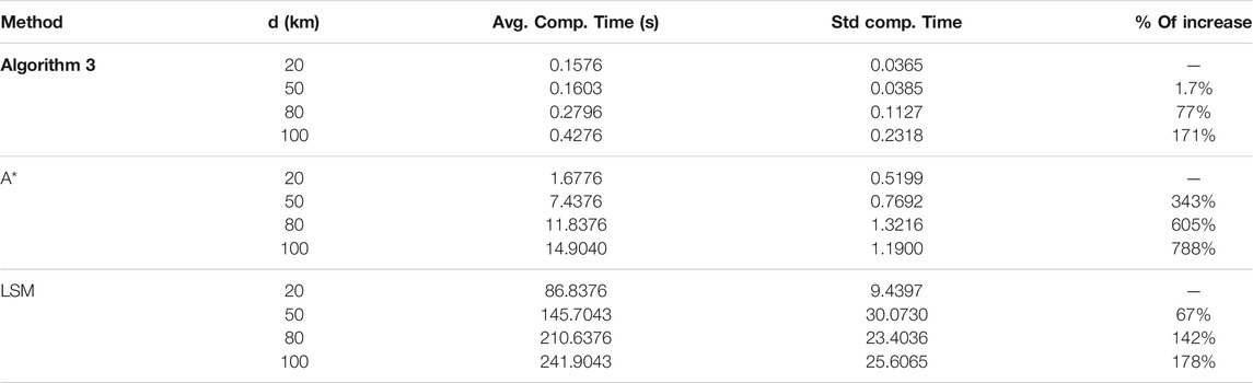
TABLE 2. Computation time comparison of A*, Level Set Method, and the proposed algorithm. Avg. comp. time represents the averaged computation time for each simulation scenario, and STD comp. time represents the standard deviation of the computation time.
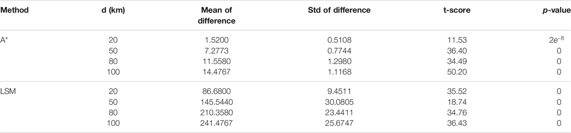
TABLE 3. Post-hoc analysis of simulation comparison between the proposed method, A*, and LSM. The mean and STD of difference describe the mean and standard deviation of the computation time difference between the proposed method and the two other methods. The significance level is set as
Further, we compare the percentage of increase in the computation time when d increases. In Table 2, the
It is worth mentioning that the proposed algorithm achieves decreased computation cost by compromising the path quality. Even though optimality of the planned path is guaranteed in the partitioned flow field, as shown in Theorem 5.8, the planned path may not be optimal in the actual flow field, since the partitioned flow field is different from the actual flow field. We identify the compromised path quality as the major constraint of the proposed algorithm.
In cases where the domain is larger, Algorithm 1 may still result in large number of cells, leading to increased computation cost in solving the bounded cost planning problem. In such scenarios, stochastic optimization methods, such as the differential evolution method, may be helpful in further reducing the computation cost of solving the planning problem. We refer to a survey paper on the differential evolution methods (Das et al., 2016) for this matter.
7 Conclusion
In this paper, a bounded cost path planning method is developed for underwater vehicles assisted by a data driven flow field modeling method. The main advantage of the proposed modified PTS method is that it is more computational efficient comparing to A* and LSM in solving AUV planning problem in time-invariant 2D fields, as demonstrated by the simulation result. Major limitation of the proposed algorithm is the compromised solution quality, resulting from the model reduction error introduced by the flow partition process. The proposed method has the potential to be extended to other path planning applications where the task performance is sensitive to planner’s computational efficiency. Future work will include performing the proposed method in real glider deployments, to compare the planned trajectory with the real mission trajectory, where drift and time-varying fields happen. Future work will also include comparing the proposed method with other algorithms, such as the differential evolution algorithms.
Data Availability Statement
Publicly available datasets were analyzed in this study. This data can be found here: https://www.ncdc.noaa.gov/data-access/model-data/model-datasets/navoceano-ncom-reg. The flow map data analyzed in this work is given by the Navy Coastal Ocean Model made available by J. Book and J. Osborne of Naval Research Laboratory, Stennis Space Center, US.
Author Contributions
MH, SC, and FZ contributed to design and theoretical analysis of the methods, and wrote the first draft of the manuscript. HZ, CE and FZ wrote sections of the manuscript and provided guidance for the research work. All authors contributed to the manuscript revision, read, and approved the submitted version.
Conflict of Interest
The authors declare that the research was conducted in the absence of any commercial or financial relationships that could be construed as a potential conflict of interest.
References
Carroll, K. P., McClaran, S. R., Nelson, E. L., Barnett, D. M., Friesen, D. K., and Williams, G. N. (1992). “AUV Path Planning: An A* Approach to Path Planning with Consideration of Variable Vehicle Speeds and Multiple, Overlapping, Time-Dependent Exclusion Zones,” in Proceedings of the 1992 Symposium on Autonomous Underwater Vehicle Technology.
Chang, D., Liang, X., Wu, W., Edwards, C. R., and Zhang, F. (2014). Real-time Modeling of Ocean Currents for Navigating Underwater Glider Sensing Networks. Coop. Robots Sensor Networks, Stud. Comput. Intelligence 507, 61–75. doi:10.1007/978-3-642-39301-3_4
Chang, D., Zhang, F., and Edwards, C. R. (2015). Real-Time Guidance of Underwater Gliders Assisted by Predictive Ocean Models. J. Atmos. Oceanic Tech. 32, 562–578. doi:10.1175/jtech-d-14-00098.1
Chassignet, E. P., Hurlburt, H. E., Smedstad, O. M., Halliwell, G. R., Hogan, P. J., Wallcraft, A. J., et al. (2007). The HYCOM (HYbrid Coordinate Ocean Model) Data Assimilative System. J. Mar. Syst. 65, 60–83. doi:10.1016/j.jmarsys.2005.09.016
Cho, S., and Zhang, F. (2016). “An Adaptive Control Law for Controlled Lagrangian Particle Tracking,” in Proceedings of the 11th ACM International Conference on Underwater Networks & Systems, 1–5.
Cho, S., Zhang, F., and Edwards, C. R. (2021). Learning and Detecting Abnormal Speed of marine Robots. Int. J. Adv. Robotic Syst. 18, 1729881421999268. doi:10.1177/1729881421999268
Cui, R., Li, Y., and Yan, W. (2015). Mutual Information-Based Multi-AUV Path Planning for Scalar Field Sampling Using Multidimensional RRT. IEEE Trans. Syst. Man, Cybernetics: Syst. 46, 993–1004.
Das, S., Mullick, S. S., and Suganthan, P. N. (2016). Recent Advances in Differential Evolution - an Updated Survey. Swarm Evol. Comput. 27, 1–30. doi:10.1016/j.swevo.2016.01.004
Eichhorn, M. (2013). Optimal Routing Strategies for Autonomous Underwater Vehicles in Time-Varying Environment. Robotics and Autonomous Systems. 67, 3–43. doi:10.1016/j.robot.2013.08.010
Gammell, J. D., Barfoot, T. D., and Srinivasa, S. S. (2018). Informed Sampling for Asymptotically Optimal Path Planning. IEEE Trans. Robot. 34, 966–984. doi:10.1109/tro.2018.2830331
Griffa, A., Piterbarg, L. I., and Özgökmen, T. (2004). Predictability of Lagrangian Particle Trajectories: Effects of Smoothing of the Underlying Eulerian Flow. J. Mar. Res. 62, 1–35. doi:10.1357/00222400460744609
Haidvogel, D. B., Arango, H., Budgell, W. P., Cornuelle, B. D., Curchitser, E., Di Lorenzo, E., et al. (2008). Ocean Forecasting in Terrain-Following Coordinates: Formulation and Skill Assessment of the Regional Ocean Modeling System. J. Comput. Phys. 227, 3595–3624. doi:10.1016/j.jcp.2007.06.016
Hart, P., Nilsson, N. J., and Raphael, B. (1968). A Formal Basis for the Heuristic Determination of Minimum Cost Paths. IEEE Transaction of Systems Science and Cybernetics SSC, 4.
Haza, A. C., Piterbarg, L. I., Martin, P., Özgökmen, T. M., and Griffa, A. (2007). A Lagrangian Subgridscale Model for Particle Transport Improvement and Application in the Adriatic Sea Using the Navy Coastal Ocean Model. Ocean Model. 17, 68–91. doi:10.1016/j.ocemod.2006.10.004
Hou, M., Zhai, H., Zhou, H., and Zhang, F. (2019). “Partitioning Ocean Flow Field for Underwater Vehicle Path Planning,” in OCEANS 2019-Marseille (IEEE), 1–8.
Karaman, S., and Frazzoli, E. (2011). Sampling-based Algorithms for Optimal Motion Planning. Int. J. Robotics Res. 30, 846–894. doi:10.1177/0278364911406761
Kim, S.-J., Koh, K., Lustig, M., Boyd, S., and Gorinevsky, D. (2007). An Interior-Point Method for Large-Scale-Regularized Least Squares. IEEE J. Sel. Top. Signal. Process. 1, 606–617. doi:10.1109/JSTSP.2007.910971
Kuffner, J. J., and LaValle, S. M. (2000). “RRT-connect: An Efficient Approach to Single-Query Path Planning,” in Proceedings 2000 ICRA. Millennium Conference. IEEE International Conference on Robotics and Automation (Symposia Proceedings (Cat. No. 00CH37065) (IEEE)), 995–1001.
Kularatne, D., Bhattacharya, S., and Hsieh, M. A. (2018). Going with the Flow: a Graph Based Approach to Optimal Path Planning in General Flows. Auton. Robot 42, 1369–1387. doi:10.1007/s10514-018-9741-6
Kularatne, D., Bhattacharya, S., and Hsieh, M. A. (2017). Optimal Path Planning in Time-Varying Flows Using Adaptive Discretization. IEEE Robotics Automation Lett. 3, 458–465.
Leonard, N. E., Paley, D. A., Davis, R. E., Fratantoni, D. M., Lekien, F., and Zhang, F. (2010). Coordinated Control of an Underwater Glider Fleet in an Adaptive Ocean Sampling Field experiment in Monterey Bay. J. Field Robotics 27, 718–740. doi:10.1002/rob.20366
Lermusiaux, P. F. J. (2006). Uncertainty Estimation and Prediction for Interdisciplinary Ocean Dynamics. J. Comput. Phys. 217, 176–199. doi:10.1016/j.jcp.2006.02.010
Li, W., Lu, J., Zhou, H., and Chow, S.-N. (2017). Method of Evolving Junctions: A New Approach to Optimal Control with Constraints. Automatica 78, 72–78. doi:10.1016/j.automatica.2016.12.023
Lolla, T., Lermusiaux, P. F. J., Ueckermann, M. P., and Haley, P. J. (2014). Time-optimal Path Planning in Dynamic Flows Using Level Set Equations: Theory and Schemes. Ocean Dyn. 64, 1373–1397. doi:10.1007/s10236-014-0757-y
Luettich, R. A., Westerink, J. J., Scheffner, N. W., et al. (1992). ADCIRC: an advanced three-dimensional circulation model for shelves, coasts, and estuaries. Report 1, Theory and methodology of ADCIRC-2DD1 and ADCIRC-3DL. Tech. rep., Coastal Engineering Research Center, Mississippi, US.
Martin, P. J. (2000). Description of the Navy Coastal Ocean Model Version 1.0. Tech. Rep. NRL/FR/7322–67900-9962. Mississippi, US: Naval Research Lab Stennis Space Center.
Mokhasi, P., Rempfer, D., and Kandala, S. (2009). Predictive Flow-Field Estimation. Physica D: Nonlinear Phenomena 238, 290–308. doi:10.1016/j.physd.2008.10.009
Ozog, P., Carlevaris-Bianco, N., Kim, A., and Eustice, R. M. (2016). Long-term Mapping Techniques for Ship hull Inspection and Surveillance Using an Autonomous Underwater Vehicle. J. Field Robotics 33, 265–289. doi:10.1002/rob.21582
Panda, M., Das, B., Subudhi, B., and Pati, B. B. (2020). A Comprehensive Review of Path Planning Algorithms for Autonomous Underwater Vehicles. Int. J. Autom. Comput. 17, 321–352. doi:10.1007/s11633-019-1204-9
Pereira, A. A., Binney, J., Hollinger, G. A., and Sukhatme, G. S. (2013). Risk-aware Path Planning for Autonomous Underwater Vehicles Using Predictive Ocean Models. J. Field Robotics 30, 741–762. doi:10.1002/rob.21472
Rhoads, B., Mezic, I., and Poje, A. C. (2012). Minimum Time Heading Control of Underpowered Vehicles in Time-Varying Ocean Currents. Ocean Eng. 66, 12–31.
Roberge, V., Tarbouchi, M., and Labonté, G. (2012). Comparison of Parallel Genetic Algorithm and Particle Swarm Optimization for Real-Time UAV Path Planning. IEEE Trans. Ind. Inform. 9, 132–141.
Sastry, S., and Bodson, M. (1994). Adaptive Control: Stability, Convergence and Robustness. New Jersey, US: Prentice-Hall.
Savidge, D. K., Austin, J. A., and Blanton, B. O. (2013a). Variation in the Hatteras Front Density and Velocity Structure Part 1: High Resolution Transects from Three Seasons in 2004-2005. Continental Shelf Res. 54, 93–105. doi:10.1016/j.csr.2012.11.005
Savidge, D. K., Austin, J. A., and Blanton, B. O. (2013b). Variation in the Hatteras Front Density and Velocity Structure Part 2: Historical Setting. Continental Shelf Res. 54, 106–116. doi:10.1016/j.csr.2012.11.006
Shchepetkin, A. F., and McWilliams, J. C. (2005). The Regional Oceanic Modeling System (ROMS): a Split-Explicit, Free-Surface, Topography-Following-Coordinate Oceanic Model. Ocean Model. 9, 347–404. doi:10.1016/j.ocemod.2004.08.002
Smith, R. N., Chao, Y., Li, P. P., Caron, D. A., Jones, B. H., and Sukhatme, G. S. (2010). Planning and Implementing Trajectories for Autonomous Underwater Vehicles to Track Evolving Ocean Processes Based on Predictions from a Regional Ocean Model. Int. J. Robotics Res. 29, 1475–1497. doi:10.1177/0278364910377243
Soulignac, M. (2011). Feasible and Optimal Path Planning in strong Current fields. IEEE Trans. Robot. 27, 89–98. doi:10.1109/tro.2010.2085790
Stern, R., Felner, A., van den Berg, J., Puzis, R., Shah, R., and Goldberg, K. (2014). Potential-based Bounded-Cost Search and Anytime Non-parametric A*. Artif. Intelligence 214, 1–25. doi:10.1016/j.artint.2014.05.002
Stern, R. T., Puzis, R., and Felner, A. (2011). “Potential Search: A Bounded-Cost Search Algorithm,” in Twenty-First International Conference on Automated Planning and Scheduling.
Subramani, D. N., and Lermusiaux, P. F. J. (2016). Energy-optimal Path Planning by Stochastic Dynamically Orthogonal Level-Set Optimization. Ocean Model. 100, 57–77. doi:10.1016/j.ocemod.2016.01.006
Thayer, J. T., Stern, R., Felner, A., and Ruml, W. (2012). “Faster Bounded-Cost Search Using Inadmissible Estimates,” in Twenty-Second International Conference on Automated Planning and Scheduling.
Xiang, X., Jouvencel, B., and Parodi, O. (2010). Coordinated Formation Control of Multiple Autonomous Underwater Vehicles for Pipeline Inspection. Int. J. Adv. Robotic Syst. 7, 3. doi:10.5772/7242
Zamuda, A., Hernández Sosa, J. D., and Adler, L. (2016). Constrained Differential Evolution Optimization for Underwater Glider Path Planning in Sub-mesoscale Eddy Sampling. Appl. Soft Comput. 42, 93–118. doi:10.1016/j.asoc.2016.01.038
Zamuda, A., and Hernández Sosa, J. D. (2014). Differential Evolution and Underwater Glider Path Planning Applied to the Short-Term Opportunistic Sampling of Dynamic Mesoscale Ocean Structures. Appl. Soft Comput. 24, 95–108. doi:10.1016/j.asoc.2014.06.048
Zamuda, A., and Sosa, J. D. H. (2019). Success History Applied to Expert System for Underwater Glider Path Planning Using Differential Evolution. Expert Syst. Appl. 119, 155–170. doi:10.1016/j.eswa.2018.10.048
Zeng, Z., Lammas, A., Sammut, K., He, F., and Tang, Y. (2014). Shell Space Decomposition Based Path Planning for AUVs Operating in a Variable Environment. Ocean Eng. 91, 181–195. doi:10.1016/j.oceaneng.2014.09.001
Zeng, Z., Lian, L., Sammut, K., He, F., Tang, Y., and Lammas, A. (2015). A Survey on Path Planning for Persistent Autonomy of Autonomous Underwater Vehicles. Ocean Eng. 110, 303–313. doi:10.1016/j.oceaneng.2015.10.007
Zhai, H., Hou, M., Zhang, F., and Zhou, H. (2020). Method of Evolving junction on Optimal Path Planning in Flow fields. IEEE Transactions on Robotics.
Keywords: robotic path planning, graph search method, bounded cost search, parameter identification, underwater vehicle
Citation: Hou M, Cho S, Zhou H, Edwards CR and Zhang F (2021) Bounded Cost Path Planning for Underwater Vehicles Assisted by a Time-Invariant Partitioned Flow Field Model. Front. Robot. AI 8:575267. doi: 10.3389/frobt.2021.575267
Received: 23 June 2020; Accepted: 17 June 2021;
Published: 14 July 2021.
Edited by:
Victor Zykov, Independent researcher, Menlo Park, CA, United StatesReviewed by:
Navid Razmjooy, Independent researcher, Ghent, BelgiumGuangjie Han, Hohai University, China
Copyright © 2021 Hou, Cho, Zhou, Edwards and Zhang. This is an open-access article distributed under the terms of the Creative Commons Attribution License (CC BY). The use, distribution or reproduction in other forums is permitted, provided the original author(s) and the copyright owner(s) are credited and that the original publication in this journal is cited, in accordance with accepted academic practice. No use, distribution or reproduction is permitted which does not comply with these terms.
*Correspondence: Fumin Zhang, ZnVtaW5AZ2F0ZWNoLmVkdQ==