Estimating Hidden Markov Models (HMMs) of the cognitive process in strategic thinking using eye-tracking

Hidden Markov Models (HMMs) are used to study language, sleep, macroeconomic states, and other processes that reflect probabilistic transitions between states that can't be observed directly. This paper applies HMMs to data from location-based game theory experiments. In these location games, players choose a pixel location from an image. These players either have a common goal (choose a matching location), or competing goals, to mismatch (hide) or match (seek) in hider-seeker games. We use eye-tracking to record where players look throughout the experimental decision. Each location's numerical salience is predicted using an accurate, specialized vision science-based neural network [the Saliency Attentive Model (SAM)]. The HMM shows the pattern of transitioning from hidden states corresponding to either high or low-salience locations, combining the eye-tracking and salience data. The transitions vary based on the player's strategic goal. For example, hiders transition more often to low-salience states than seekers do. The estimated HMM is then used to do two useful things. First, a continuous-time HMM (cHMM) predicts the salience level of each player's looking over several seconds. The cHMM can then be used to predict what would happen if the same process was truncated by time pressure: This calculation makes a specific numerical prediction about how often seekers will win, and it predicts an increase in win rate but underestimates the size of the change. Second, a discrete-time HMM (dHMM) can be used to infer levels of strategic thinking from high-to-low salience eye-tracking transitions. The resulting estimates are more plausible than some maximum-likelihood models, which underestimate strategic sophistication in these games. Other applications of HMM in experimental economics are suggested.

1. Introduction

Behavioral game theory is a collection of theories and evidence about how biological limits on perception, strategic thinking, and stochastic response affect behavior in strategic games. In this study, we combine elements of two behavioral approaches in a new way. The first approach is a cognitive hierarchy of “level-k” thinkers in games. The second approach makes use of eye-tracking data, recording where participants look on a computer screen at a high temporal frequency to infer their choice process.

We combine the level-k approach and eye-tracking data to fit a “Hidden Markov Model” (HMM). Our hidden layer is the mental states (or internal beliefs) of the player which are statistically inferred from observations. The Markov property means that the evolution of the process in the future depends only on the present state and does not depend on history (this is a simplification used in many areas of economic theory and is usually a good approximation).

These HMM models are within a class of dynamic models also used in many areas of applied economics. Most dynamic models adopt a Markov assumption for simplicity. When an unobserved state variable is thought to be a crucial driver of behavior, researchers look for a proxy of that. The proxy is typically assumed to be locally independent of everything else, in which case those dynamic models are also HMMs (Cunha et al., 2010; Arrelano et al., 2017; Hu, 2017; Hu et al., 2017). The major difference in the application of HMM to experimental data, compared to these very general dynamic selection models, is that experimental control usually allows a much better selection of proxy variables for hidden states.

In the games we analyze, HMMs are used to summarize the dynamics of the cognitive process in thinking and choice selection. HMMs enable us to see, for example, how hiders and seekers in a hider-seeker game shift their attention differently. In addition, the HMMs are used in two new types of analyses. The first new analysis is to estimate the frequency distribution of level types, based on between-state transitions. This is a novel way to estimate level types (though related to Costa-Gomes et al., 2001) and can be done for individual-game trial-by-trial data, then aggregated.

The second new analysis is the development of a continuous-time version of HMM which creates a time series of the mental states players enter throughout a game. In our experiment, mental states refers to the player believing they are in a “high” or “low” saliency location. This HMM can be used to predict the effect time pressure may have on behavior–roughly speaking, are players further from equilibrium when they have less time to choose? We find that the answer is Yes but, more importantly, our continuous HMM makes a quantitative prediction for the magnitude of the behavioral statistic (the frequency of matching in hider-seeker games under time pressure). This type of specific prediction from one game to a time-pressured one is unusual in model-based experimental economics.

2. Background

In this section, we describe the motivation and milestones in combining level-k modeling, eye-tracking, and HMM for use in economics.

Many previous studies have analyzed how level-k type models work (Stahl and Wilson, 1994; Nagel, 1995; Camerer et al., 2004; Kübler and Weizsäcker, 2004; Crawford and Iriberri, 2007b; Kneeland, 2015; Alaoui and Penta, 2016; Friedenberg et al., 2016; Brandenburger et al., 2017; Alaoui et al., 2020). Our approach is loosely related to these contributions. Our HMM structure is general, so it is not guaranteed to recover transitions between mental states which correspond to levels of strategic thinking. However, if the unconstrained structure indicates level-k-type transitions, that is promising evidence that such theories are on the right track.

In the last couple of decades, starting with Camerer et al. (1993), experimental economists began to use “process” data, along with choice data, to understand the cognitive process of human strategic play. The most difficult way to study the cognitive process has been to measure human brain activity directly (Bhatt and Camerer, 2005; Hampton et al., 2008; Coricelli and Nagel, 2009; Ong et al., 2018; Mi et al., 2021). A simpler way is to use choice process data that can be collected at low marginal cost, such as response times, and eye gaze or mouse movement recordings (Camerer et al., 1993, 2004; Costa-Gomes et al., 2001; Wang et al., 2010; Brocas et al., 2014; Polonio et al., 2015; Devetag et al., 2016). These choice process data provide better evidence of a participant's thought process than those from choices alone (Fudenberg and Levine, 2016, p. 9). This improvement becomes clear when one considers the following scenario: Suppose a careless player in an experiment testing for mixed-strategy equilibrium does not read the instructions describing the game structure carefully and chooses haphazardly. This player may make a series of varying choices that look similar to those of a sophisticated player who is approximating a mixed strategy with a more thoughtful process. Differentiating between these two players based solely only on their choices or response times might be difficult. However, the addition of eye-tracking data should enable a researcher to easily differentiate these two participants, as eye movements of the sophisticated player may show the player glancing at a sequence of payoffs consistent with level-type thinking as opposed to the careless player who may look around more erratically or hardly look at payoffs at all.

Early attempts at differentiating thought processes from two players with similar choice data in games, but distinct strategies, made use of fixation times and choice frequencies. For example, Camerer et al. (1993) and Johnson et al. (2002) found that in three-stage alternating-offer bargaining games, most players did not look at the third-stage payoffs (as is required to choose equilibrium strategies). Visual patterns were correlated with deviations from predicted bargaining offers. Carillo and Brocas (2003) found that choices in games with forward induction were associated with payoff lookups.

A deeper attempt at distinguishing level 1 (L1) play and D1 play came from Costa-Gomes et al. (2001). L1 play is maximizing the expected value against a random player. D1 play is similar to L1 but assumes the opponent does not play a dominated strategy. D1 maximizes the expected values against a player who is not entirely random because she never plays dominated strategies. L1 and D1 strategies lead to similar choices in many games. But even when L1 and D1 predict the same choice, they can be distinguished by mouse-tracking measures of what payoffs players fixate on. The D1 choices requires looking at the other player's payoff and the L1 choice does not. In their study, Costa-Gomes found that there were significantly more D1 players than L1 players.

After this first wave of studies, more sophisticated types of analyses were developed to use both look-ups of specific payoffs and transitions between payoffs (called “saccades” in visual science) to infer the decision rules players appeared to use (Costa-Gomes and Crawford, 2006). Many of these second-wave studies made use of eye-tracking data, captured by a camera-based recording of temporally fine-grained (25 ms) visual fixations to items on a computer screen (Costa-Gomes et al., 2001; Wang et al., 2010; Polonio et al., 2015; Devetag et al., 2016). Inference from payoff comparison has added substantial choice process evidence. Costa-Gomes et al. (2001) studied the strategic sophistication during normal-form game-plays via mouse lab. In their paper, the authors pre-specify nine behavioral types; including altruistic, pessimistic, optimistic, naive, L2, D1, D2, equilibrium, and sophisticated. These types theoretically determine subjects' information search patterns based on two principles: adjacency and occurrence. This type-based model successfully captures different strategic behaviors for the combination of choice search patterns.

The general finding from these studies is that the decision rules players use are often simple, and often classified into hierarchical levels. However, players do not have a perfect memory and it is often easier to look again than to remember, and are likely to be approximating cognitively demanding rules like dominance detection by lookup shortcuts. Extracting decision rule evidence, therefore, requires specialized econometrics and careful specification of how errors might occur (see Costa-Gomes et al., 2001).

Our paper uses eye-tracking data as in some earlier studies, but fits these data to a “Hidden Markov Model” (HMM). Compared to the previous methods in which behavioral types and patterns need to be pre-specified, the HMM method can automatically infer behavioral types “unsupervised” from the data. HMM is widely used in machine learning and cognitive science, but there are only a small number of previous applications in experimental economics.¹ Hu et al. (2017) used a model with hidden state transitions to compare Bayesian and reinforcement learning in an experimental reversal learning task. They used visual attention to valued stimuli as a proxy for subjective value. Alós-Ferrer and Garagnani (2023) used HMM to study the temporal interplay between different behavioral types such as Bayes or reinforcement when an agent faces binary choice problems. They found that players transit dynamically from the above types when facing a simple choice problem (Ansari et al., 2012).

In HMM the states are “hidden” in the sense that we cannot directly observe what state a person is in.² However, different hidden states and transition probabilities will create different information-acquiring patterns and different choice-generating schemas.

In this paper, we first present the main model of a discrete HMM and how it corresponds to choices in strategic games in Section 3.1. The next section introduces an eye-tracking data set from Li and Camerer (2022). We estimate the proposed model using the eye-tracking data collected and illustrate the new insights the estimated HMM model gives.

In Section 5, we introduce a new level identification method based on a gaze data set and an estimated HMM model. We show the full distribution of levels across different trials, players, and strategic games. An approximately exponential drop in levels is observed, which is consistent with earlier results that people rarely reason more than two levels.

In Section 6, we extend the HMM model to be continuous. The continuous model can include state duration time for each hidden state using fixation duration data. We call it cHMM to distinguish it from the discrete one. The cHMM is dynamic in time and can make new predictions of choices under time pressure. We estimate the cHMM model using the gaze data we have and show predicted strategies of different games at different time points.

The paper ends with a discussion section indicating the limits of the model and other types of experimental questions it could be usefully applied to.

3. HMM and its use in in-game experiments

The games studied in this paper are location games. Two players see a common 2D natural image (Li and Camerer, 2022). Players have a few seconds to choose a pixel in the image (a location) by clicking the region they'd like to select. They choose simultaneously (i.e., without knowing what the other player is choosing or has chosen). The game “strategies” are therefore pixel locations. A circle with a radius of 108 pixels is drawn around their chosen pixel. Figure 1 demonstrates examples of what the circle and images look like. In matching games, players both earn a fixed payoff if the pixel-centered circles overlap (even if only partially). In hider-seeker games, the hider wins from a mismatch (circles do not overlap) and the seeker wins from a match (the circles do overlap).

FIGURE 1

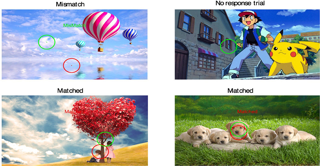
Figure 1. Examples of trial outcomes. In the location game experiment, all games share the same rule of matching that if two circles overlap constitute a successful match. The circles here give out a direct visual effect of how large it is comparing to the rest of an image.

A carefully-trained algorithm [Saliency Attentive Model (SAM)]³ is used to exogenously predict the bottom-up visual salience of each pixel in each image. The salience values for any image are normalized from 0 to 1 uniformly (i.e., the salience values are quantiles).

Bottom-up salience is a concept from cognitive psychology and neuroscience. Bottom-up visual features are low-level features, such as color, orientation, intensity (brightness), centrality, and high-level features such as objects, faces, or animals. The salience is predicted ex-ante, from an algorithm trained on entirely different images and different players. Algorithmic salience is described further below. Figure 2 gives two examples from Li and Camerer (2022) both the visual salience map predicted by the Saliency Attentive Model (SAM) and the actual choices people made in a coordination game features (Cornia et al., 2018).

FIGURE 2

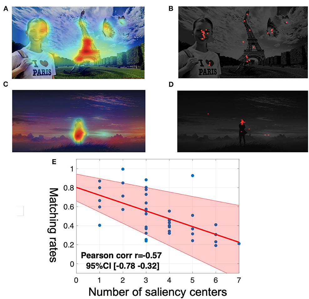
Figure 2. (A) Is an image with seven salience centers^a (C) is an image with one salience center. (B, D) Are corresponding maps (red dots) of actual choice data when people are trying to coordinate. The choice map in (B) is more dispersed because the salience centers in (A) are more numerous. (E) Plots the negative correlation between the number of salience centers and the matching rate. Data is taken from our experiment. ^aSalience center is defined with respect to local maxima of the salience distribution. More salience center will make the image look “busier”.

3.1. The general HMM model

In this section, we describe HMMs and what we can learn about behavioral game theory from them. Our description is very compact and notation-heavy, describing the basic discrete dHMM following a standard framework in Murphy (1998). We also note the critical assumptions that underlie the HMM model. More details are easily found in Frühwirth-Schnatter (2006).

A Hidden Markov Model ℍ = < P, B, Π > is defined as:

• A finite set of states Ω = {h₁, h₂..h_i..h_n}. The number of states n needs to be pre-specified.

• A transition matrix P. Each entry p_ij is the probability of transitioning to state j from the current state i (and the self-transitioning action i = j is included).

• A set of observation states O.

• A projection probability matrix B, mapping the hidden state space elements of Ω to O. The value b_mn is the probability of observation state n conditional on the current hidden state being h_m if the observational space is discrete. Other assumptions will be needed if O is continuous. A popular assumption is to assume the projection is Gaussian distributed (as we do in this paper).

• A n × 1 prior vector Π, indicating the initial probability distribution over states h_i.

Key Assumptions of HMM:

• Independence: Observations x_t are conditionally independent of all other variables given z_t, so the observation at time t depends only on the current state z_t.

• Stationarity: The z_t's form a (first order) Markov chain, i.e.,

• P(z_t ∣ z_t − 1, ..., z₁) = P(z_t ∣ z_t − 1) t = 2,..., T. The chain is also typically assumed to be homogeneous because the transition probabilities do not depend on t.

There are two special states that are different from others. One is the start state S to initiate the game. The other is the end state D, which means a decision is generated. These two states are the only states that are not associated with any fixation, and the end state is associated with choices. The reasoning process that takes a player from S to the hidden states and then finally to D is what the eye-tracking data set used to infer. Note that we classify a player's level-k by the number of transitions (during the hidden states) that the player undergoes during the game, meaning that a player whose transition pattern was HLHL (with H being high salient locations and L being low salient locations) would be considered level-3 while a player that transitioned HHLH would be considered level-2.

Given a fixation data set and game G, a dHMM can be estimated using the Baum-Welch algorithm. Baum-Welch is a special case of the workhorse expectation-maximization algorithm. This process uses available data to “learn” the best-fit transition matrix P and the projection matrix B (for details about the estimation process, Baum et al., 1970; see Appendix).

Our analysis below focuses on an HMM with two hidden states (excluding S and D). One state consists of fixations at locations that have a distribution of low saliency values, classified as state L. In this state, fixations are on locations with lower saliency as measured independently, by the SAM algorithm. Note that SAM generates predictions of salience based purely on the images—no data we collected changes those predictions. The fixations are recorded by the eye-tracker.

In the HMM we estimated for matching games, the mean of the L-state saliency levels is 0.57. That means that for a particular image, there will be many pixel locations, with saliency around 0.57 (Gaussian distributed with mean 0.57 and a variance that is estimated). A fixation is assigned to be in the L state if the saliency of the pixel which the person is looking at is likely to come from that distribution. Note that being “in the L state” is the same, for the HMM, as being at one of the many pixel locations with saliency around 0.57.

The other state is a high-saliency state classified as H. In this state, fixations are on locations with higher saliency (estimated to be a mean of 0.90 in matching games).

Recall that saliency is normalized to be uniformly distributed from 0 to 1 across all pixels in an image. Because the L and H state saliency means are 0.57 and 0.90, it follows that there is a high percentage of low-saliency image locations, with saliency <0.40 or below, which are not part of either state L or H. That's because the fitted model uses the information to derive the states; the model concludes that there are so few fixations to those low-salience pixels that they can be ignored. If such fixations were more common, there would be a better-fitting model including a very-low-salience state; but that's not what the modeling tells us.

Salience levels in L and H are assumed to be drawn from two Gaussian distributions of saliency levels, with the means and accompanying variances of saliency levels within each state estimated from the data. Though our states are “semi-observable,” since we can observe fixations, modeling the hidden states in this method allows the model class to fit as desired.

What is Markovian about HMMs? The Markovian property is the usual one: Transitions out of a current state are assumed to be independent of the sequence of states visited previously. Just as in Markovian analysis of game-theoretic strategies, this simplifies modeling greatly and is likely to be a good approximation (and can also be relaxed to allow higher-order chains, Langeheine and Van de Pol 2000).

HMMs were created by Leonard Baum in the late 1960s, then advanced further at Carnegie-Mellon and IBM. They were first applied to problems of signal processing such as speech recognition—for example, inferring words (hidden states) from observations of spoken phonemes. Rabiner (1989)'s tutorial catalyzed interest (see Juang and Rabiner, 2005, for more history).

HMMs have then been applied to many other domains. Examples include detecting sleep apnea from PSG measures (Song et al., 2015), detecting crime (Bartolucci et al., 2007), solving verbal puzzles (Yu et al., 2022), and in bioinformatics (Yoon et al., 2009). Visser (2011) describes HMMs as “the model of choice for analyzing cognitive processes based on time serial data.” In economics, HMMs have mostly been applied to study regime changes in macroeconomic time series (Hamilton 1989, 1990; Bose et al. 2017; see Fruhwirth-Schnatter et al. 2018 for a review).

3.2. What can be learned about strategic thinking from an estimated HMM?

Our model's hidden states are based on the salience levels of the pixels players are fixated on at each moment. This is a sensible way to think about the dynamic cognitive processes in both matching and hider-seeker games, as the mental state that the player is in (whether they believe they are in a high or low saliency location) is unobservable but still impacts their next fixation. If players are in a matching game we expect to see few transitions from the H state to the L state. This is due to the player understanding that it is unlikely that they will match by choosing L locations since the other player is unlikely to choose to fixate on an L location. This is because individuals with a low estimate of P(L∣H) is the model's way of expressing that they rarely transition from H to L in such a game.

In a hider-seeker game, the transitions should look different. Hiders are likely to transition from H to L, looking for a location that seekers are unlikely to notice. Hiders also may go from the start (S) to state L immediately. Of course, strategically sophisticated seekers will “chase” the hiders by transitioning to L states as well (and sophisticated hiders may transition to H states to trick the seekers and so on). The differences in the hider and seeker estimated transition rates P(L∣H) and P(H∣L) will tell us how this process works quantitatively. It can also be used to approximate the revealed level of strategic thinking. For example, a higher-level hider will transition from H to L more often.

In addition to estimating a discrete HMM, we extend our model to the continuous domain by including the distribution of time durations while visiting hidden states (because our data include the length of time of fixation as well as where people are looking). In a regular dHMM, the model is estimated from observable lookup and choice data to produce a best-fitting structure of states and transition probabilities. The cHMM also has these properties but also learns an additional stochastic process about how long a decision-maker thinks at each hidden state. That is, in a dHMM an observation will be a string of ordered (but untimed) states, such as {S,H,H,L,D}, while in a cHMM, it will be a time series of states and how long the states are occupied.

A cHMM considers the time length of eye fixations so that the observations are two-dimensional: eye-fixated locations (and their associated salience) and fixation durations. The durations are taken automatically from the fixation location data, using either eye-trackers or mouse-based methods. Fixations at different locations for shorter or longer durations can carry information about a player's thinking process, though this has rarely been studied in behavioral game theory.⁴ Longer fixation times are likely to indicate more cognitive reasoning or effort (though we do not explore that hypothesis in our analysis).

As discussed, the HMM transition probabilities characterize aspects of strategic thinking numerically. But they can also be applied in three ways that are somewhat new to experimental economics: Player Simulation; Level Classification; and Time Pressure Prediction.

3.2.1. Player simulation

Once estimated, an HMM can be treated as a virtual game player and used to generate data. In machine learning, this use is called a “generative” model.⁵ For example, an HMM trained on human subject data can then be used to simulate an artificial, but lifelike player. This could be useful for experiments in which it is expensive or infeasible to conduct experiments with many people simultaneously (e.g., for online experiments, where coordinating multiple subjects is possible but often challenging). This application is not explored further here.

3.2.2. Level classification

A general challenge for level-k models is to identify or classify levels of thinking. Classification has been done at the level of population distributions across levels and individual-level type classification (In principle, cross-game and trial-by-trial classification would be useful too.). However, identifying levels can be challenging for a couple of reasons which we explain below.

3.2.3. Time pressure prediction

A cHMM can also be used to predict what might happen if experimental conditions are changed. For example, because the continuous cHMM uses real-time-course data (rather than discrete state transition steps) it can analyze and predict state-to-state transition times and overall response times. A cHMM can predict an estimated response time simply by adding up all the within-state visiting duration times until transitioning to decision state D.

An interesting aspect of this model cHMM is that it allows us to answer the question of what happens when a player is faced with time pressure during the game. Below, a cHMM trained when subjects have six seconds to respond can be artificially “interrupted” after 2 s, and then the state the cHMM is in after 2 s becomes the decision recorded. This time-pressured prediction could be useful to study multiple-process models in which agents are hypothesized to transition between decision processes that are fast and slow (such as “system 1 and 2” models in Kahneman 2003).⁶ This method is used later in this paper.

3.3. Experimental details

Eye-tracking data were previously collected as players played three types of games: matching, hiding, and seeking (Li and Camerer, 2022).⁷

As noted earlier, two players see a common visual image and simultaneously choose a “location”– a pixel. A circle is drawn around the pixel choice (with a radius of 108 pixels). The circle is about 1/5 of the screen width, about the size of a US nickel.⁸ The size of the baseline circle implies that if players are choosing pixels randomly, they will match 7.1% of the time.⁹ The players are considered to “match” if there is any overlap between the two circles.

The experiment has three blocks of games: matching first, then two blocks of hider-seeker games (switching roles between the two blocks). During each block, there is a “feedback” sequence in which the other player's choice is revealed to the player, by showing a circle around the pixel location of the other player's choice. In a “no feedback” sequence the other player's choice is not revealed. Examples of feedback trials are shown in Figure 1.

The experiment was similar to that of Li and Camerer (2022) the matching block had two sets of 20 images, one for each of the two feedback treatments (40 images in total). The hider-seeker game used a different set of 19 images for each of the two feedback treatments (38 images in total). For each image, subjects played once as a hider and once as a seeker. An additional short session of hider-seeker games followed in the last block (16 images) with a bonus payment 10 times higher than in the baseline, to test for effects of higher incentives.

There was unlimited time to read instructions but only 6 s to make a choice. Subjects got no payoff if they didn't respond before the known time limit. The results shown to subjects in the feedback condition were drawn from previous choices of actual subjects (using different previous subjects for each image).

3.4. Eye-tracking data

N = 29 subjects (13 males, 16 females) participated in a lab, one at a time, in a small testing room where their eye-tracking was recorded (see Appendix for eye-tracking methods). N = 15 subjects were from the Caltech community and N = 14 from the neighboring community (there were no differences in results between the two groups). Five people failed the eye-tracking calibration procedures so we discarded their gaze data. They will earn $0.2, $0.1, and $0.4 in matching, hiding, and seeking games respectively, for each “win” per trial (image). They were paid the cumulative earnings at the end of the experiment.

4. The Gaussian discrete HMM

Figure 3 illustrates the sequence of five fixations for a single actual trial in this particular game. The order of fixations is shown by discrete numbers (the first fixation is denoted by “1,” the second by “2,” etc.). The size of the dots at each fixation location is scaled by the length of the fixation duration.

FIGURE 3

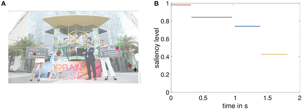
Figure 3. An example of the fixation data sequence in one trial. (A) Shows five fixation locations overlaid on the original image and their numerical order (the numbers are labeled in green). The radius of the red circle indicates the duration of each fixation. (B) Plots the saliency levels of the fixations in (A) against the corresponding timestamp in that trial. Salience is normalized from 0 to 1 within an image. This specific trial starts at time zero. Note that the third fixation is extremely short and hence is barely visible; it is plotted as a dot with saliency near one.

Figure 3B shows the same data in a time series, which also plots (on the y-axis) the SAM-model salience of the location at which the eye happened to be fixated at the time on the x-axis. In this example, the fixations happen to be a step function that decreases in salience from high to low (except for the super-short fixation 3). That is not true in all trials, as the HMM will show. As is well-known in human visual perception, it is evident in this example that the eye is performing a series of rapid, discrete fixations (generally about 200–300 ms long), transitioning rapidly between fixations.

With this example in mind, we now explain how salience judgments are made. Bottom-up salience is a concept from cognitive psychology and neuroscience. Visual features that are bottom-up are low-level features, such as color, orientation, intensity (brightness), centrality, and high-level features such as objects, faces, or animals. Top-down salience is the features of an image that a viewer will direct attention to achieve a goal (e.g., maximize a rationally-inattentive objective function). It is well-established that people tend to look at bottom-up salient locations in the first 3–5 s of passive viewing, and that algorithms can predict where they look quite accurately (see Li and Camerer, 2022 for background details).

The algorithm we use is a “deep learning” convolutional neural net trained on several “free viewing” data sets to compute bottom-up salience for all image locations (Cornia et al., 2018). The data came from several hundred people looking at large sets of natural images of different kinds for 3–5 s, without any special goal in mind. Their eye fixations were recorded with a physical eye-tracker or a software-implemented pseudo-eye-tracker. The networks are trained to predict accurately where most players look.

For the simplest discrete HMM, called dHMM, we observe the order of fixations but not their duration. It is reasonable to approximate the dynamic continuous attentional process as a series of discrete transitions between states corresponding to different levels of salience, ignoring the duration difference for new fixations.¹⁰

As noted previously, the HMM hypothesizes four states: start state S, decision state D, and two L and H salience hidden states. While other assumptions about the number of hidden states were tried, we found that two hidden states give the optimal BIC value (see Appendix for details). One can specify more different hidden states like three, four, or more salience-level states. But the best-fitted results indicate that people do not distinguish any finer scale of saliency other than the H and L levels when they are playing these games. This is an interesting finding on its own. There is no theory or intuition about why there are only two saliency states. It is possible that players simply categorize saliency states crudely into high and low (which is especially useful for the hider-seeker game). It may also be that we do not have enough data, or trials with long enough sequences of fixations, to detect more states. Studies explicitly designed to figure out different possible structures would therefore be useful.

The parameters that need to be estimated from the eye-tracking data are the transition probability matrix P, and the means and variances of the Gaussian L and H salience distributions. The starting state has two transition probabilities, p(L∣S) and p(H∣S), as well as a rare transition p(D∣S).¹¹

The states L and H self-transition internally with probabilities P(L∣L) and P(H∣H), and transition between each other with probabilities P(L∣H) and P(H∣L), and eventually transition to D with probabilities P(D∣L) and P(D∣H). As noted, the estimation is done using the standard Baum-Welch algorithm through the HMM estimation toolbox in Matlab (Murphy, 1998; see Appendix for details).

Figure 4 shows a graphic display of estimated transition probabilities between states, and the estimated Gaussian distributions of salience in the L and H states. There are three figures, each corresponding to matching, hiding, and seeking.

FIGURE 4

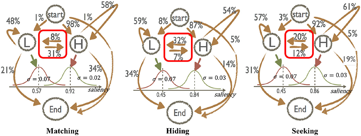
Figure 4. This figure shows the estimated HMM for three different games, matching, hiding and seeking, separately. The estimated parameters consist of two parts: The matrix P that gives the probabilities of being at the hidden states, and the parameters of Gaussian transition processes, which connect the hidden variables and the gaze observables. In example in the hiding transition figure you can see that the probability of the next fixation being in a high saliency (H) state given that you are currently in a H state is 54% and that the probability of switching to the low saliency (L) state is 32%. Likewise the probability of switching to a H state given you are in an L state is 7% and that the probability that you switch to another L state is 59%.

In all three games, subjects transition from Start S to State H most often (over 90% of the time). These high values of P(H∣S) in all games is evidence that SAM, which was trained on free gazes of other people to predict the saliency of an image, not on games, is doing a good job predicting where the game-playing subjects look initially. The fixation transitions afterward vary by the game structure and the subject's strategic role.

Transitions to the decision node D are also different across games. In matching games, conditional transitions to D from H states are more common than from L states (34 vs. 21%). In matching games transitions from L to H are more common (31%) than transitions from H to L (8%).

Readers who are new to HMM can think of these diagrams as simply reporting a lot of conditional probabilities which are interesting. For example, one interesting question is the conditional probabilities P(H∣Start), P(L∣start) for hiders and seekers. These conditional probabilities allow us to ask the question of whether hiders and seekers begin their games differently. The answer is basically No; 87% of hiders and 92% of seekers start at the high-saliency H state. These data imply that even though their top-down attentional goal is to find low-saliency locations, hiders automatically look at high-saliency locations first (87% of the time). There are lots of other questions about conditional probability that are behaviorally interesting. The HMM gives all of these answers. And instead of computing such statistics in a piecemeal fashion, the conditional probabilities are all forced to come together into a constrained and coherent whole.

In hider-seeker games, the transition rates among low- and high-salience L and H states are different for hiders and seekers. Hiders have a large asymmetry in rates of transitioning from H to L (32%) compared to L to H (7%); this shows that these players are looking for inconspicuous (low-salience) places to hide. Seekers exhibit a similar difference but the asymmetry is smaller (21% and 12%). Hiders are slightly more likely to transition out of salient H states (instead of L states) to D (14%) compared to seekers (18%), reflecting strategic thinking by the hiders.

The estimated L and H state Gaussian saliency distribution means are rather close across all three structures: The means are (0.57, 0.90) in matching, and (0.45, 0.84) and (0.45, 0.86) for hiders and seekers, respectively. Recall that every image contains many low-salience locations because saliency values are normalized to range from 0 to 1 in each image. However, the estimated Gaussian means of saliency in states L and H are around 0.50 and 0.90, respectively. This implies that deeply low-salience locations (saliency levels below 0.40) are fixated on so rarely that the model practically ignores them. This is an important insight because it indicates that hiders have limited strategic thinking (or a limited perceptual inability to find very low-salience locations) which explains the seeker's advantage in winning more often than predicted by Nash equilibrium.

5. A new way to identify strategic thinking levels

This section introduces a new way to identify levels of strategic thinking based on HMM transition data. The method relies on a simple assumption: when people are reasoning between different strategic options, their eye movements are associated with thinking. Under this assumption, we hypothesize that in hider-seeker games higher-level players transition back and forth between different H and L states more often, and low-level players have fewer fixations and transitions, and faster response times. The HMM method can then be used to infer an estimated k level on a single trial basis (based on the number of state transitions), given a game structure and gaze data. We will illustrate how it works in these location games.

Level estimations can be sensitive to the specification of what level 0 players do. The HMM solves this problem by using the data to infer initial state probabilities (assuming the starting state is the level 0 choice, which is as plausible as any other conventional assumption). Second, in many games, such as 2 × 2 normal-form games with mixed equilibria and some games with strategic substitution, predicted choices cycle in the sense that the same choice can be made by players using both low and high levels of reasoning.¹² While some elegantly designed games have been created that do not predict level-k cycling and hence make level classification easier (including the 11–20 money request game, p-beauty contest game, and ring games Nagel, 1995; Arad and Rubinstein, 2012; Lindner and Sutter, 2013; Kneeland, 2015). However, many games of economic interest will have classification challenges.

Given an estimated HMM model $\widehat{ℍ}$, suppose a vector of fixation emissions denoted by f = [f₁, f₂, ..f_m] is observed in a single trial under game G. The vector f can be projected back to h, so that we get an ordered vector in the estimated hidden state space by maximizing the posterior probability: $P(h_t\mid \text{f},\widehat{ℍ},h_{t-1})$ sequentially. Formally, a projection function g_{o → ω}: O → Ω is defined as:

$g_{o\to \omega }(\text{f})={\displaystyle \underset{\text{h}}{argmax}}P(\text{f}\mid \text{h},\widehat{ℍ})$

Thus, the fixation vectors are now all transformed into hidden state vectors. Take the salience game Hider as an example. A recovered hidden state transition vector from actual fixations might be [S, L, H, H, H, D].

With this transformed data set, strategic thinking levels can be defined based on inferred hidden state transitions. First, we assume that the initial fixation is the level 0 response as several other studies have shown evidence that level 0 choices are more likely to be salient options (e.g., Crawford and Iriberri, 2007a).¹³

Then we further assume that players switch roles when they are trying to mentally simulate other players' moves. Each directional transition that fits the best response function of game G and a current simulated level s and role $\widehat{i_t}$ adds one more level. And just like the textbook best response notation $b_{\widehat{i_t}}({\sigma }_{\widehat{i_{t-1}}})$, the best response function maps to a set of strategies of the current player $\widehat{i_t}$ when her hypothetical opponent (given by her last stage thought) chooses ${\sigma }_{\widehat{i_{t-1}}}$. For instance, one's best response is to choose the most salient location if she wants to coordinate. An estimated level using HMM will be the sum of all such switches in levels. For example, a transition vector [L, L, H, L, L, D] in hider-seeker games will be identified as level 2 because there is a transition from L to H and then from H to L.

Formally, given a transition vector h = {h₁, h₂...h_t...} in a single trial and the best-response function B of the game, the strategic level is defined by:

$\text{k}={\displaystyle \sum _t}11({\sigma }_{\widehat{i_t}}=\text{B}({\sigma }_{\widehat{i_{t-1}}}))$

With fixation transition emissions and an estimated HMM model based on those fixations, the above procedure can estimate a system of strategic levels on a single-choice basis (one level for each choice). Figure 5 shows the estimated level distributions of three different games aggregated for all subjects and all images.¹⁴

FIGURE 5

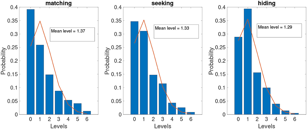
Figure 5. Level identification from gaze transitions and HMM. The blue bar shows the histogram of levels identified using the gaze transition method using all gaze data across all individuals. The red line is the best-fit Poisson distribution of the gaze-identified level distribution.

These level identification results show an approximately exponential decline but also fit reasonably well to a Poisson distribution, which is consistent with the simplifying assumption made in the Poisson cognitive hierarchy model. The best-fitted τs are 1.37, 1.33, and 1.29 for matching, seeking, and hiding, respectively.

Note that the estimated frequency of level-0 types for both seeking and hiding is high; it is around 30%. However, these frequencies are roughly consistent with the Poisson specification with low values of τs (1.33, 1.29). And note that the Poisson frequencies for level 1 and above match quite closely (i.e., the Poisson distribution is a good fit for the estimation of level types from the HMM).

In matching games, the level-0 frequency is estimated to be quite high, at around 40%. But remember in the matching games the goal is to find a location that will match what others will see. Finding a highly salient location can end the strategic process—and often, it should end the process. Indeed, this result is likely to be consistent with what is predicted by a model in which levels are endogenously chosen based on the assessed benefit of thinking further. In matching games, if a salient choice is made that is likely to match, there is little benefit to looking further Alaoui and Penta (2016) so it is endogenously optimal to stop at level 0. In our matching games there are range of images with high and low density of saliency centers CONOR.

Similar to many previous estimates, the HMM level identification indicates that most specific-trial inferred levels are below k = 3. This is a non-obvious result because eye saccades are effortless; a highly strategic hider, for example, could easily transition back and forth from L to H states three or more times in a few seconds. Yet our study finds that players who make three or more transitions are rare.

Figure 6 compares the mean of population levels¹⁵ by using our gaze-predicted method and two previous methods: structural cognitive hierarchy and level-k models (for details about these two benchmark models, see Li and Camerer, 2022). As can be seen, the estimated mean level of the new method lies between the mean level from the cognitive hierarchy model and the level-k model. Furthermore, using our new method, the strategic level in hiding games is not different from that in seeking games (p = 0.24), while in matching games, people behave as lower types than in the hider-seeker game (p < 10⁻⁴).

FIGURE 6

Figure 6. Comparison of levels between the gaze estimated method and benchmark traditional methods. The blue bars are the average levels estimated using gaze data. Red bars are those levels using cognitive hierarchy method. Yellow bars are the levels using level-k method (assuming level-k players best response to k-1 group). The level-k model suffers from an identification issue in matching games, the choice prediction is exactly the same for all levels, therefore, the yellow bar is omitted there.

Note that this level classification is done on a single-trial basis. Each subject has a level classification for each trial and game type. We can therefore explore how consistent players are in their level of strategic thinking across roles and games. The estimated individual-game base levels are shown in Figure 7. One dot indicates the average strategic level for one person and one game. We found that individuals' levels are correlated for separate hiding games and seeking game estimations as can be roughly seen in the figure (that is most of the yellow and orange dots are close to one another, and the correlation coefficient for hider- and seeker-levels is ρ = 0.55, p = 0.005). However, in the matching game players' levels are often quite different from those in hider-seeker games (no significant correlation was found). This result suggests that individuals behave rather consistently in similar level depths when they encounter similar strategic situations. It could be useful to test the individual consistency in a wider range of games in the future to see how different/same people behave under different strategic categories.

FIGURE 7

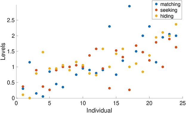
Figure 7. Estimated strategic levels across games at individual level. Each dot shows the average strategic level of one individual in one game session. Three dots in one column represents levels of different games for one individual. We order the data of all individuals by their mean level performance (average of the three dots), from low to high going left to right.

Because we have limited data per subject, the HMM analyses aggregated data across subjects to give only a general picture of the nature and frequency of high- and low-salience transitions (that's in Figure 4). Thoughtful readers have asked about what might be learned about other types of likely behavior from our eye-tracking data and from the HMM that distills all those data into states and transitions.

• Wouldn't the initial search phase likely exhibit some transitions between an H and L state at least once? The answer is that as the HMM transition rates show, this type of automatic high-to-low exploration behavior is not all that common. When in the high-salience state, hiders and seekers transition out with probability 0.32 and 0.21. Keep in mind that subjects have six seconds to choose, and each image is unique.

• How would we expect random or clueless players to behave? This is an important question. In experimental economics, we usually think of “clueless” (or unmotivated, or tired) subjects as choosing randomly and quickly. But in these experiments, truly choosing randomly among pixels means ignoring their visual salience. A huge amount of evolved adaptation and dedicated neural circuitry is devoted, in the human brain (and in other mammals) to responding to salience. So “clueless” players are unlikely to look at all aspects of an image-they are more likely to look at high-salience locations automatically and not look much more. That is precisely why we estimate a substantial percentage of level-0 thinkers given the HMM results.

• Do multiple transitions between L and H states necessarily show higher sophistication? Perhaps players are just “making sure” of the relative salience by comparing the two states again. Our answer to this question is that salience is a rapidly-coded property of a location. It is not like a number in a payoff matrix, which a person may need to keep in mind as part of a working memory-constrained calculation (like finding the level-1 strategy), and might therefore re-fixate on to improve memory. It is, of course, conceivable that players transition from H to L to H, but when they do it will be coded (perhaps “over coded”) as high-level behavior, and as is evident in Figure 5, such multiple transitions are rare.

• How confident should we be about the inferred levels of reasoning in Figure 5? The answer is that there are certainly many strong assumptions that go into inferring these levels from the H-to-L transitions so we cannot be very confident. But we are confident that the eye-tracking data, as distilled into an HMM, is an improvement over trying to infer level-k and cognitive hierarchy model parameters purely from choices. In Li and Camerer (2022), the cognitive hierarchy just seems wrong. The problem is that higher-level hiders should choose low-salience locations and they just do not make those choices very often. The model is so rigid that it has no choice but to infer a low average level τ. Level-k models are more flexible about the frequencies of level types and deliver frequencies more similar to many other studies, but the overall fit is only a little better for level k. In our view, using the H-to-L salience transitions is a better biomarker of plausible level-k transitions than the inference in Li and Camerer (2022) which did not use eye-tracking data.

6. Using a continuous-time cHMM

The discrete dHMM model can be further extended to a continuous Hidden Markov Model (cHMM) to predict choices under time pressure. The cHMM preserves all the properties of the discrete HMM, but it also adds information about the time length of fixations.

A cHMM inherits everything from dHMM except that the probability of transitioning to state j from i at time t is redefined with respect to time denoted by P_ij(t). In Section 3.2, we already estimated the transition probability matrix $\widehat{P}$ and $\widehat{\mu }$. In this section, the main goal is to estimate P_ij(t), the dynamic profile of time-stamped transition probabilities over time.

This addition enables cHMM to predict how long the decision-maker will stay in each hidden state and the probability of observing a particular data emission at each time point beginning from time zero. A sample prediction would be: at time 2 s when the decision-maker is in a hidden state (L), she will switch to another hidden state H with a probability of 0.7.

The cHMM model makes predictions about what information a decision-maker will look at, and which strategy they will choose if the exogenous limit on response time is reached. Specifically, a cHMM can answer the following question: If the dynamic strategic process of the player is artificially truncated earlier, what does the player do? Does she not have time to find a reasonable strategy, and hence suffers from losing more in the game under time pressure?

Next, we will use data from the salience game to validate the prediction. Similar to the previous section, the association function is assumed to be Gaussian, thus the model is called the continuous-time Gaussian Hidden Markov Model (cHMM). As in dHMM, the data set consists of emission vectors, which are the saliency values of the fixation location. In cHMM, the saliency values of these fixations are combined with the duration of eye fixation at the location of interest. As with the estimated dHMM model, we use the standard MLE method described in Ross (2002) and a cHMM package tutorial¹⁶ to further estimate P_ij(t) for each game. The results of estimated salience levels output by the continuous models are shown in Figure 8. The model predicts that in all three games, people start at salient locations (H) in the first couple of hundred milliseconds. In the matching game, the decision path mostly stays in state H and so the predicted saliency level falls only slightly over time. In hider-seeker games, the probability of being at the high-saliency state H drops much faster than in the matching game and drops more rapidly for hiders than for seekers.

FIGURE 8

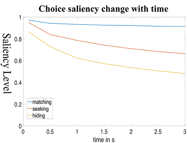
Figure 8. cHMM model predictions of salience strategy over time. The figure shows the probability of people being in the high-salience state as time goes by in the unit of seconds. The simulation results of cHMM predicting the matching rate averaged against reaction time over all the task images. Point X is the estimated average matching rate of the time-pressure group and point Y is the estimated average matching rate of the baseline (no time pressure) group.

The basic prediction is that time pressure will increase the average saliency of locations chosen because over time the general trend of both seekers and—more strongly—hiders will be to transition from H to L during a trial. If that process is interrupted prematurely, average salience levels will be higher as the player will not have time to shift their fixations to lower salient locations. That should lead to increased matching rates, and thus seekers will win more often. Time pressure should therefore increase the seeker's advantage.

That directional prediction is not too surprising. However, the goal here is more ambitious than just predicting the direction of the effect. The HMM predicts the numerical size of the seeker's advantage for various amounts of time pressure. Note that a crucial maintained assumption in this exercise is that players do not adjust their HMM structure due to time pressure. If this assumption is wrong, the predicted effects of time pressure will not be accurate.

To test this hypothesis, we compared two new groups from mTurk. The control group (N = 38) faced the same experimental setting as the lab subjects (with a constraint of 6 s for response). The treatment group (N = 31) had a shorter time constraint of 2 s. All other features of the design were unchanged.¹⁷

The seeker's advantage between control (time limit = 6 s) and time-pressure treatment groups (time limit = 2 s) was measured in new experimental sessions.¹⁸ In the baseline 6 s condition, the online group still shows a significant seeker's advantage at precisely the same matching rate, 0.09, as in the local lab population. The seeker's win rate increased significantly to 0.15 (p < 10⁻⁴, t-test) in the time pressure condition. This result is shown in Figure 9, labeled by point X (time-pressure matching rate) and point Y (baseline matching rate). The cHMM model correctly predicts the change in seeker win rate will go up from 6 s to 2 s deadlines, although the predicted magnitude of change is only about half as large as the change in the actual data.

FIGURE 9

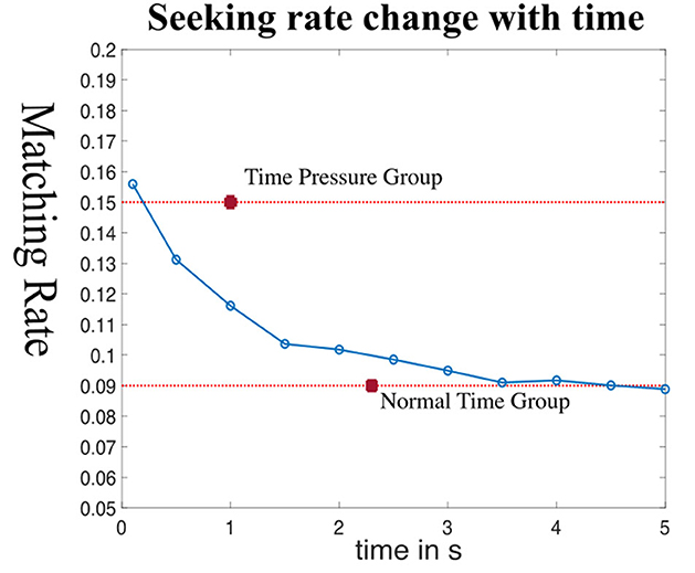
Figure 9. cHMM model rate change over time. Simulation results of cHMM which predict the matching rate against reaction time over all the task images. Point Time Pressure Group is the estimated average matching rate of the time-pressure group and point Normal Time Group is the estimated average matching rate of the baseline (no time pressure) group. Finally note that time-pressure should not change the matching rate in matching games, because the saliency change is very little.

To investigate whether this increase in the seeker's advantage was due to subjects choosing more salient locations under time pressure, we compared the mean saliency level of location choices in the control and time pressure treatments. Hiders' mean choice saliency increased under time pressure, from 0.52 to 0.59. The corresponding seekers' mean saliency rose from 0.61 to 0.81.

Note that in the no-feedback condition, the seeker win rate was a bit higher than the feedback condition, 0.23 (We do not have a particularly clever explanation for why this rate is higher than the 0.15 observed for feedback, except that opportunities to learn from feedback decrease noise.).

Thus, our understanding of how saliency interacts with the depth of strategic thinking enabled us to predict a change in seeker advantage due to time pressure. While the effect of time pressure might seem obvious, no model currently used in behavioral game theory predicts this change.¹⁹ That is because there are no theories integrating salience and dynamic attention as the HMMs do. The prediction that the seeker's win rate will go up under time pressure is indeed intuitive, but it rests entirely on the hypothesis that under time pressure, hiders cannot inhibit the automatic tendency to look at—and also choose—salient locations. Additionally, the cHMM goes even further than that time pressure intuition by delivering a continuous predicted profile of seeker win rates across the entire range of game durations. It should be easy to imagine interesting experiments testing such numerical predictions on these data and many others where dynamic attention is measured and understood.

An important methodological comment is that in economics experiments it is not generally thought to be likely, or even important, that exact numerical results generalize from lab to field. There is typically sufficient difference between a simple artificial lab environment and a target field setting (to which there is intended generalizability) that we do not expect specific numerical results to carry over from the lab to the field. For example, how much lab workers reciprocate being paid generous “gift exchange” wages, in numerical terms, is unlikely to give a good estimate of workers in a company reciprocating year-end bonuses with extra January work hours. The exact number derived from the simpler lab environment is not designed to be a number useful in predicting company bonus reactions. In those common cases, the lab is thought to be useful for generating qualitative insights—such as the sign of an effect, and whether it is small or large (compared to prior beliefs or other studies). It is not expected to generate portable quantitative insights (see Kessler and Vesterlund, 2015 for a good articulation of this view).

The importance of the precision of the cHMM-derived time pressure prediction here is different. In our case, the precision shows that when a method such as dynamic HMM is applied to one set of decisions, and a prediction is derived from interrupting the HMM, the prediction is precise and not too far off. This suggests that if an HMM was used to study states in field data (as has been done in macroeconomics), and the HMM is interrupted in a certain way, the prediction based on interruption would not be too far off either. The numbers would of course be different, but the ability of the interrupted-HMM procedure to produce a reasonably accurate prediction is—we conjecture—likely to have some accuracy.

7. Discussion

In this paper, HMMs were used to distill eye-tracking data to understand strategic dynamics in visual location games. The HMM derives the best way to infer hidden states and connect them to observable eye fixations and strategic choices. The best-fitting model shows that players generally begin trials by fixating on highly salient choice locations, regardless of game structures. Transitions to high- and low-salience states then take place at different rates depending on the goal in each; matching, hiding, or seeking.

The HMM itself is novel and is hopefully an insightful way to summarize the cognitive process and compare it across player roles. Beyond those insights, HMM is used to generate two new insights.

The first insight is how to estimate level-k models. We created a new method to classify the strategic thinking level for every game trial using the trained HMM. The results consolidate previous findings that level frequencies are often approximated by a Poisson distribution, and the average level is around 1.5. The new type classification has two differences (and potential advantages) over previous methods: (1) Level identification does not depend on an a priori level 0 specification; and (2) levels are defined by inferred state transitions.²⁰ The resulting level profiles—with average levels around 1.3—match other experimental data sets reasonably well.

The second insight uses continuous-time cHMM built on top of the dHMM. dHMM is a model of discrete state transitions but does not have a running time clock– it runs on event sequences, not clock time.²¹ The continuous model includes the fixation time lengths and uses them to predict a time profile of salience level choices. This model successfully predicts a change in matching rates in hider-seeker games when there is exogenous time pressure, although it does under-predict the magnitude of the effect.

Additionally, we believe that our findings can be extended to non-location-based games. There is evidence to suggest that the same saliency algorithm we used in our location games can be used effectively to discern saliency in other domains such as identifying salient locations of a stock chart (Bose et al., 2020) or in a matrix game (Li and Camerer, 2022). With this knowledge, we believe our HMM approach can be extended to gain insight into the reasoning of players in these games as well.

One limitation of our study—and all other studies measuring time and visual fixation—is that we do not know exactly how people are reasoning about the game independently of their visual fixations. The presumption in HMM using fixations is that fixations are reflecting a choice process. The working assumption is that when a payoff or structural feature is not seen it is not used in computation. This assumption may underestimate strategic thinking levels because it does not identify higher-level players who are reasoning mentally (e.g., using memory) without redirecting their gaze. We suspect that such reasoning-without-seeing behavior will be less prevalent when the game is novel or complicated.

An important open question for behavioral game theory is whether the HMM method might help address the challenge of portability, raised most sharply by Hargreaves Heap et al. (2014). Portability in general is the ability to predict from model parameter estimates in one game to other games, preferably new games that are different in structure.²² [Hargreaves Heap et al. (2014) are skeptical about portability of level-k models. Crawford (2014) challenges their skepticism.] One type of useful portability is how trait-like level-k thinking levels are, for an individual, across different types of games. In psychology, this long-standing question is called “states versus traits.”

Deriving thinking levels from an HMM or some other dimension-reduced use of fixations and choices can address the problem of personal-parameter portability (i.e., traits) to some extent, but not directly. Since HMM levels are defined on single trials instead of people, it naturally relaxes the condition that the same individual should necessarily have consistent thinking levels across games (Indeed, analyses like Alaoui and Penta, 2016 which endogenize thinking suggest levels should not be the same across games, or even in different games within a person, because endogenous levels will depend on payoff incentives for more thinking.). It is still meaningful, though, to ask this question: do people have different abilities in strategic games? If so, how should we define ability? A possible future research direction is to collect large data sets across subjects on different games, making sure to collect their gaze data, and then to use HMMs to investigate the differences in depth of strategic thinking across people and game structures.

Note that HMMs have even more general applications than the ones used here. Any observable information can be used as covariates, to estimate the state transition matrix P or condition its values. For example, if the trial number t is included, the HMM can estimate whether learning—in the form of changes in transition rates based on t—is happening over the course of an experiment.

Many social scientists outside of psychology are now drawn to, and trying to make sense of, the idea and value of a dual-process “system 1, system 2” type of decision-making (Kahneman, 2003, 2011). This idea originated in studies of the psychology of judgment. If there really are two dissociable systems of perception and judgment, and they transition sequentially from system 1 to system 2, a two-state HMM is ideally suited to identifying the states and their properties and transition rates.

HMMs may be applied insightfully in other domains of experimental economics besides matching and competitive hider-seeker games. Any domain in which data or theory suggest there might be distinct modes in a mixture distribution of observables, and in which those modes are stochastically related to hidden hypothesized states, is a good candidate for HMM analysis. These could be the mental states of individuals fixating on locations in visual images, in our location games, or collective or individual states in auctions or markets. Here are some speculative examples:

• Market equilibrium: Classroom supply-demand experiments study equilibration and efficiency in markets for perishable goods (see Smith, 1962; Lin et al., 2020). The observables are the timing of bid and ask arrivals and the resulting “order book,” price levels and changes, etc. Plausible hidden states are whether the market is near competitive equilibrium or not.

• Bubbles: The observables are features of price changes, bid and ask arrivals, and the resulting “order book,” social media discussion (Shiller, 2015, 2020, or even brain activity of traders, Smith et al., 2014). Plausible hidden states are whether a stock is in a price bubble.

• Optimal bidding: Experimental bidders in second-price Vickrey auctions do not always bid their values (though it is a dominant strategy to do so). The observables are bids, response times, and even neural activity measured by fMRI (Grether et al., 2007). Plausible hidden states are bidding in and out of equilibrium. Related applications include: “Game form recognition” (Chou et al., 2009; Cason and Plott, 2014; Bull et al., 2016) and “epiphany” learning where a player seems to suddenly discover an optimal strategy (Chen and Krajbich, 2017; Chen and Wang, 2020) (Those models might be a lot like how regime shifts are studied using HMMs in macroeconomics—an epiphany is a mental regime shift.).

  A more general question is whether bidders adjust bidding rules dynamically. Others applied an HMM to experimental data from English and first-price sealed-bid auctions (Shachat and Wei, 2012). They find a slight tendency to shift from best response bidding to an absolute markup (fixed profit) rule.

• Deception in sender-receiver games: The observables are timing and content of sender messages and receiver actions, and potentially eye-tracking, pupil dilation, psychophysiology, facial muscles, etc. (Crawford and Sobel, 1982; Wang et al., 2010). Plausible hidden states are whether senders are deceptive and whether receivers are naïve or sophisticated. Other experimental paradigms in which there may be deception and lying (Abeler et al., 2019) could be studied similarly using HMM. A related application is detecting collusive states in experimental markets (Fonseca and Normann, 2008).

• Insider trading: A challenge for securities regulators is detecting whether insiders are illegally trading in a market (Detecting market manipulation is a similar challenge conceptually.). The observables are features of bid and ask arrivals and the resulting order book, block size and trader identity of orders, etc. Plausible hidden states are whether insiders are trading in the market. An advantage of using lab experiments is that one can control the number of insiders. A derived HMM that tries to infer insider trading can then be matched with the actual insider trading observed in the experiment.

• Cooling off: In ultimatum games, it is well-established that many responders reject positive offers of money (see Lin et al., 2020 for recent evidence). Rejections appear to reflect a trade-off between receiving money and tolerating unfair inequality. A related interpretation is that the rejection decision is influenced by an emotion such as anger at being treated unfairly. If so, the emotion might be transitory so that an angry respondent “cools off” over time, and is more likely to accept the same offer if she has to wait a while. There is mixed evidence that waiting periods can affect rejection rates (although in both directions, Cardella and Chiu, 2012; Oechssler et al., 2015). In this example, possible observables are emotion measures (e.g., facial emotion see Nguyen and Noussair, 2014), arousal such as galvanic skin response, self-reported emotions, etc. Plausible hidden states are whether the respondent is in the “hot” emotional state or has cooled off. By varying the length of time between receiving an offer and responding, HMM could deliver a prediction about roughly when the cooling-off occurs.

We add two remarks about the speculative examples that were just listed: First, in most previous research on these topics the experimenters use a specialized statistical analysis which essentially tries to associate observables with hidden states, without using the language of HMM. For example, in a single-period supply-demand experiment, measures such as how much prices deviate from a predicted competitive equilibrium crudely distinguish whether the market is in equilibrium or not.

In HMM those two states—the market in and out of equilibrium—would be treated as hidden states which are hypothesized to be statistically identifiable by observable “emissions.” The key difference is that HMM is appropriate, and is likely to add insight when observables appear to be created by a mixture of statistical modes. For example, in the equilibrium hidden state, the trade-to-trade price changes might be much smaller in magnitude than when in the out-of-equilibrium state. That is, a histogram of price changes would look like a non-Gaussian mixture of a big spike at price changes close to zero, in equilibrium, and another variable distribution with larger changes which is out-of-equilibrium adjustment. Because cHMM is dynamic, it could also provide a tentative answer to the question: When did the market reach equilibrium?²³ The answer would be the time at which the market is in the “equilibrium” state with high probability and is unlikely to transition out of that state. There might also be more than two states which represent various degrees of near-equilibration.

Second, in many cases, the important behavioral states are not hidden and are known to the experimenter. For example, in a sender-receiver game, an experimenter can directly measure if a sender is deceptive by comparing the sender's message and the true state because the true state is known to the experimenter. What is “hidden” is the observable aspects of activity—mouse movements, perhaps eyetracking or facial emotion– which are associated with what an experimenter knows is a deceptive behavior. Then one could train an HMM using those other kinds of data (and knowing whether a sender is deceptive or not), then use it as a generative model to infer a true state that is known to the sender but not to the experimenter. Such a model could conceivably be applied to data in a field application outside the lab where true states are unknown. For example, an HMM could be trained to detect whether bidding is in equilibrium in a setting where the experimenter knows the bidders' true object values, then use it in an experiment or field setting to detect whether bidders appear to be bidding in equilibrium or not.

Finally, putting aside the HMM framework, this paper adds to evidence from Li and Camerer (2022) about the potential value of algorithmic measures of visual salience to study decision making and economics. In simple decisions with mild time pressure, bottom-up attention based on the salience SAM is designed precisely to predict a lot of what people first notice, which will often influence decisions. In retail stores, vendors pay a premium for shelf space at eye-level because products at that location are central in the visual field and are therefore more rapidly salient. “Nudges” make simple changes to choice architecture that impose low costs, and improve decisions as consumers or citizens themselves would judge them. For many such decisions, making desirable choices more visually salient is something that is not difficult to do, using algorithms such as SAM (or a more locally-tuned algorithm) but is not a large, systematic part of current nudge cartography.

Data availability statement

The original contributions presented in the study are included in the article/Supplementary material, further inquiries can be directed to the corresponding author.

Ethics statement

The studies involving human participants were reviewed and approved by Institutional Review Board at Caltech. The patients/participants provided their written informed consent to participate in this study.

Author contributions

XL and CC contributed to the conception and design of the study. XL conducted experiments, performed the statistical analysis, and wrote the first draft of the manuscript. All authors contributed to the manuscript revision, read, and approved the submitted version.

Funding

The study was supported by the Behavioral and Neuroeconomics Discovery Fund (PI CC), Tianqiao and Chrissy Chen Center for Social and Decision Neuroscience (XL and TH), Alfred P. Sloan Foundation (G201811259), and NIMH Conte Center P50MH094258.

Acknowledgments

Thanks to audiences at the Society for Neuroeconomics.

Conflict of interest

The authors declare that the research was conducted in the absence of any commercial or financial relationships that could be construed as a potential conflict of interest.

The author CC declared that they were an editorial board member of Frontiers at the time of submission. This had no impact on the peer review process and the final decision.

Publisher's note

All claims expressed in this article are solely those of the authors and do not necessarily represent those of their affiliated organizations, or those of the publisher, the editors and the reviewers. Any product that may be evaluated in this article, or claim that may be made by its manufacturer, is not guaranteed or endorsed by the publisher.

Supplementary material

The Supplementary Material for this article can be found online at: https://www.frontiersin.org/articles/10.3389/frbhe.2023.1225856/full#supplementary-material

Footnotes

1. ^Connection to finite state “machines” were in vogue in the 1980–1990s in game theory. The main idea is to find the strategy transitioning pattern during repeated games using automata structures, which share some similarities with HMM. Both of them contain state-transitioning structures. Abreu and Rubinstein (1988) analyzes equilibrium using two-person repeated games with automata and shows interesting findings on equilibrium selection. Almanasra et al. (2013) studies different types of automata like adaptive or cellular. Unlike automata games, which are in the repeated game regime, HMM studies the process of one-shot games.

2. ^For example, suppose we could read the eyes and mind of a chess player perfectly as she plans a move from a current board position B_t. The board position is a plausible state. Transitions to new board positions B_t+1 correspond to moving a chess piece. A plausible model of her process of “playing” is that she is mentally simulating different sequences of transitions from the current board-position state to different future board-position states. But as she is playing, her mental process of imagining probabilistic transition is hidden from us.

3. ^SAM is an Attentive Convolutional Long Short-Term Memory network (Attentive ConvLSTM) model which can predict human eye fixations on natural images.

4. ^Brocas et al. (2014) reported distributions of lookup times in different normal-form game payoff cells. However, they are highly correlated with lookup frequency (since the time per lookup usually has low variance) and they did not use timing data in a sophisticated way to infer decision rules.

5. ^Generative models are compared with discriminative models. The latter is used to distinguish different classes while the former can be used to generate new data. HMM is a typical generative model.

6. ^The time-interrupted predictions can also be compared to the experimental “always be choosing” protocol used by Agranov et al. (2015). In that protocol, subjects are continuously expressing a choice (e.g., using a slider bar or mouse) and there is a probability that the recorded choice at any time point will be randomly chosen for payment.

7. ^In Li and Camerer (2022), the game data were used to estimate level-k models using only choices. The eye-tracking data were not used in the main text. That paper also includes two other data sets. The HMM analysis using eye-tracking as observations reported here is new, as are the level-k identification and effect of time pressure.

8. ^If the pixel-centered circle extends outside the 2D boundary, the out-of-bounds portion wraps around to the opposite side, as if the 2D image is a torus.

9. ^Li and Camerer (2022) also did an experimental treatment in which the circle size is 1.5 times bigger, and the predicting matching rate in the hider-seeker game is 16% instead of 7.1%. The difference between the seeker win rate and the Nash predicted win rate is +2%, the same as in the baseline condition.

10. ^Some readers will be familiar with dynamic process models which hypothesize a hidden accumulator or “drift-diffusion” models (DDM) leading to choice (Ratcliff and McKoon, 2008; Ratcliff et al., 2016). These models are designed to explain choices, error rates, response times (RTs), and differential RTs for correct and erroneous choices (Krajbich et al., 2010; Ratcliff et al., 2016; Fudenberg, 2020). DDM models are not ideal because, as Figures 3A, B indicate, the core mental process is the transitions between salience levels rather than accumulation toward one of two boundaries. It would certainly be useful in future research to compare DDM and HMM more carefully.

11. ^These transitions from S directly to D only happened 1% of the time in matching and 5% in hider-seeker games. And they are caused by a few players who made their choices without even one fixation. The low probability of these transitions also provides additional evidence that most people, even after many trials, do make decisions by looking at the stimulus.

12. ^That is, there exist strategies s_i, s.t s_i∈B_i[B_−ℶ(s_i)].

13. ^An open topic in behavioral game theory is the ideal cross-game specification of level 0 player choices. Early versions assumed level 0's randomized across all strategies. Our current thinking is that level-0 players choose salient strategies; equal randomization as a default when strategies are equally salient. This assumption obviously begs the question of what makes strategies salient to level 0's. In location games, visual salience is one answer, and the HMM estimate that P(L∣S) is around 0.90 is strong evidence for this answer. Other papers with large numbers as strategies have also found concentration on ”lucky numbers”—e.g., Ho et al. (1998) found a large number of Singaporean subjects choose 80 or 88 in the p-beauty contest game (because 8 is a lucky number for many Chinese). In a Swedish lottery game, LUPI choosing numbers from one to five digits, Östling et al. (2011) found that disproportionately many people picked numbers corresponding to birth years (e.g., 1900–2000). In games with private information states, both auctions and sender-receiver games, it appears that level-0 players choose strategies equal to their private information. For example a level 0 player with a private value V bids that same number in an auction, and a level 0 sender's message is the true state (Cai and Wang, 2006; Crawford and Iriberri, 2007b; Wang et al., 2010).

14. ^One reviewer asked whether there are more H or L locations and hence, whether there could be more opportunities for transitions from one state to the other. The saliency values in an image are always normalized so they are uniformly distributed from 0 to 1. In the H and L states as estimated, the standard deviations of the Gaussian distribution of saliency levels are smaller (about half as large) for the H state (see Figure 4). As a result, when a person is in the H state there are more L-state locations to transition to. This asymmetry of the “size” of the saliency range in the two states can influence transition rate if there is a high degree of randomness. However, the emissions data used to estimate the HMM account for this possibility. Furthermore, it is easy to equate the variance of the saliency levels for each of the two (or more) states to eliminate this asymmetry.

15. ^Averaged among all individuals and all trials. We are showing results ignoring heterogeneity of individuals for now.

16. ^https://research.fredhutch.org/content/dam/stripe/etzioni/files/cthmm%20manual.pdf

17. ^For both conditions, trials with no click point recorded during the time constraint occurred in 13.3% of trials for the control group and 14.7% for the treatment group. The number of observations for feedback and no feedback group differed by <5%. The smaller one is reported.

18. ^These data are reported here for the first time, they are not included in Li and Camerer (2022).

19. ^And note that if choices were more random under time pressure, the matching rate would move toward the Nash prediction of 7.1%, but it moves in the opposite direction.

20. ^The use of state transitions has a similar goal to eye-tracking applications that use sequences of fixations to infer decision rules, as in Costa-Gomes et al. (2001) and Polonio et al. (2015). The difference in dHMM is that sequences of inferred states are used instead of fixations. Further research comparing or combining the methods should prove useful.

21. ^This is a good, or necessary approximation, if there are no response time data or if fixations corresponding to states or very similar in length.

22. ^The term “portability” in behavioral economics has come to mean how well a model and particular functional forms, or even specific parameter values, can be derived in one domain and predict behavior in a different domain.

23. ^Note that every experimental designer, who is interested in testing whether markets converge to equilibrium, is essentially making an intuitive guess about the amount of trading time necessary to “give the equilibrium prediction a fair shot.” An HMM using previous data, or pilot data, could inform this design decision.

References

Abeler, J., Nosenzo, D., and Raymond, C. (2019). Preferences for truth-telling. Econometrica 87, 1115–1153. doi: 10.3982/ECTA14673

CrossRef Full Text | Google Scholar

Abreu, D., and Rubinstein, A. (1988). The structure of Nash equilibrium in repeated games with finite automata. Econometrica 1259–1281. doi: 10.2307/1913097

CrossRef Full Text | Google Scholar

Agranov, M., Caplin, A., and Tergiman, C. (2015). Naive play and the process of choice in guessing games. J. Econ. Sci. Assoc. 1, 146–157. doi: 10.1007/s40881-015-0003-5

CrossRef Full Text | Google Scholar

Alaoui, L., Janezic, K. A., and Penta, A. (2020). Reasoning about others' reasoning. J. Econ. Theory 189:105091. doi: 10.1016/j.jet.2020.105091

CrossRef Full Text | Google Scholar

Alaoui, L., and Penta, A. (2016). Endogenous depth of reasoning. Rev. Econ. Stud. 83, 1297–1333. doi: 10.1093/restud/rdv052

CrossRef Full Text | Google Scholar

Almanasra, S., Suwais, K., and Rafie, M. (2013). “The applications of automata in game theory,” in Intelligent Technologies and Techniques for Pervasive Computing (Hershey, PA: IGI Global), 204–217. doi: 10.4018/978-1-4666-4038-2.ch011

CrossRef Full Text | Google Scholar

Alós-Ferrer, C., and Garagnani, M. (2023). Part-time Bayesians: incentives and behavioral heterogeneity in belief updating. Manage. Sci. 69, 4973–5693. doi: 10.1287/mnsc.2022.4584

CrossRef Full Text | Google Scholar

Ansari, A., Montoya, R., and Netzer, O. (2012). Dynamic learning in behavioral games: a hidden Markov mixture of experts approach. Quant. Market. Econ. 10, 475–503. doi: 10.1007/s11129-012-9125-8

CrossRef Full Text | Google Scholar

Arad, A., and Rubinstein, A. (2012). The 11-20 money request game: a level-k reasoning study. Am. Econ. Rev. 102, 3561–3673. doi: 10.1257/aer.102.7.3561

CrossRef Full Text | Google Scholar

Arrelano, M., Blundell, R., and Bonhomme, S. (2017). Earnings and consumption dynamics: a nonlinear panel data framework. Econometrica 85, 693–734. doi: 10.3982/ECTA13795

CrossRef Full Text | Google Scholar

Bartolucci, F., Pennoni, F., and Francis, B. (2007). A latent markov model for detecting patterns of criminal activity. J. R. Stat. Soc. 170, 115–132. doi: 10.1111/j.1467-985X.2006.00440.x

CrossRef Full Text | Google Scholar

Baum, L. E., Petrie, T., Soules, G., and Weiss, N. (1970). A maximization technique occurring in the statistical analysis of probabilistic functions of Markov chains. Ann. Math. Stat. 41, 164–171.

Google Scholar

Bhatt, M., and Camerer, C. F. (2005). Self-referential thinking and equilibrium as states of mind in games: fMRI evidence. Games Econ. Behav. 52, 424–459. doi: 10.1016/j.geb.2005.03.007

CrossRef Full Text | Google Scholar

Bose, D., Cordes, H., Nolte, S., Schneider, J. C., and Camerer, C. (2020). Decision weights for experimental asset prices based on visual salience. Rev. Financ. Stud. doi: 10.2139/ssrn.3654021

CrossRef Full Text | Google Scholar

Bose, S., Saha, A., Khan, H. Z., and Shajul, I. (2017). Understanding Markov-switching rational expectations models. J. Contemp. Account. Econ. 13, 263–281. doi: 10.1016/j.jcae.2017.09.006

CrossRef Full Text | Google Scholar

Brandenburger, A., Danieli, A., and Friedenberg, A. (2017). How Many Levels Do Players Reason? An Observational Challenge and Solution. Technical report. Available online at: https://fass.nus.edu.sg/ecs/wp-content/uploads/sites/4/2020/06/18-04-30.pdf

Google Scholar

Brocas, I., Carrillo, J. D., Wang, S. W., and Camerer, C. F. (2014). Imperfect choice or imperfect attention? Understanding strategic thinking in private information games. Rev. Econ. Stud. 81, 944–970. doi: 10.1093/restud/rdu001

CrossRef Full Text | Google Scholar

Bull, C., Courty, P., Doyon, M., and Rondeau, D. (2016). How Robust is Cason-Plott's Theory of Game Form Misconception? Available online at: https://www.semanticscholar.org/paper/How-Robust-is-Cason-Plott-%E2%80%99-s-Theory-of-Game-Form-%E2%88%97-Bull-Courty/eb7e2bcbe79ecde5520789c2246a9bd63c576b4b

Google Scholar

Cai, H., and Wang, J. T.-Y. (2006). Overcommunication in strategic information transmission games. Games Econ. Behav. 56, 7–36. doi: 10.1016/j.geb.2005.04.001

CrossRef Full Text | Google Scholar

Camerer, C. F., Ho, T., and Chong, J.-K. (2004). A cognitive hierarchy model of games. Q. J. Econ. 119, 861–898. doi: 10.1162/0033553041502225

CrossRef Full Text | Google Scholar

Camerer, C. F., Johnson, E., Rymon, T., and Sen, S. (1993). Cognition and framing in sequential bargaining for gains and losses. Front. Game Theory 104, 27–47.

Google Scholar

Cardella, E., and Chiu, R. (2012). Stackelberg in the lab: the effect of group decision making and “cooling-off” periods. J. Econ. Psychol. 33, 1070–1083. doi: 10.1016/j.joep.2012.07.004

CrossRef Full Text | Google Scholar

Carillo, J. D., and Brocas, I. (2003). The Psychology of Economic Decisions. Oxford University Press.

Google Scholar

Cason, T. N., and Plott, C. R. (2014). Misconceptions and game form recognition: challenges to theories of revealed preference and framing. J. Polit. Econ. 122, 1235–1270. doi: 10.1086/677254

CrossRef Full Text | Google Scholar

Chen, W. J., and Krajbich, I. (2017). Computational modeling of epiphany learning. Proc. Natl. Acad. Sci. U.S.A. 114, 4637–4642. doi: 10.1073/pnas.1618161114

PubMed Abstract | CrossRef Full Text | Google Scholar

Chen, W. J., and Wang, J. T.-y. (2020). A modified Monty hall problem. Theory Decis. 89, 151–156. doi: 10.1007/s11238-020-09757-1

CrossRef Full Text | Google Scholar

Chou, E., McConnell, M., Nagel, R., and Plott, C. R. (2009). The control of game form recognition in experiments: understanding dominant strategy failures in a simple two person “guessing” game. Exp. Econ. 12, 159–179. doi: 10.1007/s10683-008-9206-4

CrossRef Full Text | Google Scholar

Coricelli, G., and Nagel, R. (2009). Neural correlates of depth of strategic reasoning in medial prefrontal cortex. Proc. Natl. Acad. Sci. U.S.A. 106, 9163–9168. doi: 10.1073/pnas.0807721106

PubMed Abstract | CrossRef Full Text | Google Scholar

Cornia, M., Baraldi, L., Serra, G., and Cucchiara, R. (2018). Predicting human eye fixations via an LSTM-based saliency attentive model. arXiv preprint arXiv:1611.09571. doi: 10.1109/TIP.2018.2851672

PubMed Abstract | CrossRef Full Text | Google Scholar

Costa-Gomes, M., Crawford, V. P., and Broseta, B. (2001). Cognition and behavior in normal-form games: an experimental study. Econometrica 69, 1193–1235. doi: 10.1111/1468-0262.00239

CrossRef Full Text | Google Scholar

Costa-Gomes, M. A., and Crawford, V. P. (2006). Cognition and behavior in two-person guessing games: an experimental study. Am. Econ. Rev. 96, 1737–1768. doi: 10.1257/aer.96.5.1737

CrossRef Full Text | Google Scholar

Crawford, V. (2014). A comment on how portable is level-0 behavior? A test of level-k theory in games with non-neutral frame.

Google Scholar

Crawford, V. P., and Iriberri, N. (2007a). Fatal attraction: salience, naivete, and sophistication in experimental “hide-and-seek” games. Am. Econ. Rev. 97, 1731–1750. doi: 10.1257/aer.97.5.1731

CrossRef Full Text | Google Scholar

Crawford, V. P., and Iriberri, N. (2007b). Level-k auctions: can a nonequilibrium model of strategic thinking explain the winner's curse and overbidding in private-value auctions? Econometrica 75, 1721–1770. doi: 10.1111/j.1468-0262.2007.00810.x

CrossRef Full Text | Google Scholar

Crawford, V. P., and Sobel, J. (1982). Strategic information transmission. Econometrica 50, 1431–1451. doi: 10.2307/1913390

CrossRef Full Text | Google Scholar

Cunha, F., Heckman, J. J., and Schennach, S. M. (2010). Estimating the technology of cognitive and noncognitive skill formation. Econometrica 78, 883–931. doi: 10.3982/ECTA6551

PubMed Abstract | CrossRef Full Text | Google Scholar

Devetag, G., Di Guida, S., and Polonio, L. (2016). An eye-tracking study of feature-based choice in one-shot games. Exp. Econ. 19, 177–201. doi: 10.1007/s10683-015-9432-5

CrossRef Full Text | Google Scholar

Fonseca, M. A., and Normann, H.-T. (2008). Mergers, asymmetries and collusion: experimental evidence. Econ. J. 118, 387–400. doi: 10.1111/j.1468-0297.2007.02126.x

CrossRef Full Text | Google Scholar

Friedenberg, A., Kets, W., and Kneeland, T. (2016). Bounded Reasoning: Rationality or Cognition. Technical report, Mimeo.

Google Scholar

Frühwirth-Schnatter, S. (2006). Finite Mixture and Markov Switching Models. New York, NY: Springer.

Google Scholar

Fruhwirth-Schnatter, S., Celeux, G., and Robert, C. P., (eds.). (2018). Handbook of Mixture Analysis (1st ed.). New York, NY: Chapman and Hall/CRC. doi: 10.1201/9780429055911

CrossRef Full Text | Google Scholar

Fudenberg, D., and Levine, D. K. (2016). Whither game theory? Towards a theory of learning in games. J. Econ. Perspect. 30, 151–70. doi: 10.1257/jep.30.4.151

CrossRef Full Text | Google Scholar

Fudenberg, D., Newey, W., and Strzalecki, T. (2020). Testing the drift-diffusion model. Proc. Natl. Acad. Sci. U.S.A. 117, 33141–33148. doi: 10.1073/pnas.2011446117

PubMed Abstract | CrossRef Full Text | Google Scholar

Grether, D. M., Plott, C. R., Rowe, D. B., Sereno, M., and Allman, J. M. (2007). Mental processes and strategic equilibration: an fMRI study of selling strategies in second price auctions. Exp. Econ. 10, 105–122. doi: 10.1007/s10683-006-9135-z

CrossRef Full Text | Google Scholar

Hamilton, J. D. (1989). A new approach to the economic analysis of nonstationary time series and the business cycle. Econometrica 57, 357–384. doi: 10.2307/1912559

CrossRef Full Text | Google Scholar

Hamilton, J. D. (1990). Analysis of time series subject to changes in regime. J. Econ. 45, 39–70. doi: 10.1016/0304-4076(90)90093-9

CrossRef Full Text | Google Scholar

Hampton, A. N., Bossaerts, P., and O'Doherty, J. P. (2008). Neural correlates of mentalizing-related computations during strategic interactions in humans. Proc. Natl. Acad. Sci. U.S.A. 105, 6741–6746. doi: 10.1073/pnas.0711099105

PubMed Abstract | CrossRef Full Text | Google Scholar

Hargreaves Heap, S., Rojo-Arjona, D., and Sugden, R. (2014). How portable is level-0 behavior? A test of level-k theory in games with non-neutral frames. Econometrica 82, 1133–1151. doi: 10.3982/ECTA11132

CrossRef Full Text | Google Scholar

Ho, T.-H., Camerer, C., and Weigelt, K. (1998). Iterated dominance and iterated best response in experimental “p-beauty contests.” Am. Econ. Rev. 88, 947–969.

Google Scholar

Hu, Y. (2017). The econometrics of unobservables: applications of measure ment error models in empirical industrial organization and labor economics. J. Econ. 200, 154–168. doi: 10.1016/j.jeconom.2017.06.002

CrossRef Full Text | Google Scholar

Hu, Y., Kayaba, Y., and Shum, M. (2017). Nonparametric learning rules from bandit experiments: the eyes have it!. Games Econ. Behav. 200, 215–231. doi: 10.1016/j.geb.2013.05.003 e

CrossRef Full Text | Google Scholar

Johnson, E. J., Camerer, C., Sen, S., and Rymon, T. (2002). Detecting failures of backward induction: monitoring information search in sequential bargaining. J. Econ. Theory 104, 16–47. doi: 10.1006/jeth.2001.2850

CrossRef Full Text | Google Scholar

Juang, B.-H., and Rabiner, L. R. (2005). Automatic Speech Recognition-A Brief History of the Technology Development. Santa Barbara: Georgia Institute of Technology. Atlanta Rutgers University and the University of California, 67.

Google Scholar

Kahneman, D. (2003). Maps of bounded rationality: psychology for behavioral economics. Am. Econ. Rev. 93, 1449–1475. doi: 10.1257/000282803322655392

CrossRef Full Text | Google Scholar

Kahneman, D. (2011). Thinking, Fast and Slow. Farrar, Straus and Giroux.

Google Scholar

Kessler, J. B., and Vesterlund, L. (2015). The external validity of laboratory experiments: qualitative rather than quantitative effects. Handb. Exp. Econ. Methodol. 18, 392–405.

Google Scholar

Kneeland, T. (2015). Identifying higher-order rationality. Econometrica 83, 2065–2079. doi: 10.3982/ECTA11983

CrossRef Full Text | Google Scholar

Krajbich, I., Armel, C., and Rangel, A. (2010). Visual fixations and the computation and comparison of value in simple choice. Nat. Neurosci. 13:1292. doi: 10.1038/nn.2635

PubMed Abstract | CrossRef Full Text | Google Scholar

Kübler, D., and Weizsäcker, G. (2004). Limited depth of reasoning and failure of cascade formation in the laboratory. Rev. Econ. Stud. 71, 425–441. doi: 10.1111/0034-6527.00290

CrossRef Full Text | Google Scholar

Langeheine, R., and Van de Pol, F. (2000). Fitting higher order Markov chains. Methods Psychol. Res. Online 5, 32–55.

Google Scholar

Li, X., and Camerer, C. F. (2022). Predictable effects of bottom-up visual salience in experimental decisions and games. Q. J. Econ. 137, 1849–1900. doi: 10.1093/qje/qjac025

CrossRef Full Text | Google Scholar

Lin, P.-H., Brown, A. L., Imai, T., Wang, J. T.-Y., Wang, S. W., and Camerer, C. F. (2020). Evidence of general economic principles of bargaining and trade from 2,000 classroom experiments. Nat. Hum. Behav. 4, 917–927. doi: 10.1038/s41562-020-0916-8

PubMed Abstract | CrossRef Full Text | Google Scholar

Lindner, F., and Sutter, M. (2013). Level-k reasoning and time pressure in the 11-20 money request game. Econ. Lett. 120, 542–545. doi: 10.1016/j.econlet.2013.06.005

CrossRef Full Text | Google Scholar

Mi, Q., Wang, C., Camerer, C. F., and Zhu, L. (2021). Reading between the lines: listener's VMPFC simulates speaker cooperative choices in communication games. Sci. Adv. 7:eabe6276. doi: 10.1126/sciadv.abe6276

PubMed Abstract | CrossRef Full Text | Google Scholar

Murphy, K. (1998). Hidden Markov Model (HMM) Toolbox for Matlab. Available online at: https://cir.nii.ac.jp/crid/1571698599222409088 (Retrieved May 25, 2012).

Google Scholar

Nagel, R. (1995). Unraveling in guessing games: an experimental study. Am. Econ. Rev. 85, 1313–1326.

Google Scholar

Nguyen, Y., and Noussair, C. N. (2014). Risk aversion and emotions. Pac. Econ. Rev. 19, 296–312. doi: 10.1111/1468-0106.12067

CrossRef Full Text | Google Scholar

Oechssler, J., Roider, A., and Schmitz, P. W. (2015). Cooling off in negotiations: does it work? J. Instit. Theor. Econ. 171, 565–588. doi: 10.1628/093245615X14307212950056

CrossRef Full Text | Google Scholar

Ong, W. S., Madlon-Kay, S., and Platt, M. L. (2018). Neuronal mechanisms of strategic cooperation. bioRxiv 2018:500850.

Google Scholar

Östling, R., Wang, J. T.-y., Chou, E. Y., and Camerer, C. F. (2011). Testing game theory in the field: Swedish LUPI lottery games. Am. Econ. J. 3, 1–33. doi: 10.1257/mic.3.3.1

CrossRef Full Text | Google Scholar

Polonio, L., Di Guida, S., and Coricelli, G. (2015). Strategic sophistication and attention in games: an eye-tracking study. Games Econ. Behav. 94, 80–96. doi: 10.1016/j.geb.2015.09.003

CrossRef Full Text | Google Scholar

Rabiner, L. R. (1989). A tutorial on hidden Markov models and selected applications in speech recognition. Proc. IEEE 77, 257–286. doi: 10.1109/5.18626

CrossRef Full Text | Google Scholar

Ratcliff, R., and McKoon, G. (2008). The diffusion decision model: theory and data for two-choice decision tasks. Neural Comput. 20, 873–922. doi: 10.1162/neco.2008.12-06-420

PubMed Abstract | CrossRef Full Text | Google Scholar

Ratcliff, R., Smith, P. L., Brown, S. D., and McKoon, G. (2016). Diffusion decision model: current issues and history. Trends Cogn. Sci. 20, 260–281. doi: 10.1016/j.tics.2016.01.007

PubMed Abstract | CrossRef Full Text | Google Scholar

Ross, S. M. (2002). Probability Models for Computer Science. San Diego, CA: Harcourt Academic Press.

Google Scholar

Shachat J. and Wei, L.. (2012). Procuring commodities: first-price sealed-bid or English auctions? Market. Sci. 31, 317–333. doi: 10.1287/mksc.1120.0704

CrossRef Full Text | Google Scholar

Shiller, R. J. (2015). Irrational Exuberance: Revised and Expanded, 3rd Edn. Princeton University Press. doi: 10.2307/j.ctt1287kz5

CrossRef Full Text | Google Scholar

Shiller, R. J. (2020). Narrative Economics: How Stories Go Viral and Drive Major Economic Events. Princeton University Press. doi: 10.1515/9780691212074

CrossRef Full Text | Google Scholar

Smith, A., Lohrenz, T., King, J., Montague, P. R., and Camerer, C. F. (2014). Irrational exuberance and neural crash warning signals during endogenous experimental market bubbles. Proc. Natl. Acad. Sci. U.S.A. 111, 10503–10508. doi: 10.1073/pnas.1318416111

PubMed Abstract | CrossRef Full Text | Google Scholar

Smith, V. L. (1962). An experimental study of competitive market behavior. J. Polit. Econ. 70, 111–137. doi: 10.1086/258609

CrossRef Full Text | Google Scholar

Song, C., Liu, K., Zhang, X., Chen, L., and Xian, X. (2015). An obstructive sleep apnea detection approach using a discriminative hidden Markov model from ECG signals. IEEE Trans. Biomed. Eng. 63, 1532–1542. doi: 10.1109/TBME.2015.2498199

PubMed Abstract | CrossRef Full Text | Google Scholar

Stahl II, D. O., and Wilson, P. W. (1994). Experimental evidence on players' models of other players. J. Econ. Behav. Organ. 25, 309–327. doi: 10.1016/0167-2681(94)90103-1

CrossRef Full Text | Google Scholar

Visser, I. (2011). Seven things to remember about hidden Markov models: a tutorial on Markovian models for time series. J. Math. Psychol. 55, 403–415. doi: 10.1016/j.jmp.2011.08.002

CrossRef Full Text | Google Scholar

Wang, J. T.-y., Spezio, M., and Camerer, C. F. (2010). Pinocchio's pupil: using eyetracking and pupil dilation to understand truth telling and deception in sender-receiver games. Am. Econ. Rev. 100, 984–1007. doi: 10.1257/aer.100.3.984

CrossRef Full Text | Google Scholar

Yoon, C., Cole, C. A., and Lee, M. P. (2009). Consumer decision making and aging: current knowledge and future directions. J. Cons. Psychol. 19, 2–16. doi: 10.1016/j.jcps.2008.12.002

CrossRef Full Text | Google Scholar

Yu, Y., Oh, Y., Kounios, J., and Beeman, M. (2022). Dynamics of hidden brain states when people solve verbal puzzles. NeuroImage 255:119202. doi: 10.1016/j.neuroimage.2022.119202

PubMed Abstract | CrossRef Full Text | Google Scholar