 Shuya He1
 Charles N. Noussair2*
- 1Department of Economics, The University of Arizona, Tucson, AZ, United States
- 2Department of Economics and Economic Science Laboratory, The University of Arizona, Tucson, AZ, United States
The COVID pandemic, which forced children to attend school remotely, compelled many couples to choose one partner to stay home to care for the children. The available evidence indicates that it is more common for women to stop working in such situations than men. In this paper, we conduct an experiment to investigate, in a controlled manner, couples' behaviors in deciding who continues to work and who quits. The design allows us to investigate the relationship between the quitting decision and social norms regarding gender roles, as well as the role of peer pressure in the decision. Participants in the experiment are real-life couples recruited for the study. Other subjects drawn from the same population serve as controls. The experimental design involves both parties undertaking a real effort task for payment. At a certain point in the session, one member of the couple must stop and the other must continue the task and earn income for the couple. We find that the couples are more likely to choose the boyfriend to continue the real-effort task for money and the girlfriend to quit the task. Framing the decision as choosing whom to “quit” working rather than whom to “continue” working has a small effect on decisions. Whether choices are revealed to their peers or not does not influence the outcome. An ancillary experiment reveals that choosing husbands to work and wives to quit the labor force is considered as the norm.
JEL classification: C91, D13, J16, J22, J71.
1. Introduction
When there is an exogenous shock that forces children to stay at home rather than to attend school, such as the COVID pandemic or a war, couples often face a situation in which one partner must remain the main breadwinner and the other must stay at home. This decision regarding who will continue to work has implications for gender equity. If more women than men leave the labor force in response to the COVID shock, we can anticipate an increased gender disparity post-pandemic. According to Albanesi and Kim (2021), the flow from employment to non-participation, which can be viewed as a supply-side withdrawal from the labor market, more than doubled during the pandemic. There were significant gender gaps, with women with children experiencing a particularly large increase in labor force exit.
A number of forces could contribute to a couple deciding that the woman should stop working. Under the classical economic model of the family (Becker, 1973), the intra-household division of labor is based on comparative advantage. Under this model, husbands would be more likely to be the main breadwinner if they are relatively more productive in the market and wives are relatively better at doing household chores. Another approach to the question is that of Akerlof and Kranton (2000, 2010), who introduce a concern for identity into economics. If couples, in addition to exploiting potential gains from specialization, view self-image, identity, or norm adherence as important considerations, they may decide that the husband should continue to work regardless of his relative productivity. The two models make competing predictions when the woman is relatively more productive in the labor market.1
In this study, we use a laboratory experimental approach to consider the decision of a couple to withdraw one member of the couple from the labor force. The experiment is conducted in Chengdu, China with actual couples as participants. We study the influence of relative productivity, as well as the prevailing social norm regarding gender roles, in the couples' decisions.2 That is, we consider the extent to which couples deviate from efficient labor force allocations in order to meet gender-norm expectations.
The study is conducted in two stages with different participants at each stage. A preliminary experiment, which is auxiliary to the main experiment, is used to acquire a number of measures. These include the relevant social norm about gender roles in the labor force. The data from experiment 1 serve to help us interpret the data from the main experiment. In the second, main experiment, real-life heterosexual couples come to the laboratory to perform a real effort task. Initially, both parties perform the task for payment, which is shared equally between the two individuals. After some time, only one member of the couple is allowed to continue the task and earn the shared income for the couple. The couple must decide who will continue and who will quit. As a control condition, we implement the same protocol with individuals who are randomly paired with an anonymous partner of a different gender. In some sessions, decisions are made public to other participants in the sessions, and in others they are not.
We find that choosing husbands/boyfriends rather than wives/girlfriends to keep working is considered more socially appropriate. Behavior is consistent with this norm. A significant majority of couples choose the man rather than the woman to continue the task for payment. While better performers are more likely to be chosen, efficiency is not the only concern in the couple's decision, and the social norm that men should be breadwinners is clearly a prime consideration. In contrast, in a control treatment where participant pairs are not couples, the pairs make their decisions based on performance, and without any significant bias toward one gender. In both samples, decisions are not affected by whether or not they are made public to other participants.
Section 2 briefly discusses the most closely related prior studies, and Section 3 describes the experimental design. In Section 4, we report the results of the study. To close the paper, we provide a discussion of the findings in Section 5 and some concluding remarks in Section 6.
2. Previous literature
This study is related to an interesting literature investigating the relationship between gender role attitudes and female labor force participation rates. In a survey article, Goerges and Nosenzo (2020) discuss a number of ways in which norms, such as those regarding gender roles, influence the labor market. Norms of paying fair wages, of reciprocating higher wages with more effort, and of not exploiting junior workers to the maximum extent possible, are widely adhered to. They emphasize the role of gender norms in understanding differences in the labor market behavior and outcomes of men and women. In particular, they cite norms that restrain women's bargaining behavior, the occupations that they can have and their labor force participation. It is the norms governing this last type of behavior that concern us in this study.
Fortin (2005) finds that societies viewing men as the main breadwinners are generally associated with lower female participation rates and larger gender inequity in earnings. Furthermore, Fortin (2015) documents a shift in gender identity attitudes in the United States from 1977 to 2006 that is closely linked to increases in female labor force participation rates. Bertrand et al. (2015) show that the distribution of the share of family income earned by the wife exhibits a sharp drop to the right of 1/2, the point at which the wife's income exceeds the husband's. This is consistent with the existence of a social norm for men to earn at least as much as their spouses. Zinovyeva and Tverdostup (2021), however, provide evidence contradicting the social norm interpretation of this discontinuity and note that the discontinuity could emerge as a result of convergence toward gender equality of earnings. They interpret the discontinuity as associated with an increase in the relative earnings of women, rather than a constraint.
Some experimental work has tackled questions regarding the decision making of couples. For a review of experiments where participants are real-life couples see Munro (2018) and Hopfensitz and Munro (2020). Munro (2018) concludes that intra-household decisions are often inefficient and that joint decisions are not merely a weighted average of individual decisions. These results suggest that motives other than efficiency might be important and that the decision making of couples follows its own set of principles.
The work that is closest to ours is that of Görges (2015), who also investigates the specialization choices of real-life heterosexual couples in the laboratory. She offers real life couples the choice between working individually for individual performance-based pay or an arrangement where one member of the couple does a task for a piece rate, while the other one completes a task that triples their partner's payoff. Afterwards, they can invest any portion of their earnings in a shared common pool that benefits both parties. Görges compares the behavior of couples and randomly-matched different-gendered pairs as a control. She finds that couples are more likely to choose the more efficient option of having one person work for the piecerate and the other supporting them than the control group (100% of couples compared to 60% of non-couples). She also finds that among couples, the man is chosen to work for the piecerate in the great majority (70%) of instances. There is no such bias away from 50% among non-couples.
In Görges (2019), subjects play a specialization game that mimics the time allocation decision between market work and home production. The results show that women are less likely to become breadwinners than men and the difference is largely due to productivity differences in the market task rather than concerns for gender identity. Men exert higher effort to avoid being outearned by their partner.
Roncolato and Roomets (2020) study the effect of a gender-relevant frame on the allocation of labor between family care and market work. In an unframed treatment, one activity is labeled as the “Multiplication Activity” and another as the “Monitoring Activity.” In a framed treatment, these same activities are labeled as an “Employment Activity” and a “Care Activity.” They find that in the framed treatment, women in mixed-gender pairs are more likely to specialize in the care activity and men in the employment activity. In the unframed treatment, there are no gender differences. The fact that individuals have a tendency to follow the norm even in a laboratory setting where the social costs of acting in ways inconsistent with gender identity and norms are minimal to non-existent, highlights the extent to which gender attitudes are deeply embedded.
Cochard et al. (2018) study spouses' cooperation in the laboratory. They recruit real-life couples for their experiments, as we do here. Their experiment has a public good structure. Investment in the private good contributes to an increase in own payoff whereas investment in the public good leads to the production of a good that is equally distributed between both spouses. Players are asymmetric with returns from the private good higher for one of the spouses than for their partner. The authors observe that the spouse with a higher private return reduces their investment in the public good and increases investment in the private good. This is the case for both men and women, suggesting that labor specialization by spouses is mainly driven by differences in net benefit from labor market activity, and are not a result of gender-specific behavior.
Görges (2021) studies how couples play the Battle of the Sexes game and the effect of framing on equilibrium that they select. The two-player game has two pure strategy equilibria, which are ranked differently by the two players. This induces a motive to coordinate on some equilibrium, but also a conflict regarding which equilibrium to play. In the Norm treatment, each of the equilibria is reached when one player chooses an action labeled “Career” and the other chooses an action called “Family,” and the player choosing “Career” earns the higher payoff between the two. In the Neutral treatment, the actions are labeled as A and B instead. A non-couple control group also is recruited to participate in the same experiment. The results show that under the norm framing in both samples, when the player does reach a Nash equilibrium, the man in the pair receives the higher payoff in 80% of instances, regardless of whether the two players are a couple or not. Under the Neutral framing, women and men are about equally likely to end up in their preferred equilibrium.
In our study, we measure the social norm with regard to gender roles. A recent review by the EMERGE program (2020) analyzed 214 studies containing measures of women's economic empowerment and social norms. Only 9 studies measured social norms, with none of them analyzing economic participation or paid employment, the descriptive norms related to unpaid care and domestic responsibilities. Our study can contribute to the important research agenda of measuring social norms with regard to gender.
3. Experimental design
3.1. General procedures
The study consisted of two separate laboratory experiments. Figure 1 shows a timeline of the activity in each of the two experiments. The first experiment was an auxiliary to the main experiment, and was used to elicit a number of measures that are used in our analysis. Sixty-four individuals participated in Experiment 1. The second, main experiment, was the primary interaction of interest. Participants could only take part in one of the two experiments. Experiment 2 had a two-by-two treatment structure, which is described later in this section. Sixty-one pairs of heterosexual couples, as well as 61 males and 61 females who are not couples with each other took part in this experiment. The number of participants in each condition is shown in Table 1.
Figure 1. Timeline of the two experiments.
Table 1. The number of observations in each condition.
We conducted the experiment at the Southwestern University of Finance and Economics, located in Chengdu, China. The participants were university students enrolled in the local recruiting system for laboratory experiments. To recruit enough real-life heterosexual couples for Experiment 2, we also advertised with posters placed around the university.
In Experiment 1, the session size varied from 6 to 16. In each session, exactly one half of the participants were men, and the other half were women. The experiment lasted about 45 min on average, and the average pay was 40 RMB (about 6 USD).3 In Experiment 2, we recruited 61 couples, with 31 couples assigned to the Public, and 30 couples to the Private, treatment. The 61 couples participated in both the Quit Framing and the Stay Framing. We only recruited heterosexual couples. We also recruited another 61 male and 61 female undergraduates as a control group, and formed female/male pairs with them. We will refer to these pairs as non-couples. Experiment 2 lasted on average for about an hour, and earnings averaged about 55 RMB (about 8.5 USD). Both experiments were computerized and the interface was programmed in ztree (Fischbacher, 2007).
The study employed a real-effort task. The task was to count the number of zeros in tables consisting of 80 randomly ordered zeros and ones (Abeler et al., 2011) and to input the correct number. Participants' performance was measured as the number of tables they counted correctly within a pre-specified time period. Lezzi et al. (2015) show there is no significant gender difference in average performance in this task. The interface of the task is shown in Figure 2.
Figure 2. The interface of the counting zeros task. Participants were required to report how many zeros were in the table on their screen. They entered their choice in the first box on the right half of the screen. They clicked on the second box to submit their choice. After submission, a similar screen appeared, but with a different combination of 0 and 1 s.
3.2. Experiment 1
Experiment 1 was composed of four parts. The purpose of Part A was to identify injunctive norms regarding gender roles. In Part B, we collected data about individuals' willingness to pay to quit the real effort task. The purpose of Part B was to measure the disutility of doing the task. In Part C, we employed a knock-out auction to elicit an individual's tradeoff between doing the task on behalf of the couple herself or leaving the task to her partner to perform. In Part D, we elicited the prevailing descriptive norm about gender roles.
3.2.1. Part A: Identifying the injunctive norm about gender roles
In this part of the experiment, participants were asked to consider the following two hypothetical scenarios. In the first scenario, there is a heterosexual married couple. The husband and wife both work at the same job and earn the same amount of money. They have 10-year old twins, one a girl and the other a boy. During the COVID-19 pandemic, both children's schooling shifts to online instruction. Since the children are at home all day, the couple must decide on which parent quits their job and takes care of the children. They have three options: the wife quits, the husband quits, or a coin is flipped to decide who quits the labor force. We call this scenario the Quit Framing. The second scenario is the Stay Framing. It is the exact same decision situation as the first scenario, except that it is framed differently. Rather than deciding who quits working, the couple must decide who stays at work to bring in income. The three options are that the wife continues, the husband continues, or a coin is flipped to decide who continues to work.
The scenarios were used to elicit injunctive norms. To elicit the norms, we used the protocol introduced in Krupka and Weber (2013). Subjects read descriptions of the two scenarios. They were asked to rate the extent to which each alternative available to the couple was “socially appropriate” or “socially inappropriate”.4 To facilitate participants' understanding of these definitions, we presented them initially with a hypothetical situation as an example. This was the exact example used in Krupka and Weber (2013).
In addition to rating the social appropriateness of the three options described above, they also had to make similar ratings for the scenario of Experiment 2. We described to them a situation in which a group of college couples came to participate in an experiment. The task in the experiment was to count the number of zeros in a series of tables consisting of 0s and 1s. They would earn some money for each table solved correctly and both partners would share the income. After 4 min, only one individual would be allowed to continue the task for another 4 min for a monetary payment. This payment would be equally shared between the two parties. The other one would do the task without payment. That is, the couple needed to decide who would continue the task to earn money for the group under the “Stay framing” scenario. One half of participants were presented with the Stay framing and the other half with the “Quit framing” scenario, where we changed the description of the couple's decision to: “The couple needs to decide who will do the task without money and depend on the partner for payment”.
After the description of their scenario, we asked subjects how socially (in)appropriate the couples' three possible actions were. For the “Stay framing” scenario, the possible actions were (1) the couple chooses the girlfriend to continue to work for money, (2) the couple chooses the boyfriend to continue to work for money, or (3) they flip a coin to decide who continues to work for money. Under the “Quit framing” scenario, the phrase “continue to work for money” instead read “continue to work without money”.
One decision from Part A was selected at random at the end of the session to count toward participant earnings. Subjects received a payment if the level of the appropriateness of the option that they indicated was the same as the modal response to the same question in their session.
3.2.2. Part B: Measuring the disutility of the real effort task
In Part B, we measured individuals' disutility of doing the counting zeros task. The disutility was operationalized as the willingness to pay to avoid the task. The data from this part of the experiment allows us to consider whether there is a gender difference in the disutility of the task. This is important for ruling out gender differences in the cost of the task as an explanation for differential quit rates.
Each participant first did the task for 4 min. They were paid based on a piece rate payment scheme. Each correct answer was rewarded with 10 ECU, equivalent to 1 RMB (0.141 USD). Then they chose whether or not to do the task for another 4 min. If they continued with the task, they needed to solve at least half as many tables as they did in the first 4 min to receive a fixed payment. Otherwise, they received nothing for this part. However, they had the option to stop the task and to earn the same payment as they would have had they continued, if they refunded some of their payment to the experimenter. The amount that they were willing to return is a measure of their willingness to pay to avoid the task.
The willingness to pay to avoid the task was elicited with a price list containing 10 decisions. In each decision, subjects were asked to indicate whether they would be willing to avoid doing the task by paying the indicated amount. The price list is shown in Table 6 in Appendix A.
After their decision, a line in the table was randomly selected, and those who chose to pay the indicated ECU to avoid the task would be able to rest for 4 min, and have the payment subtracted from their current earnings from 4 min of performing the task. Those who chose not to pay the indicated ECU continued the task for another 4 min. We interpret the indicated ECU payment on the switch line as the participant's disutility for the task.
3.2.3. Part C: Measuring the willingness to serve as a money earner
In this part of the session, a female and a male participant were randomly matched in a knockout auction (Mailath and Zemsky, 1991; Noussair and Seres, 2020). The auction is an incentive compatible mechanism to elicit subjects' willingness to continue as the money earner in the task.
As in Part B, subjects did the task for 4 min. Then they were told that only one member of the pair would continue to do the task for payment for another 4 min. Each person in the pair would receive one half of the payment from the task in the next 4 min. To decide whose performance would count, they were informed that they were going to participate in a bidding process. The higher bidder would be the one whose performance counted in the next 4 min. However, the higher bidder had to compensate the other bidder financially. Each subject needed to indicate an integer from 0 to 50 ECU, that he was willing to pay to do the task for payment. If his indicated value was greater than his partner's, his performance in the next 4 min decided his and his partner's earnings, but he also needed to pay the partner the value the partner bid. If two subjects in the same pair submitted the same number, then the computer randomly decided who would do the task for payment.
A subject with higher subjective willingness to earn money for the group would indicate a higher value. A person who indicated a value of 0 revealed that he would rather have the other party to the task for payment. This process provides an incentivized way to measure participants' willingness to earn payment for the pair.
3.2.4. Part D: Eliciting the descriptive norm regarding gender roles
In the final part of Experiment 1, we elicited the descriptive norm about gender roles. We provided subjects in Experiment 1 with the instructions of Experiment 2. Then, for each of the two framing scenarios, we asked them to guess which of the three options was chosen by the most and fewest couples in the corresponding situation in Experiment 2. Each correct guess was incentivized with an additional payment of 3 RMB.
We had two conditions in Experiment 1, differing in whether participants were asked questions corresponding to the “Stay framing” or the “Quit framing” scenario in Part A. Parts B and C were the same for all participants.
3.3. Experiment 2
In the main experiment, participants were matched in pairs. The pairs were either real-life couples in the Couples condition, or matched female and male participants in the Non-Couples control condition. At the beginning of a session in the Couples condition, the couples introduced themselves to the others in the session. The man in each couple introduced the names and majors of both members of the couple, and the woman told everyone how long they had been together. In the Non-Couples condition, all subjects introduced themselves to everyone else at the beginning of the session.
After the introduction, there were two parts, A and B, corresponding to the “Quit framing” and the “Stay framing” scenarios. To counterbalance the sample, we had subjects in one half of the sessions first make decisions (do Part A) in the “Quit framing” scenario, and the other half of the sessions employed the opposite sequence.5 Subjects first did the task for 4 min simultaneously. After 4 min, each participant was informed of her and her partner's performance in these 4 min. The total earnings of the two parties were shared equally between the two parties. The couple then needed to decide on one person in the pair to continue the task for money for four more minutes and to earn money for the group. The money this individual earned would be split equally between the two. The other individual, did the task without payment, but had to complete at least 50% of the tables that they finished in the first 4 min. Otherwise, both members of pair would receive only 80% of their payment for that part of the experiment. All pairs completed this requirement with average performance exceeding the minimum required by an average of 22.5%.
Before they made a decision, they were asked to state the extent to which they were willing to earn money for the group in the “Stay framing” scenario (or to depend on the partner to earn money for the group in the “Quit framing” scenario). This indication was unincentivized, and not told to their partner. They indicated their strength of preference by answering a Likert scale question on their computer. The scale ranged from 0 to 6, and 6 indicating very willing. After their indication, a chat box was provided for the pair to discuss their decision. After the chat, each of them needed to choose whom to continue the task for payment and whom to continue for no payment. Both parties in the pair needed to submit the same person. Otherwise, the computer would make the decision randomly. Then everyone continued the task for another 4 min. Part B was the same as in Part A, except that the framing was switched.
In Part C, we elicited participants' beliefs about the social appropriateness of their possible actions. We first introduced the procedure of Part A of Experiment 1, including the payment scheme. Subjects in Part C in Experiment 2 realized that subjects in Experiment 1 were incentivized to provide a rating matching the modal response of others. We asked them to guess which options were rated “Very socially appropriate,” and “Very socially inappropriate,” most frequently. They were also required to guess the proportion of people in the same session that agreed with each of their choices. Each correct answer was rewarded with 20 ECU (2 RMB).
After Part C, we revealed which choices were considered “Very socially appropriate” and “Very socially inappropriate” most frequently, as well as the fraction of people in the same session that chose the same option that they did. In Part D, they repeated what they did in Part A. The whole process and payment decision rule were the same as in Part A.
Some sessions were conducted under Private, and others under Public conditions. In the Private treatment, couples' decisions were only known to them privately. In the Public treatment, there was a choice revelation procedure. After Part C, right before Part D, we randomly draw either Part A or Part B to be counted into final payments. Participants then went to the front of the room and stood in two groups. Those who continued the task for money stood as a group, and those who did the task without payment stood as another group. Thus, everyone in the session knew the choices made in Parts A, B. In this treatment, participants were aware during Parts A, B that their choices in one of the parts would be revealed.
The following table and figure summarize the number of individuals in each condition and the timeline of the two experiments. Of the 61 couples (122 individuals) that participated in the study, 31 were in the Public condition and 30 in the Private. Within the Public condition, 17 pairs of couples had the “Public&Stay” condition first, and 14 had “Public&Quit” condition first. Within the Private condition, 21 pairs of couples played the “Private&Stay” condition first, and 9 began with the “Private&Quit” condition. Of the 122 individuals (61 men and 61 women) in the non-couple sample, 32 pairs were in the Public and 29 in the Private condition. Fifteen pairs participated in the “Public&Stay” condition first, and 17 started with the “Public&Quit” condition. Within the Private condition, 14 pairs of couples had the “Private&Stay” condition first, and 15 began with the “Private&Quit” condition.
4. Results
In this section, we report the results for Experiment 2. The results for Experiment 1 are presented in Appendix B.
4.1. Elicited social norms
We begin by considering the prevailing norm among participants. In Experiment 2, after subjects made their choices, we asked them to guess the option that received the highest frequencies of “very socially appropriate,” and “very socially inappropriate” ratings, respectively, in Experiment 1. We also asked them to guess the proportion of participants in the same session that agreed with each of their responses to the above two questions.
Figure 3 illustrates the distributions of responses for both couples and non-couples. Figure 3A depicts the answer among couples, and Figure 3B does so for non-couples. On the x-axis, we use the label “BF and majority agrees” to mean that the subject guessed that (i) choosing the man (Boyfriend) to do the indicated task, either work for money or without money, was either “very socially appropriate” or “very socially inappropriate,” and (ii) the subject also believed that more than 50% of people in the same session agreed with their choice. If the subject held the opinion that fewer than 50% of subjects agreed with their choice, then we say the subject thought that the minority agreed with him.
Figure 3. Elicited norm in Experiment 2. Each bar represents the fraction of couples' answers fitting into the category indicated on the x-axis. “BF” means male partner, “GF” means female partner. For example, if one subject from the couple sample guesses that a plurality of people think choosing the male partner to work for money is “very socially appropriate,” and at the same time guesses that the proportion of subjects in the same session that agrees with them is >50%, their answer would be counted and included in the first bar in the upper left figure of (A). The upper four panels (A) are the data for couples. The lower four panels (B) are the data for non-couples.
Among both couples and non-couples, choosing the male partner to continue to work for money was considered the most appropriate and least inappropriate option, while choosing the female partner to work for money was the least appropriate and most inappropriate choice. When the question was framed as who should continue the task for no money, the modal response for the most appropriate option was for the woman to continue and that for the most inappropriate was for the man to continue. Regardless of their responses, a large majority of individuals thought that the majority in their session agreed with sthem.
We compare the distribution of observed responses to a uniform distribution using Chi-square tests. All p-values are corrected for multiple hypothesis testing. Among the couple sample, we reject the null hypothesis that the answer regarding the appropriateness of who works for money comes from a uniform distribution so that each response is equally likely (p = 0.000 for both the responses about the most appropriate choice and the most inappropriate). Regarding the appropriateness of who works without money, we reject the null hypothesis that the answer about which option is most appropriate is uniform across possible responses (p = 0.002). However, we fail to reject the hypothesis that the answer about which option is most inappropriate is different from uniform (p = 0.075). Among the non-couple sample, we reject the hypothesis that the answer is uniform (p = 0.000) for each of the questions.
We conducted Kolmogorov -Smirnov tests to check whether the distributions of couples' and non-couples' responses differ. The result is that we fail to reject the hypothesis that the two groups' answers follow the same distribution for each of the four questions (p = 0.218 for the most appropriate option to determine who continues to work for money and p = 0.332 for the most inappropriate, p = 0.843 for the most appropriate option to decide who continues to work without money and p = 0.043 for the most inappropriate).
4.2. Performance on the task
Table 2 summarizes the average performance of both genders as well as the fraction of observations in which the better performer in the pair is the man (“male_better”), the woman (“female_better”) and in which both individuals perform equally well (“tie”) in the first 4 min of the task. In both samples, males perform relatively better than females overall, but the difference is not significant at the 5% level (p = 0.0540 for the two-sided t-test in the couple sample, and p = 0.0522 for two-sided t-test in the control group). The same conclusion holds if we conduct the non-parametric Wilcoxon rank-sum test (p = 0.1472 for couples and p = 0.1090 for non-couple control sample).
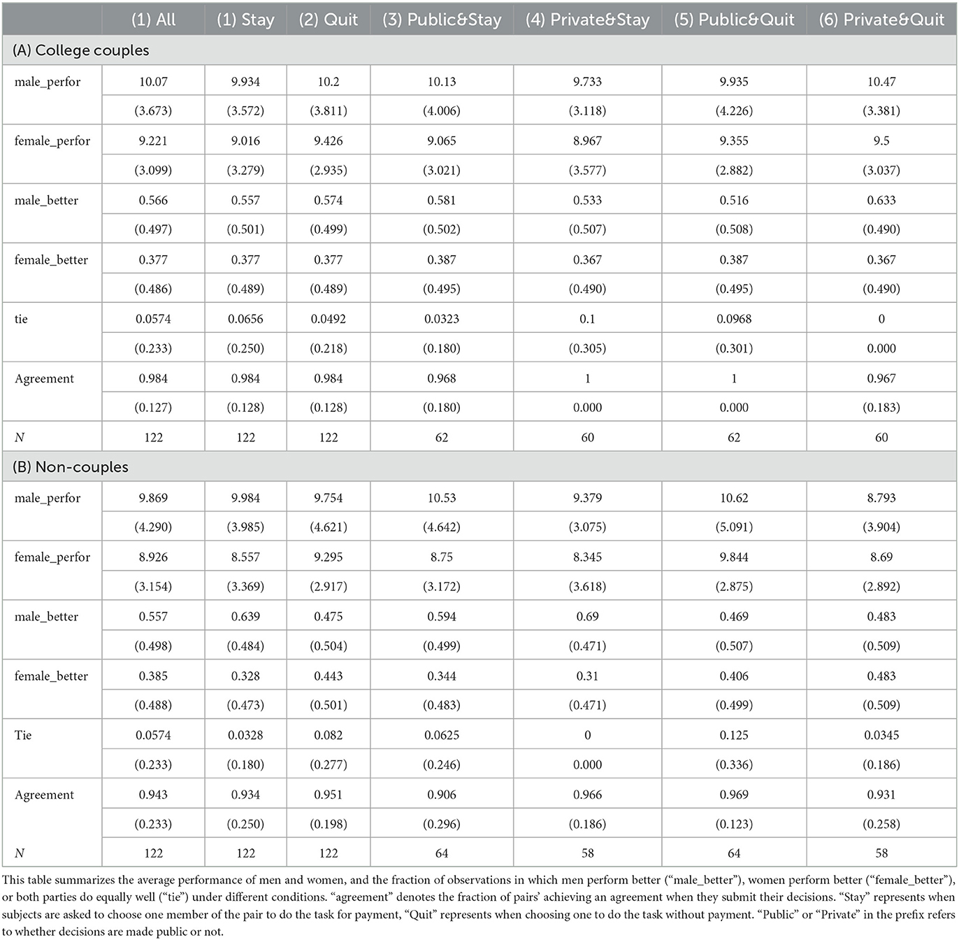
Table 2. Summary statistics.
Within the couple sample, the difference is not significant at the 5% significance level in the Stay framing (p = 0.1418 in a two-sided t-test) or under the Quit framing (p = 0.2134). In the non-couple control sample, males' average performance is significantly better than females' in the Stay framing (p = 0.0348), while the performance difference is not significant under Quit (p = 0.5131). None of the differences are significant under a Wilcoxon rank-sum test (p = 0.2069 for couples in Stay and p = 0.4404 in Quit, p = 0.0.0548 for the non-couple control sample in Stay and p = 0.6712 in Quit).
4.3. Choices in the task allocation
Figures 4, 5 depict individuals' choices in both samples and framing conditions. When they were asked to choose a person to continue the task for payment, as Figure 4 illustrates, around 65% of couples chose the man in the pair to continue the task for payment. When asked to choose a person to work without payment, the majority of couples (72%) agreed on the woman in the pair. Only 1% of the couples delegated the computer to make the choice.
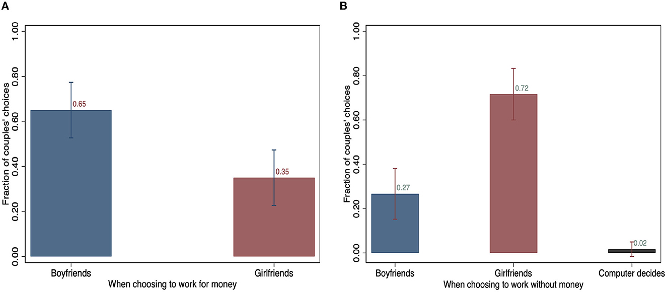
Figure 4. Couples' choices of whom to continue the task. (A) Continue the task for payment. (B) Continue the task without payment.
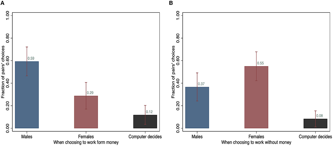
Figure 5. Non-couples' choices of whom to continue the task. (A) Continue the task for payment. (B) Continue the task without payment.
Among non-couples, about 58% chose the man to work for payment, and when choosing whom to work without payment, 55% selected the woman. Under both framings, a larger proportion of pairs in the non-couple sample delegated the computer to make the choice for them compared to the sample of couples.6 In Table 3, the variable “agreement” indicates the fraction of observations where both parties in the pair submit the same decision. On average, the agreement rate is high (over 93%) in both samples and under both framings. We fail to reject the hypothesis that the distribution of couples' and non-couple control sample's choices are the same under Kolmogorov -Smirnov tests (p = 0.346 for the Stay framing, and p = 0.529 for the Quit framing).
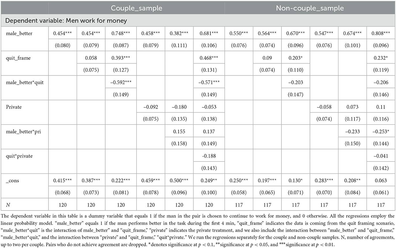
Table 3. Determinants of choices of who works for money, with better performance coded as a dummy variable.
4.4. Influences on the decision to stay on the job and to quit
In this subsection, we analyze the relationship between the relative performance of the pair and their choices. We first analyze the real-life couples. In the “Stay framing” scenario, men perform better than their partners in 57% of instances in the first round. Women perform better 37% of the time and the two parties perform equally in the remaining 6% of observations. In the “Quit framing” scenario, the pattern is similar. If couples are making decisions completely out of the efficiency concerns, that is, if they want to maximize their total material payoff, then we should find a similar distribution of couples' decisions. We cannot reject the null hypothesis that the proportion of couples that choose men to continue the task for payment is the same as the proportion of couples where men are better performers (p = 0.3497 under a Proportion test). However, the proportion of couples that choose women to continue the task without payment is significantly larger than the proportion of couples in which males are better performers (p = 0.0433 in the Proportion test). These findings imply that efficiency is not the only factor in couples' decisions, especially when they consider who to continue the task without payment, and that there is a bias in the direction of choosing the male partner.
Among our non-couple sample, in the “Stay framing” scenario, men are better performers in 63% of cases, women in 33% of instances and the two are tied in the remaining 4%. In the “Quit framing” scenario, the percentages are 47, 44, and 9% respectively. In the non-couple group, we fail to reject the null hypothesis that the proportion of pairs choosing males to continue the task for payment is the same as the proportion of pairs in which males perform better (p = 0.5654 in the Proportion test). Also, when asked to choose one person to continue the task without payment, we fail to reject the null hypothesis that the proportion of pairs choosing females to continue the task without payment is the same as the share of better performers who are female (p = 0.4614 in the Proportion test). This suggests that efficiency is the driving factor of choices in the non-couple, control, group.
Figures 6, 7 illustrate the individual-level relationship between relative performance in the pair and the pair's decision. Figure 6A, in each figure depicts couples' choices and Figure 6B represents non-couples'. For those pairs where the male is the better performer in the first 4 min, over 80% choose the male in the pair to earn the money for the group subsequently. Almost all couples (around 98%) select the man to continue the paid task if he performed better in the “Stay framing” scenario. In other words, when males perform better, only 2% of couples make the inefficient decision. When females earn more in the first round, around 24% of couples nevertheless choose the male to continue the work for payment. This indicates that when the female side has a larger relative earning potential, the pair is relatively more likely to make decisions that are not motivated by efficiency. For non-couples, the difference disappears as men are selected 88% of the time when they perform better, and women are chosen 90% of the time when they are the better performer.
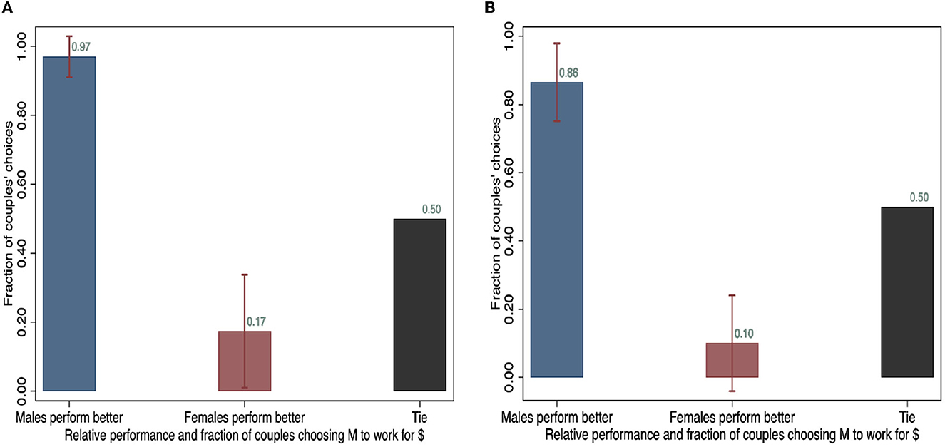
Figure 6. Relative performance and the share of pairs choosing men to work for money (“Stay framing” scenario). (A) Couples and (B) Non-couples.
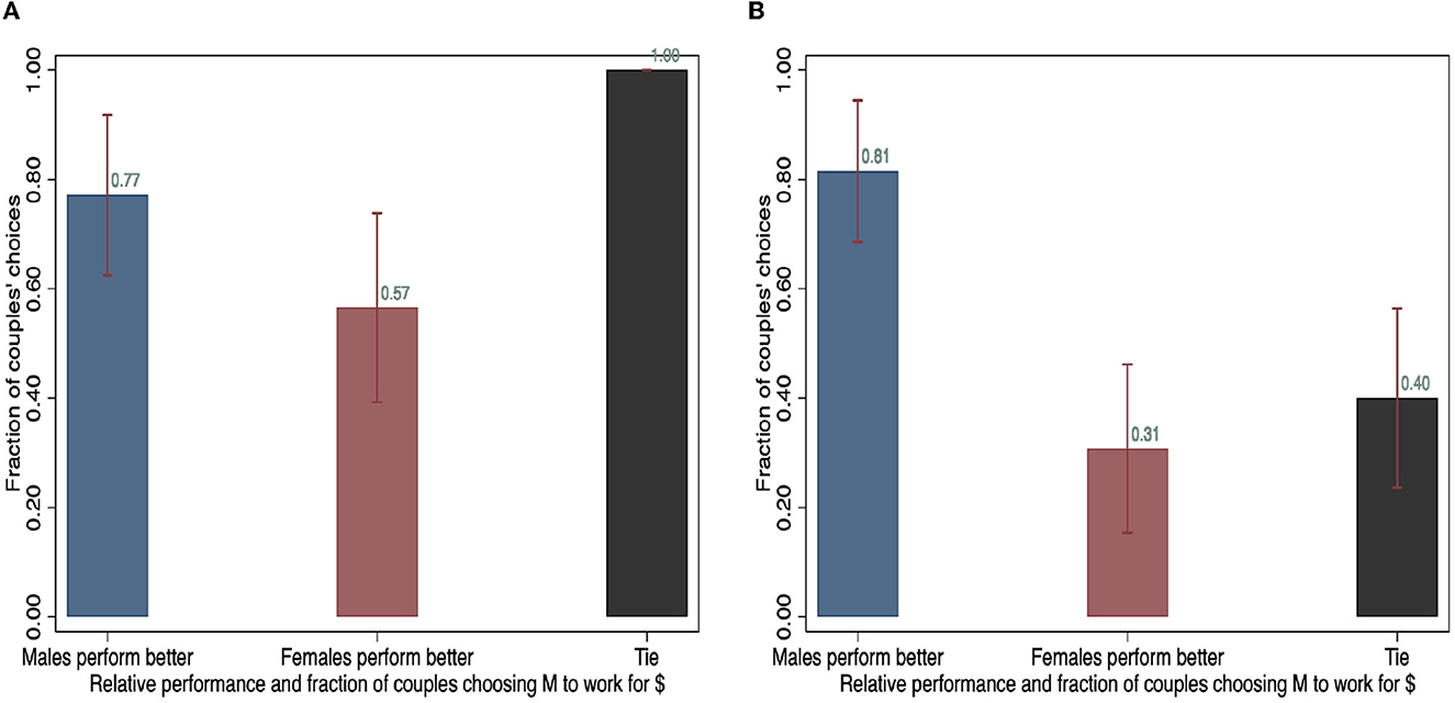
Figure 7. Relative performance and the share of pairs choosing women work for no money (“Quit framing” scenario). (A) Couples and (B) Non-couples.
In the “Quit framing” scenario, around 80% of couples choose the female to work without money when the male is better performers in the first round in both samples. This indicates that 20% of couples in which males are better performer make inefficient choices. However, over 50% of couples still choose females to continue the task without payment even if females perform relatively better in the first round. Thus, as in the “Stay framing,” when the female performs better, couples are much more likely to make inefficient choices. The number of pairs choosing females to quit even if they earn more decreases to 25% for non-couples, compared to the fraction of males who perform better (19%).
Tables 3, 4 report regression results that reveal the determinants of players' decisions. The unit of observation is the matched pair of players. Only pairs who came to an agreement are included in the estimation. The dependent variable equals 1 if the man continues to work for money and 0 if the woman does. The tables are the same with one exception. Table 3 includes a dummy variable, male_better that equals 1 if the man performed better than the woman before the decision was made, while Table 4 contains a variable perf_diff that equals the man's performance minus the woman's.
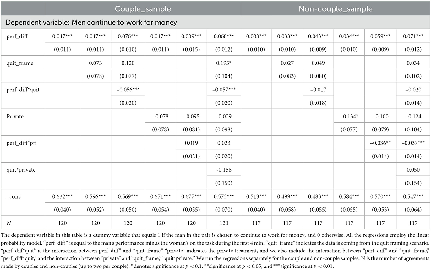
Table 4. Determinants of choices of who works for money, with relative performance as an independent variable.
The tables reveal consistent patterns. Both the male_better and the perf_diff variables are positive and significant under all specifications, indicating that efficiency is a strong consideration. An individual is more likely to be chosen to continue the better their performance compared to their partner, all else equal.
The positive and significant constant term reveals the extent of the bias toward men. In Table 3, in the left-most column in the first panel, the constant term is equal to 0.415 and significant. This means that in a couple, even when the woman is the better performer, the man still has a 41.5% chance of being chosen to work for money. When he is the better performer, he has a 86.9% chance (the sum of the coefficients on the constant term and male_better. In the control treatment, the first column of the right panel shows only a very small bias in that men are chosen 25% of the time when they are the worse performer and 80% of the time when they are better. In Table 4, the constant term reveals the likelihood that the man is chosen to continue to work for money when all other variables are 0. The first column of the table shows that for couples, the man is chosen 63.2% of the time when his performance is the same as his partners (when perf_diff = 0), but in only 51.3% of instances in the control group.
The quit_frame variable is significant as a main effect in some specifications, but not in others. Therefore, the evidence that framing affects the overall likelihood that the man remains in the labor force is in our view not compelling. The interaction terms male_better*quit and perf_diff*quit are consistently negative and significant, though modest in magnitude. These estimates suggest that performance is a somewhat less important a factor in the pair's decision under the Quit framing. Making decisions public also does not have a significant effect.
4.5. Relation between beliefs and decisions
In this subsection, we study the relationship between the gender norm an individual indicates to be present and their choices about who should continue to work. We find that couples with a male partner who believes in the social appropriateness of a man working for money and for a woman to work without money are more likely to choose the man to work for money. Non-couples are more likely to choose the man to work for money if both parties believe in the appropriateness of men earning money for a couple.
Table 5 reports regression estimates of the relationship. The pair is the unit of observation. The regressions employ the linear probability model. The variable “only_men_traditional” equals to 1 if the man in the pair holds the opinion that the norm is that men should be the main breadwinners and women should do unpaid work, as indicated in their responses on the questions asking about social appropriateness. “only_women_traditiona” and “both_gender_traditional” are dummy variables that equal 1 if only the woman holds, or both parties hold, this opinion respectively.
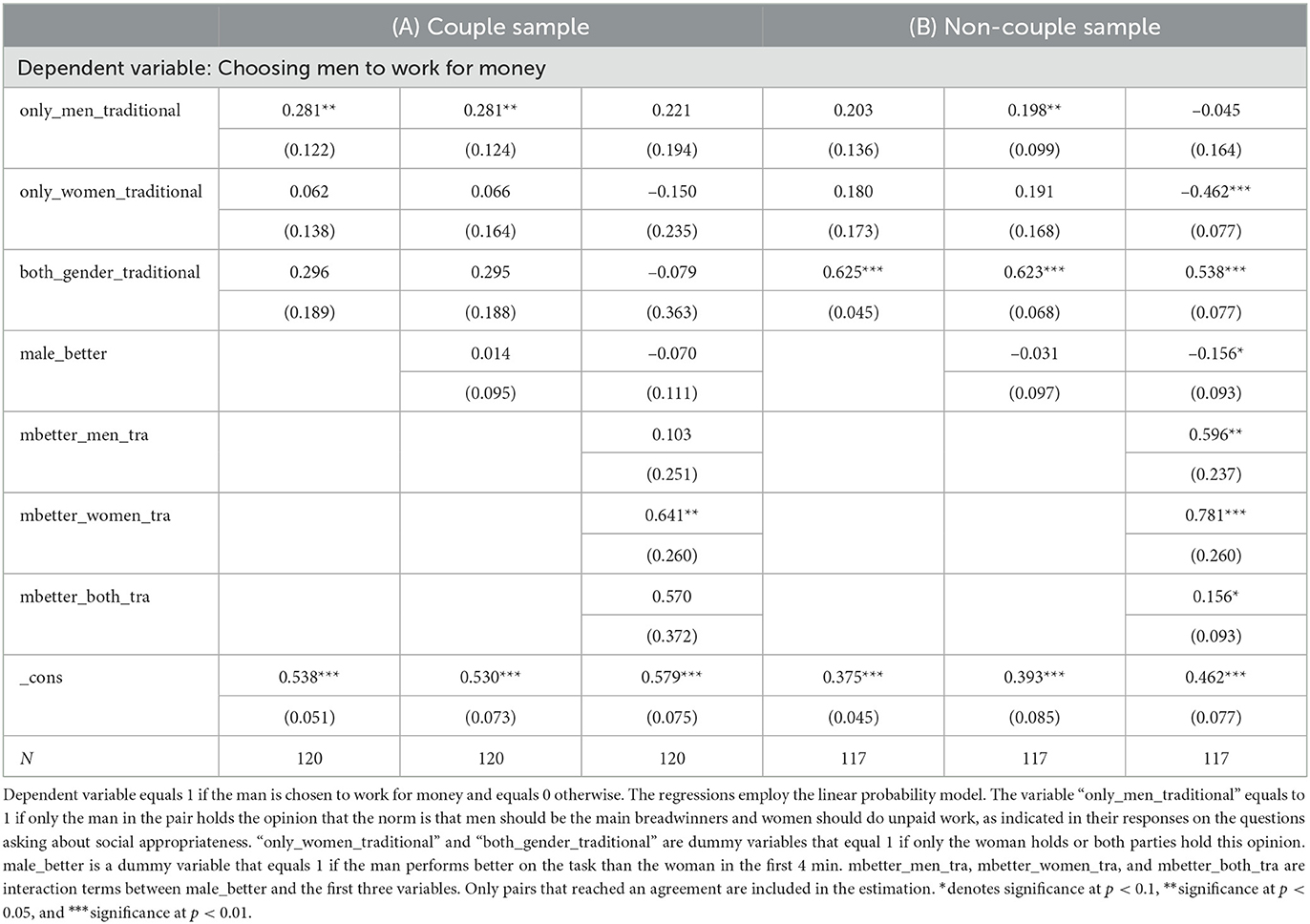
Table 5. Regression results on gender norm attitudes and choices.
The results reveal that for couples, pairs with a man who believes that men should continue to work and that women should quit are more likely to choose the male in the group to continue the task for money. This is apparent from the significance of the “only_men_traditional” variable in two of three specifications. For non-couples, the variable “both_gender_traditional” is significantly positive in all three specifications, indicating that in a non-couple, both parties have to be believe in the appropriateness of the traditional norm for it to be applied. The interaction term “mbetter_women_tra” is significant for both groups. This means that the more that the woman in the pair believes in the traditional norm, the more weight they put on relative performance in choosing who should work for money. For non-couples, we observe the same effect of the interaction between men's beliefs and relative performance.
5. Discussion
In our experiment, we found that in a large majority of instances, when the couple had to choose one individual to work for money and the other to work without monetary compensation, a significant majority chose the man to be the breadwinner. This is the case even though there is no gender difference in the average disutility of doing the task or in preference for being in the role of money-earner. This pattern is specific to couples, as our control treatment with non-couples showed this tendency much less strongly.
The likelihood of choosing the man in a couple as the wage-earner has a number of determinants. It is more likely when the man performs better in the task than the woman, indicating that efficiency is an important consideration. Nevertheless, there is a strong bias toward choosing the man to continue and the woman to quit the job, and when they have comparable ability, the man is selected in the majority of instances. Those couples where the man believes more strongly that a norm exists for men to continue to work are more likely to keep the man in paid work.
The patterns that we have observed fit into the previous literature and reinforce some earlier results. As emphasized by Goerges and Nosenzo (2020), we observe that norms affect labor market behavior. We also observe that outcomes are often inefficient, a theme of the survey of Munro (2018). We also observe, as do Görges (2015), Görges (2019), and Roncolato and Roomets (2020) that there is a bias toward choosing men to work at a paid activity and for women to work in an unpaid supporting role. In the Görges (2015) experiment, the experimenter imposes gains from specialization, and in that situation, couples generate greater efficiency than non-couples, overcoming the cost of the bias of choosing males to work for money too often. Here, in contrast, without such gains from specialization, the bias toward choosing men to work for money leads to inefficiency. Actual earnings of our couples are 12.1% and 12.4% lower under the Stay and Quit framing, respectively, then they would be if they had always chosen the better performer to continue the task.7 The earnings of non-couples are comparable, with efficiency losses of 17.2 and 18.8% in the Stay and Quit framings, respectively.
The results of our survey of a sample of the Chinese population and from Experiment 1 confirm that the norm is strong. The survey results are reported in Appendix D. The responses to the survey reveal that more that 23 times more men agree (either strongly or somewhat) than disagree with the statement “It's more appropriate for husbands to work outside the home to earn money and for wives to do the housework.” More than 3 times as many women agree than disagree with the statement as well. More 40 times as many men and 5 times as many women agree than disagree with the statement “Females are better than males at taking care of children.”
The data from the auxiliary Experiment 1 rule out two important explanations for the bias toward men continuing to work for money. There was no significant gender difference in the disutility of the task. This means that the fact that more men than women continued the task for money cannot be attributed to the fact that they disliked the task on average less than women. Such a difference would have provided a type of efficiency rationale for men to continue with the task for money and for women to opt out.
Another possible explanation for the selection of men to continue the task is the possibility that men prefer to have their own performance determine the outcome more strongly than women. However, the data from Experiment 1 refute this account. We measured individuals' willingness-to-pay to be the money-earner for the pair. There were no significant differences between women and men. This means that couples were not more likely to choose a man to earn money because men's preference for being in that role was stronger than women's. Rather, it does appear that the couple was adhering to a norm that men should be the money-earner for the couple.
Comparing the results of Experiment 1 in China and the US reveals only modest differences in attitudes in the two countries. Chinese respondents say that it is worse for an individual to work without payment, regardless of whether the individual is a woman or a man, than Americans do. Both groups have a strong tendency to believe that a man working for money is behaving more appropriately than a woman working for money. In both countries, the gender differences were smaller when girlfriends and boyfriends, rather than wives and husbands, were being considered. Chinese subjects have a greater tendency to be unwilling to pay any money to avoid the task, submitting more bids of 0 than American participants in Part B of Experiment 1.
6. Conclusion
The COVID-19 pandemic has highlighted a phenomenon that is troubling for gender equality. When a situation arises in which one member of a couple must exit the workforce, there is tendency for the woman in the couple to do so. Our experiment 1 reveals how strong the norm is that the man should remain the breadwinner in such a situation. Both in China and in the US, there is a strong belief among the student population that we studied, that this is the socially appropriate course of action. Our survey of a demographically representative sample of the Chinese population obtains a similar result.
The results from our main experiment reflect this norm. Among our real-life couples, the man in the couple was chosen to be the breadwinner in a majority of instances. This was true regardless of whether the decision was framed as quitting or as staying in a job, or whether it was publicly observable or not. Among non-couples, the tendency for a man to be the breadwinner is much less pronounced.
The results of this study starkly illustrate a difficult societal challenge. When one member of a couple must quit their job, there is a tendency for it to be the woman in the couple. Exiting the labor force, even temporarily, can often be very costly for career advancement and lower lifetime income considerably. The bias toward men continuing to work appears to be a strong societal norm, even among the relatively youthful and educated subjects of our study. Since norms are difficult to change, it will be a challenge to achieve gender equality in this area.
Data availability statement
The raw data supporting the conclusions of this article will be made available by the authors, without undue reservation.
Ethics statement
The studies involving human participants were reviewed and approved by University of Arizona Institutional Review Board. The patients/participants provided their written informed consent to participate in this study.
Author contributions
All authors listed have made a substantial, direct, and intellectual contribution to the work and approved it for publication.
Acknowledgments
The authors thank the laboratory at the China Center of Behavioral Economics and Finance (CCBEF) at the Southwestern University of Finance and Economics for permitting us to run sessions there. We are grateful to Lawrence Choo, Martin Dufwenberg, Erin Krupka, Senran Lin, Juan Pantano, Julian Romero, Evan J. Taylor, and Tiemen Wouterson, as well as seminar participants at CCBEF and the International Conference RExCon21 on Social Preferences and Social Norms for helpful comments.
Conflict of interest
The authors declare that the research was conducted in the absence of any commercial or financial relationships that could be construed as a potential conflict of interest.
Publisher's note
All claims expressed in this article are solely those of the authors and do not necessarily represent those of their affiliated organizations, or those of the publisher, the editors and the reviewers. Any product that may be evaluated in this article, or claim that may be made by its manufacturer, is not guaranteed or endorsed by the publisher.
Supplementary material
The Supplementary Material for this article can be found online at: https://www.frontiersin.org/articles/10.3389/frbhe.2023.1112934/full#supplementary-material
Footnotes
1. ^In our study, we restrict attention to heterosexual couples.
2. ^It has been proposed that the power of social norms comes from (1) the willingness of people within the population to punish (reward) others' deviation from (adherence to) the norms, as well as from (2) the experience of positive or negative emotions produced by one's own adherence or deviation from a social norm (Elster, 1989; López-Pérez, 2008).
3. ^We also conducted Experiment 1 in the US with American undergraduate students as participants. The results are reported in Appendix C. We also commissioned a survey of a demographically representative sample of Chinese citizens. These data are presented in Appendix D.
4. ^As in Krupka and Weber (2013), we explained to subjects that “socially appropriate” meant “consistent with moral or proper social behavior,” and “socially inappropriate” was “inconsistent with moral or proper social behavior”.
5. ^The framing sequence assignment was on the session level.
6. ^We reject the null hypothesis that choices are uniform across all options by performing a chi-squared test of frequency for couples (p = 0.000 for both framings), and for non-couples (p = 0.000 for both framings).
7. ^This calculation is made under the assumption that both individuals would continue to exhibit the same performance as in the first 4 min.
References
Abeler, J., Falk, A., Goette, L., Huffman, D. (2011). Reference points and effort provision. Am. Econ. Rev. 101, 470–492. doi: 10.1257/aer.101.2.470
Akerlof, G. A., Kranton, R. E. (2010). Identity Economics: How Our Identities Shape Our Work, Wages, and Well-Being. Princeton University Press, Princeton, NJ, United States.
Albanesi, S., Kim, J. (2021). Effects of the COVID-19 recession on the us labor market: occupation, family, and gender. J. Econ. Perspect. 35, 3–24. doi: 10.1257/jep.35.3.3
Becker, G. S. (1973). A theory of marriage: Part i. J. Polit. Econ. 81, 813–846. doi: 10.1086/260084
Bertrand, M., Kamenica, E., Pan, J. (2015). Gender identity and relative income within households. Q. J. Econ. 130, 571–614. doi: 10.1093/qje/qjv001
Cochard, F., Couprie, H., Hopfensitz, A. (2018). What if women earned more than their spouses? an experimental investigation of work-division in couples. Exp. Econ. 21, 50–71. doi: 10.1007/s10683-017-9524-5
Elster, J. (1989). Social norms and economic theory. J. Econ. Perspect. 3, 99–117. doi: 10.1257/jep.3.4.99
Fischbacher, U. (2007). z-tree: Zurich toolbox for ready-made economic experiments. Exp. Econ. 10, 171–178. doi: 10.1007/s10683-006-9159-4
Fortin, N. M. (2005). Gender role attitudes and the labour-market outcomes of women across OECD countries. Oxford Rev. Econ. Policy 21, 416–438. doi: 10.1093/oxrep/gri024
Fortin, N. M. (2015). Gender role attitudes and women's labor market participation: opting-out, aids, and the persistent appeal of housewifery. Ann. Econ. Stat. 117/118, 379–401. doi: 10.15609/annaeconstat2009.117-118.379
Goerges, L., Nosenzo, D. (2020). “Social norms and the labor market,” in Handbook of Labor, Human Resources and Population Economics, ed K. F. Zimmermann (London: Springer Nature publishers), 1–26.
Görges, L. (2015). The power of love: a subtle driving force for unegalitarian labor division? Rev. Econ. Househ 13, 163–192. doi: 10.1007/s11150-014-9273-6
Görges, L. (2019). Wage earners, homemakers &gender identity-using an artefactual field experiment to understand couples' labour division choices. Technical report, Working Paper.
Görges, L. (2021). Of housewives and feminists: Gender norms and intra-household division of labour. Labour. Econ. 72, 102044. doi: 10.1016/j.labeco.2021.102044
Hopfensitz, A., Munro, A. (2020). “Behavioral household economics,” in Handbook of Labor, Human Resources and Population Economics, ed K. F. Zimmermann (London: Springer Nature publishers) 1–21.
Krupka, E. L., Weber, R. A. (2013). Identifying social norms using coordination games: why does dictator game sharing vary? J. Eur. Econ. Assoc. 11, 495–524. doi: 10.1111/jeea.12006
Lezzi, E., Fleming, P., Zizzo, D. J. (2015). “Does it matter which effort task you use? A comparison of four effort tasks when agents compete for a prize,” in Working Paper series, University of East Anglia, Centre for Behavioural and Experimental Social Science (CBESS) 15–05. School of Economics, University of East Anglia, Norwich, United Kingdom.
López-Pérez, R. (2008). Aversion to norm-breaking: a model. Games Econ. Behav. 64, 237–267. doi: 10.1016/j.geb.2007.10.009
Mailath, G. J., Zemsky, P. (1991). Collusion in second price auctions with heterogeneous bidders. Games Econ. Behav. 3, 467–486. doi: 10.1016/0899-8256(91)90016-8
Munro, A. (2018). Intra-household experiments: a survey. J. Econ. Surv. 32, 134–175. doi: 10.1111/joes.12196
Noussair, C. N., Seres, G. (2020). The effect of collusion on efficiency in experimental auctions. Games Econ. Behav. 119, 267–287. doi: 10.1016/j.geb.2019.11.002
Roncolato, L., Roomets, A. (2020). Who will change the “baby?” examining the power of gender in an experimental setting. Rev. Econ. Househ. 18, 823–852. doi: 10.1007/s11150-020-09490-2
Keywords: gender identity, social norm, intra-household labor allocation, COVID-19 impact, experiment
Citation: He S and Noussair CN (2023) Social norms and couples' division of labor. Front. Behav. Econ. 2:1112934. doi: 10.3389/frbhe.2023.1112934
Received: 30 November 2022; Accepted: 02 February 2023;
Published: 22 February 2023.
Edited by:
Siri Isaksson, Norwegian School of Economics, NorwayReviewed by:
Rodolphe Dos Santos Ferreira, Université de Strasbourg, FranceAlexander Koch, Aarhus University, Denmark
Copyright © 2023 He and Noussair. This is an open-access article distributed under the terms of the Creative Commons Attribution License (CC BY). The use, distribution or reproduction in other forums is permitted, provided the original author(s) and the copyright owner(s) are credited and that the original publication in this journal is cited, in accordance with accepted academic practice. No use, distribution or reproduction is permitted which does not comply with these terms.
*Correspondence: Charles N. Noussair,  Y25vdXNzYWlyQGVtYWlsLmFyaXpvbmEuZWR1