Vague language and context dependence

In this paper, we broaden the existing notion of vagueness to account for linguistic ambiguity that results from context-dependent use of language. This broadened notion, termed literal vagueness, necessarily arises in optimal equilibria in many standard conversational situations. In controlled laboratory experiments, we find that, despite the strategic complexity in its usage, people can indeed use literally vague language to effectively transmit information. Based on the theory and the experimental evidence, we conclude that context dependence is an appealing explanation for why language is vague.

JEL classification numbers: C91, D03, D83.

1. Introduction

Language is vague, as this very sentence exemplifies (what does “vague” mean here, after all?), but we do not quite know why. On one hand, vagueness decreases accuracy and causes confusion; on the other hand, there seems to be no obvious benefit to vagueness that justifies its prevalence. Indeed, as Lipman (2009) forcefully argues, vagueness has no efficiency advantage in a game-theoretic model of communication if agents are rational. Thus, Lipman (2009) suggests, it seems that the presence of vagueness can be explained only if some of the agents are not entirely rational.

In this paper, we also attempt to explain vagueness. Rather than following the agenda of Lipman (2009), we instead maintain the rationality assumption but broaden the notion of vagueness. Language is defined as vague¹ if words are not divided by sharp boundaries—the set of objects described by a word may overlap with that described by another word. For instance, “red” and “orange” overlap in describing reddish-orange colors. We find this definition restrictive in that it rules out languages that would appear to people as vague. In particular, we observe that a word's operational meaning often depends on the context in which the word is used. Even if words are divided by sharp boundaries in every context, these boundaries may vary with the context and become fuzzy if the context is not clear to the listener, thereby creating a sense of vagueness, despite the fact that the language is technically not vague. In short, context-dependent use of words can cause a language to be perceived as vague. Based on this observation, we define a new notion, literal vagueness, which accommodates not only conventional vagueness but also context dependence.²

We show that literal vagueness can, and often does, have an efficiency advantage, in the sense that the optimal language in the standard model of information transmission is often literally vague. This is particularly the case when the information to be transmitted has some “unspeakable” aspects that are not explicitly describable by the available vocabulary. These aspects constitute the context. A literally vague language is more efficient because it is more capable of conveying information about the context than a literally precise language is.

Thus, a literally vague language is more efficient—but is this why everyday language is (literally) vague? We should note that a literally vague language might be difficult to use in reality because it requires complex strategic thinking. Our proposition, that the efficiency advantage of literal vagueness provides some explanation for why language is vague, would be greatly weakened if the strategic hurdle were so high that people could not effectively communicate with a literally vague language. With this concern in mind, we conducted a series of experiments to explore whether efficient literal vagueness would, as theory predicts, emerge in real conversations. We found that indeed it did.

In the experiments, we considered a conversational environment in which two speakers speak sequentially to a listener and the way that the later speaker uses his words may rely on what the earlier speaker said. In this simple environment in which the optimal language is literally vague, we observed that subjects indeed tended to communicate in such a way. By considering several variations of the environment with varying degrees of complexity in coordinating on the optimal language, we found that a literally vague langue was more likely to emerge when the net benefit from vagueness was larger and the environment was less complex.

In this paper, we suggest an explanation for why language is vague, and report evidence supporting the theory. However, we do not claim to have completely answered the question, and we are aware of the limits of the explanatory power of literal vagueness. On the theory side, we observe that language can be vague even when context dependence is not a concern, especially when full rationality is not guaranteed. On the experiment side, the observation that people can communicate with a literally vague language does not identify the efficiency advantage of literal vagueness as the explanation for the omnipresence of vague languages. Nevertheless, we believe that our exercise is a worthwhile step toward understanding vagueness.

In Section 2, we discuss the theoretical aspects of vagueness and literal vagueness. Section 3 describes the experimental design. In Section 4, we report the experimental findings. The related literature is discussed in Section 5. Section 6 concludes. In the Appendix, we include additional details on the experiments as well as some figures and tables.

2. Vagueness and literal vagueness

In this section, we first discuss the formal game-theoretic definition of vagueness. Then, we illustrate why this definition is restrictive and introduce a broader notion: literal vagueness. Finally, we show that the optimal language in many communication situations must be literally vague.

2.1. Vagueness

In the standard communication model, a speaker who is informed about the state of the world ω ∈ Ω wishes to transmit this information to an uninformed listener. The speaker transmits the information by sending the listener a message from a message set M. Given the message, the listener chooses an alternative from a set A. For simplicity, assume that Ω, A and M are finite. Conditional on state ω and the listener's choice a, both players receive the same payoff of u(ω, a).³

In this setting, the language is the speaker's message-sending strategy λ:Ω → Δ(M), where Δ(M) is the set of all lotteries over M. As the speaker observes that the state is ω, he uses the lottery λ(ω) to draw a message to send to the listener.

The game-theoretic notion of what it means for a language to be vague or precise is due to Lipman (2009): Language λ is vague if it is a non-degenerate mixed strategy, or if otherwise the language is precise. This definition captures the essence of vagueness vis-à-vis precision: If λ is a non-degenerate mixed strategy, then multiple messages may be used to describe the same state. Thus, the boundaries between messages are not always sharp. In contrast, if λ is a pure strategy, then no such overlapping exists and the boundaries between messages are sharp.

Given language λ, let π_λ(m) denote the set of states in which message m is sent with positive probability. It is clear that Π_λ: = {_{πλ(m)}m ∈ M} is a covering of Ω, and moreover, Π_λ is a partition of Ω if λ is precise. In our further analysis, this partition Π_λ will serve as a useful representation of a precise language λ.

The central thesis of Lipman (2009) is that vagueness has no efficiency advantage over precision because there is always a precise language among the optimal equilibrium languages in any communication setting.

2.2. Literal vagueness

The following example demonstrates that the definition of vagueness provided above does not capture a certain degree of vagueness in speech.

Example 1. In a conference, a presenter, Bob, asks an audience member, Alice, “How was my talk?” Alice's reply depends on 1) whether she likes Bob's research (L) or not (NL) and 2) whether she has time for further conversation (T) or is in a hurry to the next session (NT). If Alice does not have time, she says “It was interesting.” (l). If she has time, she says “It was interesting” if she likes the talk or “Here are a few things you could try” (nl) if she is less certain about Bob's research.

Is Alice's language vague? This example is formalized with the state set Ω = {L,NL} × {T, NT} and the message set M = {l, nl}. Alice's language is precise by definition because she uses the message nl with certainty in state (NL, T) and message l with certainty in other states. Her language nonetheless “sounds” vague: If she says “It was interesting,” either she may like Bob's research or she may not and is just in a hurry to end the conversation.

If Alice's language is precise, where does the sense of vagueness originate? Observe that the messages “It was interesting” and “Here are a few things you could try” literally concern Bob's research only and are irrelevant to Alice's hurriedness. Alice's language is precise with respect to the states, but is not precise with respect to how she likes Bob's research. The sense of vagueness comes from the language's failure to unambiguously describe the particular aspect of the state the messages are literally intended to describe.

Languages such as Alice's are deemed to be precise by the formal definition because in the standard model of conversation, Ω and M are abstract sets that lack structure and relation. Within the model, there is no linguistic convention, and hence, no exogenous literal interpretation exists apart from the speaker's idiosyncratic use of the messages. In other words, interpretation is purely endogenous. In contrast, a word in a natural language is literally intended to describe a particular aspect of the world, e.g., color or height. A sense of vagueness could occur if there is inconsistency between the literal interpretation and an individual's idiosyncratic language use, as is the case in Example 1.

This observation motivates us to modify the standard setting to incorporate an exogenous literal interpretation. Suppose the state set now has a two-dimensional product structure such that Ω = F × C. For any ω = (f,c) ∈ Ω, f is called the feature of the state and c the context. Messages in M literally describe features but not contexts. In Example 1, we have F = {L, NL}, C = {T, NT} and M = {l, nl} because the messages literally concern only Alice's attitude toward Bob's research.

A new notion of vagueness can thus be defined as follows. A language λ is said to be literally vague if it satisfies one of the following two conditions:

L1. λ is vague.

L2. There exist distinct f, f′ ∈ F and distinct c, c′ ∈ C such that λ(f, c) = λ(f′, c′) and λ(f, c) ≠ λ(f, c′).

Otherwise, we say λ is literally precise.⁴

According to L1, a vague language is literally vague. L2 is novel: It implies that boundaries between messages with respect to features vary with the context. To see this, suppose that λ is precise but satisfies L2. The same message m describes both states (f, c) and (f′, c′), while a different message m′ describes state (f, c′). Observe that m and m′ overlap in describing the feature f, although these two messages do not overlap in describing the states.

Returning to Example 1, Alice's language is literally vague because λ(L, T) = λ(NL, NT) = l yet λ(L, T) ≠ λ(L, NT) = nl. The boundary between messages l and nl is not sharp regarding Alice's attitude toward Bob's research, as when Alice has doubts (NL obtains), she sometimes uses nl vis-à-vis l to clearly express them but sometimes uses nl regardless of her attitude.

The following lemma presents a useful representation of a literally precise language using the partitional knowledge structure it induces for the listener.

Lemma 1. A precise language λ is literally precise if and only if every π ∈ Π_λ is the Cartesian product of a subset of F and a subset of C.

Proof. Take a precise language λ. The “if” direction is immediate. Suppose λ is literally precise. For any π ∈ Π_λ, let $\widehat{F}$ denote the projection of π to F and Ĉ the projection of π to C. Pick any $f\in \widehat{F}$ and c′ ∈ Ĉ. For any c ∈ C where (f, c) ∈ π and f′ ∈ F where (f′, c′) ∈ π, we have λ(f, c) = λ(f′, c′), which in turn implies λ(f, c′) = λ(f, c) because L2 is not satisfied. It follows that π is the product of its projections to F and C, proving the “only if” direction.□

This representation has a clear interpretation: In a literally precise language, the set of features described by a message remains the same regardless of the context.

2.3. Literal vagueness and context dependence

We see that literal vagueness prevails only if the set of features described by a message is context dependent. However, context dependence does not necessarily imply literal vagueness. For example, the same person may be referred to as Mark Twain or Samuel Langhorne Clemens depending on the context. This type of context dependence not necessarily cause literal vagueness, because distinct messages may simply convey variation in the context but not variation in the feature. In situations of context dependence that cause literal vagueness, the speaker chooses the same message to describe different sets of features depending on the context.

Context dependence and, hence, literal vagueness arise from the need to convey information not only about features but also about contexts when the available language is limited, in the sense that it literally describes features only.⁵ A natural question immediately follows: Why not use a richer language that also includes words that literally describe the context? Below, we provide a few reasons.

The first reason is that the environment of the conversation restricts the language to only describe features, particularly if the sender responds to a question framed in a certain way. Example 1 illustrates this case: Alice responds to Bob's question about his research and, therefore, appropriately uses messages that literally concern only this aspect.⁶

Second, in certain situations, a richer language does not exist. For example, the common language shared by people from different linguistic backgrounds is limited. People with different native tongues can use a facial expression in person or emojis ☺ / emoticons :-) on the internet as a common language to describe an emotion, but this common language lacks terms that describe any other aspect of the world.

The third reason is that the context is sometimes meta-conversational,⁷ i.e., it includes information about the environmental parameters of the conversation itself. This information is usually not explicitly discussed in a conversation. Here, we give two elaborating examples.

Example 2. Alice wishes to describe to her tailor, Bob, the color she has in mind for her next dress. Alice may have a small vocabulary for colors that has only coarse terms such as “red” or “blue,” or she may have an extensive vocabulary that includes words to denote subtle colors such as “burgundy” and “turquoise.” Alice's vocabulary is unknown to Bob.

If Alice's vocabulary is rich, she uses “burgundy” for burgundy-red and “red” for red-red; if her vocabulary is poor, she uses “red” for both burgundy-red and red-red.

In this example, the subject matter of the conversation is color (the feature) and the environmental parameter of the conversation is Alice's vocabulary (the context). Because they are color terms, the messages are literally intended to describe the color, not Alice's vocabulary. It is easy to verify that Alice's language is literally vague.

This example is based on the model studied in Blume and Board (2013). In their model, the available messages may vary depending on the speaker's language competence. Obviously, the essence of their model can be embedded into ours by interpreting language competence as the context, and it follows that their notion of “indeterminacy of indicative meaning” translates into literal vagueness.

Example 3. Alice wishes to describe Charlie's height to Bob so that Bob can recognize Charlie at the airport and pick him up. Moreover,

• Alice knows whether Charlie is an NBA player.

• Bob may or may not know whether Charlie is an NBA player.

• Alice may or may not know whether Bob knows whether Charlie is an NBA player.

Alice describes whether Charlie is “tall” or “short.” If she believes Bob knows that Charlie is an NBA player, then she says Charlie is “tall” only if his height is above 6 foot 10, whereas if she believes Bob does not know that Charlie is an NBA player, then she says Charlie is “tall” only if his height is above 6 foot 2.

In this example, “tall” and “short” are messages that literally concern Charlie's height (feature), where Alice's belief about whether Bob knows that Charlie is an NBA player is the environmental parameter of the conversation and, hence, the context. Clearly, Alice's language is literally vague.

A more formal model for the example is as follows: The listener's knowledge about the payoff-relevant state set is not common knowledge. In particular, before the conversation, the listener may receive with some probability an informative private signal that narrows down the possible set of payoff-relevant states. Moreover, the speaker may also receive a private (possibly noisy) signal that tells him whether the listener has been given that informative signal. It is straightforward to construct a typical decision problem under which, in the optimal equilibrium, the meaning of a message from the speaker depends on the signal that he receives. If we do not incorporate the speaker's signal as part of the state, then the optimal language is vague. However, in the enriched model in which the speaker's signal is considered the context and the payoff-relevant state is considered the feature, the optimal language is not vague but is literally vague.

Example 3 and the general model described in the previous paragraph resemble the model studied by Lambie-Hanson and Parameswaran (2015) in which the speaker and the listener receive correlated signals about the listener's ability to interpret messages.

Finally, we show an example demonstrating that context may arise endogenously in a sequential communication procedure that resembles information cascade. When multiple speakers speak sequentially, the way later speakers talk may rely on what earlier speakers have said. Earlier messages become the context on which later messages depend—the context of the bilateral conversation between a later speaker and the listener is then endogenously generated in the larger-scale multilateral conversation.

Example 4. Alice and Bob interview a job candidate. Alice observes the candidate's ability, which is evaluated by a number A. Bob observes the candidate's personality, which is evaluated by a number B. The best decision is to hire the candidate if and only if A + B ≥ 100.

Alice and Bob sequentially report (with Alice speaking first) their observations to the committee chair, Charlie, who is to make the hiring decision. They report whether their respective observation is “high” or “low.”

Suppose A and B are uniformly and independently distributed on [0, 100]. The best strategy is the following: Alice reports “A is high” if A ≥ 50 and “A is low” otherwise. If Alice reports “A is high,” then Bob reports “B is high” if B ≥ 25 and “B is low” otherwise; if Alice reports “A is low,” then Bob reports “B is high” if B ≥ 75 and “B is low” otherwise. Charlie hires the candidate if and only if Bob reports “B is high.”

It is important to discuss in greater detail how Example 4 fits the simple baseline model we introduced at the beginning of the section because this game will be used as the benchmark model for our experiments that appear later. There are two types of equilibria in this game. In the first type of equilibria, Alice babbles, i.e., Alice's reports do not contain any useful information about the candidate's ability, the case in which context is not properly defined. In the second type of equilibria, however, Alice's reports are informative and thus provide the context in which Bob's report is to be correctly interpreted. Conditional on Alice's report being informative, the later-stage extensive subgame that starts with Bob's decision node can be formalized with the state set Ω = F × C and the message set M = {“B is high”, “B is low”}, where C = {“A is high”, “A is low”} and F = [0, 100].

2.4. The efficiency advantage of literal vagueness

We show that literally vague language may have an efficiency advantage over literally precise language. Therefore, the main result of Lipman (2009) is reverted as we broaden the notion of vagueness.

Proposition 1. Suppose |F| ≥ 2, |C| ≥ 2, |A| ≥ 2 and min{|F||C| − 1, |A|} ≥ |M| ≥ 2. There exists a payoff function u: Ω × A → ℝ under which the language in any optimal perfect Bayesian equilibrium must be literally vague.

Proof. Pick any payoff function u such that

U1. Every state has a unique optimal action.

U2. The set T_u: = {a ∈ A:ais the optimal action in some state ω ∈ Ω} has |M| elements.

U3. There is some a ∈ T_u such that the set $\widehat{\text{Ω}}(a):=\left\{\omega \in \text{Ω}:a\mathit{\text{ is the optimal action in }}\omega \right\}$ is not the Cartesian product of a subset of F and a subset of C.

U1 and U2 imply that states can be partitioned into |M| subsets such that states in the same subset share the same unique optimal action and states in different subsets differ in the optimal action. U3 implies that not every subset in this partition is the Cartesian product of a subset of F and a subset of C.

By U1 and U2, any optimal language is a bijection from $\left\{\widehat{\text{Ω}}(a):a\in T_u\right\}$ to |M|. Thus, ${\Pi }_{\lambda }=\left\{\widehat{\text{Ω}}(a):a\in T_u\right\}$. U3 and Lemma 1 thus imply that none of the optimal languages is literally precise.□

Remark 1. The conditions |F| ≥ 2, |C| ≥ 2 and |A| ≥ 2 reflect that the state set and the decision problem are not trivial. |M|≥2 reflects that communication is not trivial. |F||C| − 1 ≥ |M| implies that the perfect description of every state is impossible, that is, no one-to-one relation between states and messages exists. It is noteworthy that the whole issue of vagueness would be less of a concern if messages were not limited because the perfect description is best whenever feasible.

Remark 2. |A| ≥ |M| is not a necessary condition. The assumption is made to simplify the proof.

Remark 3. Note that Proposition 1 is robust to the players' prior beliefs because ex post optimality is achieved in any optimal equilibrium under the payoff function we construct. It follows that a potential ex ante conflict of interest due to heterogeneous priors becomes irrelevant concerning the optimal equilibria because they are the most preferred strategy profiles by both players regardless of priors. If we restrict the priors, for example, by assuming common prior, then the set of payoff functions under which Proposition 1 holds could significantly expand. Therefore, for literal vagueness to be optimal, conditions U1-U3 are sufficient but not necessary.

Remark 4. How common are payoff functions that satisfy the construction in the proof of Proposition 1? To get a sense of this answer, suppose |A| = |M| = 2. It is clear that a payoff function almost surely satisfies U1. Each payoff function u satisfying U1 induces a strict preference $\left\{{\succ }_u^{\omega }\right\}$ such that $a{\succ }_u^{\omega }{a}^{\prime }$ if and only if u(ω, a) > u(ω, a′) for any a, a′ ∈ A. There are a total of 2^|F||C| preference profiles inducible by a payoff function satisfying U1. Among these preference profiles, 2^|F||C|−2 imply U2. Further, among these, 2^|F|+2^|C|−4 violate U3. Therefore, the fraction of preferences satisfying U2 and U3 among those satisfying U1 ⁸ is

$\begin{array}{l}\frac{2^{|F||C|}-2^{\left|F\right|}-2^{\left|C\right|}+2}{2^{|F||C|}}.\hfill \end{array}$

This bound approaches 1 as |F| and |C| grow. Thus, for an environment with a large state space, it is very likely that the optimal language is literally vague.

Remark 5. Note that Examples 2 and 3 do not immediately fit in the standard model, because in the standard model, unlike in Example 2, the message set does not vary with the context, and unlike in Example 3, the listener does not receive a signal. Therefore, Proposition 1 does not immediately apply to these examples. It is nonetheless not difficult to tailor the model to these examples. In particular, Blume and Board (2013) present results in spirit similar to Proposition 1 for Example 2.

3. Experimental implementation

We have seen that literally vague languages can be more efficient than literally precise languages in transmitting information. However, using a literally vague language may be challenging in reality—it requires the speaker to adopt a more complicated strategy and the listener to expect that correctly. If the strategic hurdle is so high as to overshadow the efficiency advantage, then literal vagueness loses its appeal and is less likely to be a sensible explanation for the prevalence of vague languages. Hence, we want to investigate whether people can effectively use literally vague languages to communicate in reality. We design our experiments with this question in mind. Of course, a positive finding alone does not sufficiently prove that the prevalence of linguistic vagueness is founded on the efficiency advantage of literal vagueness in our sense, yet it is a worthwhile first step.

3.1. Experimental games

We use the situation described in Example 4 to examine whether, and if so, how, people use literally vague language in conversation. This example has a number of important and attractive features that make it particularly suitable for our purpose. First, as we show below, the optimal language, which is literally vague, has a moderate degree of efficiency advantage, which renders literal vagueness potentially useful but not entirely crucial for communication. Second, the situation is simple and straightforward, and thus, in principle, it should shorten the learning period and make the experimental results more similar to the eventual stable language, or in terms of Lewis (1969), the “convention.” Third, the situation covers the most general environment in which the context, that is, the message from Alice, is endogenously generated. Fourth, and most important, this game has different types of equilibria, one in which context is properly defined and another in which context does not emerge endogenously. So, the emergence of a context-dependent, literally vague language is not a necessary condition for an equilibrium. However, it is necessary that individuals in this communication environment use a literally vague language in the optimal equilibrium of the game.

3.1.1. The benchmark game

There are three players: two senders, Alice and Bob, and one receiver, Charlie. Alice privately observes a number A and Bob a number B. A and B are independently and uniformly drawn from [0, 100]. Alice sends a message to Bob, where the message is either “A is Low” or “A is High.” Alice's message is unobservable to Charlie. Then, Bob sends a message to Charlie, where the message is either “B is Low” or “B is High.” Charlie receives Bob's message (but not Alice's message) and chooses an action: UP or DOWN. Players' preferences are perfectly aligned. If A+B ≥ 100 and UP is chosen, or if A + B ≤ 100 and DOWN is chosen, then all receive a payoff of 1. Otherwise, all receive a payoff of 0.

Equilibria of the game can be classified into three categories:⁹

1. Bob babbling: Bob uses a strategy such that Charlie's posterior about A+B remains the same as the prior upon seeing any message chosen by Bob with positive probability. Whether Alice babbles or not does not bear on the outcome. No information is transmitted, and Charlie is indifferent between the two actions regardless of the message he receives. Accordingly, the success rate, which is the probability that Charlie chooses the optimal action, is 50%.

2. Alice babbling: Bob sends message “B is High” if B > 50 or “B is Low” if B < 50.¹⁰ Charlie chooses UP seeing “B is High” and DOWN otherwise. Only Bob's information is transmitted. Accordingly, the success rate is 75%.

3. No babbling: Alice sends “A is High” if A > 50 and “A is Low” if A < 50.

• If Alice's message is “A is High,” then Bob sends “B is High” if B > 25 and “B is Low” if B < 25.

• If Alice's message is “A is Low,” then Bob sends “B is High” if B > 75 and “B is Low” if B < 75.

Charlie chooses UP seeing “B is High” and DOWN otherwise. Accordingly, the success rate is 87.5%.

Clearly, any equilibrium in which no one babbles is optimal. Because the messages available to Bob explicitly refer to the value of B alone, Bob's language in any optimal equilibrium is clearly literally vague because the set of values of B that a particular message—say, “B is high”—describes depends on Alice's message, which serves as the context.

To best test whether the players indeed effectively use the optimal literally vague language, we consider the counterfactual in which they do not, which can be formally modeled as Bob being constrained to use the same messaging strategy regardless of Alice's message. In this case, the best Bob can do is to always use the cutoff of 50, and the corresponding success rate is 75%. To examine the results and test whether the counterfactual holds, we pay particular attention to how Bob's use of language depends on Alice's message.

In addition, for a literally vague language to be effectively used, the listener should also be aware of the underlying context dependence and correctly consider it when making decisions. However, Charlie's strategy in the counterfactual would be the same as that in an optimal equilibrium so that considering only the benchmark will not allow us to identify whether the listener fully understands the optimal, context-dependent language or not. Thus, we need further variations for sharper identification.

Variation 1 (Charlie hears Alice).

Consider a variation of the benchmark: The only difference is that Alice's messages are now also observable to Charlie. The equilibria in which no one babbles remain the same as in the benchmark. It is particularly notable that Charlie's strategy does not depend on Alice's message even though it is observable.

In this variation, if Charlie believes that Bob uses his language in the optimal, literally vague way, the former's choice should not depend on Alice's message because the information contained in Alice's message is fully incorporated into Bob's message through context dependence. Thus, we can tease out whether Charlie correctly interprets Bob's message according to the optimal language by checking whether Charlie's choice depends on Alice's message.

Variation 2 (Charlie chooses from three actions).

In this variation, Charlie has three actions to choose from: UP, MIDDLE and DOWN. UP is optimal if A+B ≥ 120, MIDDLE if 80 ≤ A+B ≤ 120, and DOWN if A+B ≤ 80. If the optimal action is chosen, the players all receive a payoff of 1 and 0 otherwise.

In equilibria in which no one babbles, Alice sends “A is High” if A > 50 and “A is Low” if A < 50.

• If Alice's message is “A is High,” then Bob sends “B is High” if B > 25 and “B is Low” if B < 25.

• If Alice's message is “A is Low,” then Bob sends “B is High” if B > 75 and “B is Low” if B < 75.

Charlie chooses UP seeing “B is High” and DOWN otherwise. Accordingly, the success rate is 63.5%. It should be noted that MIDDLE is never chosen in this equilibrium.

The purpose of introducing the third action is to make the conversational environment more complex, particularly for Bob and Charlie. The benchmark and Variation 1 are relatively simple environments in which it is not supremely difficult to “compute” the optimal cutoffs.¹¹ However, when people talk in real life, they do not typically derive the optimal language consciously. Thus, we aim to determine whether people can still arrive at the optimal, literally vague language and use it to effectively communicate when it is more difficult to explicitly derive the optimal language or whether they instead revert to context-independent language, which is simpler for the speaker to use and for the listener to understand. Thus, it is crucial to examine whether or not Bob's message is context dependent in this variation and whether Charlie best responds or not.

Variation 3 (Charlie chooses from three actions and hears Alice).

This variation differs from Variation 2 in that Alice's message is now observable to Charlie. In an optimal equilibrium, Alice sends “A is High” if A > 50 and “A is Low” if A < 50. Bob's strategy does not differ from that in Variation 2 qualitatively but has different optimal cutoffs.

• If Alice's message is “A is High,” then Bob sends “B is High” if B > 45 and “B is Low” if B < 45.

• If Alice's message is “A is Low,” then Bob sends “B is High” if B > 55 and “B is Low” if B < 55.

Charlie chooses UP seeing (“A is High,” “B is High”), DOWN seeing (“A is Low,” “B is Low”), and MIDDLE otherwise. The success rate is 78.5%. It should be noted that MIDDLE is chosen in this equilibrium when the messages from Alice and Bob disagree.

This variation serves two purposes. First, it allows us to study how the quantitative change in the optimal cutoff values affects language use. The optimal cutoff values that are substantially closer to one another generates a very minimal benefit of context dependence relative to the context-independent counterfactual. Second, this variation enables us to understand how individuals' choice of context-dependent languages is guided by the salience of incentives, given that the success rate from the context-independent counterfactual is 78%.

Variation 4 (Bob's Messages are Imperative).

Consider a variation of the Benchmark in which we replace Bob's messages “B is High” and “B is Low” by “Take UP” and “Take DOWN”. Clearly, this change eradicates any possibility of literal vagueness because Bob's messages, now imperative, have unambiguous literal interpretations with respect to the decision problem at hand. Apart from the difference in the literal interpretation of messages, the variation is the same as the benchmark. Hence, the variation serves as a useful control version of the benchmark. In particular, it allows us to test whether literal vagueness may intimidate players from using the optimal language.

In the experiments, we create not only an “imperative messages” version of the benchmark but also one of variation 2.

3.2. Experimental design and hypotheses

The benchmark game and its variants introduced in the previous section constitute our experimental treatments. Our experiment features a (2 × 2) + (2 × 1) treatment design (Table 1). The first treatment variable concerns the number of actions available to the receiver (Charlie), and the second treatment variable concerns whether or not Alice's messages are observed by Charlie. The third treatment variable concerns whether Bob's messages are framed to be indicative or imperative.¹² We consider the treatments with imperative messages as a robustness check and therefore omit the corresponding treatments in which Alice's messages are observed by Charlie.

TABLE 1

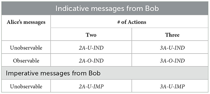
Table 1. Experimental treatments.

Note that we design our experiments to obtain empirical evidence on the efficiency foundation of literal vagueness. Hence, all our (null) hypotheses in this section are stated based on the assumption that the optimal equilibrium will be achieved in the laboratory. We pay attention to several properties of the optimal equilibrium (e.g., whether the observability of Alice's message to Charlie affects the success rate) and comparative statistics that result from the optimal equilibrium. Those properties do not necessarily hold in some other, Pareto-suboptimal equilibria.

Our first experimental hypothesis concerns the overall outcome of the communication games represented by the success rate. Let S(T) denote the average success rate of Treatment T. There are two qualitative characteristics predicted by the optimal equilibrium with context-dependent, literally vague language. First, the observability of Alice's message to Charlie does not affect the success rate in the treatments with two actions, while the same observability increases the success rate in the treatments with three actions. Second, the imperativeness of Bob's messages does not affect the success rate. Thus, we have the following hypothesis.

Hypothesis 1 (Success Rate).

1. Observability of Alice's message to Charlie does not affect the success rate in the treatments with two actions, i.e., S(2A-O-IND) = S(2A-U-IND).

2. Observability increases the success rate in the treatments with three actions, i.e., S(3A-O-IND) > S(3A-U-IND).

3. The imperativeness of Bob's messages does not affect the success rate, i.e., S(2A-U-IND) = S(2A-U-IMP) and S(3A-U-IND) = S(3A-U-IMP).

Our second hypothesis considers the counterfactual in which Bob is constrained to be context independent and thus always uses the cutoff of 50.¹³ In the counterfactual scenario, the success rates are 75% in Treatments 2A-O-IND, 2A-U-IND, and 2A-U-IMP, 78% in Treatment 3A-O-IND, and 55% in Treatments 3A-U-IND and 3A-U-IMP. If the players effectively use the optimal, literally vague language, the success rates should be significantly above the levels predicted by the counterfactual. Thus, we have the following hypothesis.

Hypothesis 2 (Counterfactual Comparison). The observed success rate in each treatment is significantly higher than the success rate calculated based on the counterfactual in which Bob is constrained to be context independent. More precisely,

1. S(2A-O-IND), S(2A-U-IND), S(2A-U-IMP) > 75%

2. S(3A-O-IND) > 78%

3. S(3A-U-IND), S(3A-U-IMP) > 55%

Note that the success rate predicted by the optimal, literally vague language in Treatment 3A-O-IND is 78.5%, which is not substantially different from the 78% predicted by the counterfactual. The net benefit of the context-dependent language measured with respect to the success rates is only 0.5% (= 78.5–78%) in Treatment 3A-O-IND. The net benefit of context dependence becomes substantially larger in other treatments as it is 12.5% (= 87.5–75%) in Treatments 2A-O-IND, 2A-U-IND, and 2A-U-IMP, and 6.5% (= 63.5–55%) in Treatments 3A-U-IND and 3A-U-IMP.

Our third hypothesis concerns Alice's message choices. For all treatments, the optimal equilibrium play predicts that Alice employs the simple cutoff strategy in which she sends “A is High” if A>50 and “A is Low” if A < 50. Let P_Alice(m|A) denote the proportion of Alice's message m given the realized number A. Then P_Alice(“A is Low”|A) = 1 for any A < 50 and P_Alice(“A is High”|A) = 1 for any A > 50.

Hypothesis 3 (Alice's Messages). Alice's message choices observed in all treatments are the same. Moreover, Alice employs the simple cutoff strategy in which she sends “A is High” if A > 50 and “A is Low” if A < 50.

Our next hypothesis concerns Bob's message choices. The optimal equilibrium play predicts that Bob's message choices depend on the context, i.e., which message he received from Alice. To state our hypothesis clearly, let $P_{Bob}^{m^{\prime }}(m|B)$ denote the proportion of Bob's message m given the realized number B and Alice's message m′ ∈ {“A is High, ” “A is Low”}. Define

$CD(B)=P_{Bob}^L(\overline{m}|B)-P_{Bob}^H(\overline{m}|B)$

where $\overline{m}$ is “B is Low” for the treatments with indicative messages and “Take DOWN” for the treatments with imperative messages. CD(B) measures the degree of context dependence of Bob's message choices given the realized number B. Bob's optimal, context-dependent strategy implies that there is a range of number B under which Bob's message choices differ depending on Alice's messages, i.e., CD(B) = 1. Such intervals are [45, 55] for Treatment 3A-O-IND and [25, 75] for all other treatments. It is worth noting that CD(B) = 0 for any B ∈ [0, 100] if Bob uses a context-independent strategy. Thus, we have the following hypothesis:

Hypothesis 4 (Bob's Messages). Bob's messages are context dependent in a way that is predicted by the optimal equilibrium of each game. More precisely,

1. For each treatment T, there exists an interval [X^T, Y^T] with X^T > 0 and Y^T < 100 such that CD(B) > 0 for any B ∈ [X^T, Y^T] and CD(B) = 0 otherwise.

2. The length of the interval [X^T, Y^T] is significantly smaller in Treatment 3A-O-IND than in any other treatment.

Our last hypothesis concerns whether the listener, Charlie, can correctly interpret the messages. In particular, Charlie's strategy in the optimal equilibrium does not depend on whether or not Alice's messages are observable to Charlie in the treatments with two actions. In the games with three actions, however, the observability of Alice's message to Charlie matters. Precisely, the optimal equilibrium predicts that MIDDLE should not be taken by Charlie in Treatments 3A-U-IND and 3A-U-IMP, whereas MIDDLE is taken in Treatment 3A-O-IND when the messages from Alice and Bob do not coincide. Thus, we have the following hypothesis.

Hypothesis 5 (Charlie's Action Choices). In the treatments with two actions, Charlie's action choices do not depend on whether Alice's messages are observable. In the treatments with three actions, MIDDLE is taken only in Treatment 3A-O-IND when the messages from Alice and Bob do not coincide.

3.3. Procedures

Our experiment was conducted in English using z-Tree (Fischbacher, 2007) at the Hong Kong University of Science and Technology. A total of 138 subjects who had no prior experience with our experiment were recruited from the undergraduate population of the university. Upon arrival at the laboratory, subjects were instructed to sit at separate computer terminals. Each received a copy of the experimental instructions. To ensure that the information contained in the instructions was induced as public knowledge, the instructions were read aloud, aided by slide illustrations and a comprehension quiz.

We conducted a session for each treatment. In all sessions, subjects participated in 21 rounds of play under one treatment condition. Each session had 21 or 24 participants and thus involved 7 or 8 fixed matching groups of three subjects: a Member A (Alice), a Member B (Bob), and a Member C (Charlie). Thus, we used the fixed-matching protocol and between-subjects design. As we regard each group in each session as an independent observation, we have seven to eight observations for each of these treatments, which provide us with sufficient power for non-parametric tests. At the beginning of a session, one-third of the subjects were randomly labeled as Member A, another third labeled as Member B and the remaining third labeled as Member C. The role designation remained fixed throughout the session.

We illustrate the instructions for Treatment 2A-U-IND. The full instructions can be found in Appendix A. For each group, the computer selected two integer numbers A and B between 0 and 100 (uniformly) randomly and independently. Subjects were presented with a two-dimensional coordinate system (with A in the horizontal coordinate and B in the vertical coordinate) as in Figures 5A, B in Appendix A. The selected number A was revealed only to Member A, and the selected number B was revealed only to Member B. Member A sent one of two messages—“A is Low” or “A is High”—to Member B but not to Member C. After observing both the selected number B and the message from Member A, Member B sent one of two messages—“B is Low” or “B is High”—to Member C, who then took one of two actions: UP or DOWN. The ideal actions for all three players were UP when A + B > 100 and DOWN when A + B < 100.¹⁴ Every member in a group received 50 ECU if the ideal action was taken and 0 ECU otherwise.

For Rounds 1-20, we used the standard choice method so that each participant first encountered a possible contingency and specified a choice for the given contingency. For example, Member A decided what message to send after seeing the randomly selected number A. Member B decided what message to send after observing the randomly selected number B and the message from Member A. Similarly, Member C decided what action to take after receiving the message from Member B. For Round 21, however, we used the strategy method and elicited players' beliefs by providing a small amount of compensation (in the range between 2 ECU and 8 ECU) for each correct guess.¹⁵ For more details, see the selected sample scripts for the strategy method and the belief elicitation provided in Appendix B.

We randomly selected two rounds of the 21 total rounds for each subject's payment. The sum of the payoffs a subject earned in the two selected rounds was converted into Hong Kong dollars at a fixed and known exchange rate of HK$1 per 1 ECU. In addition to these earnings, subjects also received a payment of HK$30 for showing up. Subjects' total earnings averaged HK$103.5 (≈ US$13.3).¹⁶ The average duration of a session was approximately 1 h.

4. Experimental findings

4.1. Overall outcome

We report our experimental results as a number of findings that address our hypotheses as shown in Section 3.2.

Figure 1 reports the average success rates aggregated across all rounds and all matching groups for each treatment and presents the theoretical predictions from the optimal equilibrium depicted by the red bars and the predictions from the counterfactual in which Bob is constrained to be context independent, as depicted by the dotted lines. Several observations were apparent. First, a non-parametric Mann-Whitney test reveals that the success rates in Treatment 2A-O-IND and in Treatment 2A-U-IND were not statistically different (81.6 vs. 83.6%, two-sided, p = 0.6973). In contrast, the success rate in Treatment 3A-O-IND was 73.8%, which is significantly higher than the 54.2% in Treatment 3A-U-IND (one-sided Mann-Whitney test, p = 0.002972). This observation is consistent with Hypothesis 1 that the observability of Alice's message to Charlie affects the success rate only in the treatments with three actions.

FIGURE 1

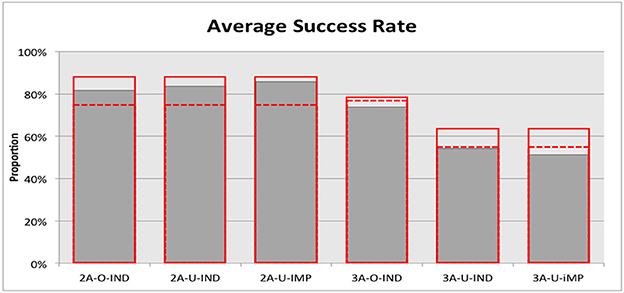
Figure 1. Average success rate. The red bars depict the theoretical predictions from the optimal, literally vague equilibria. The red dotted lines depict the predictions from the counterfactual in which Bob is constrained to be context independent.

Second, there was no significant difference in the success rates between Treatment 2A-U-IND and Treatment 2A-U-IMP (83.6 vs. 85.7%, two-sided Mann-Whitney test, p = 0.5192) and between Treatment 3A-U-IND and Treatment 3A-U-IMP (54.2 vs. 51.2%, two-sided Mann-Whitney test, p = 0.4897). This observation is also consistent with Hypothesis 1 that the imperativeness of Bob's message does not affect the success rate, regardless of the number of available actions. We thus have our first finding as follows:

Findings 1. Observability of Alice's message to Charlie affected the success rate only in the treatments with three actions. The imperativeness of Bob's message did not affect the success rate regardless of the number of available actions.

Figure 1 seems to suggest that the success rates observed in the three treatments with two actions (hereafter, Treatments 2A) are better approximated by the predictions from the optimal, context-dependent equilibrium languages than by the predictions from the context-independent counterfactual. Indeed, we cannot reject the null hypothesis that the success rates are not different from 87.5%, the predicted value from the optimal equilibrium (two-sided Mann-Whitney tests, p-values are 0.6325, 0.1509, 1 for Treatments 2A-O-IND, 2A-U-IND and 2A-U-IMP, respectively). Moreover, we can accept the alternative hypothesis that the success rates are significantly (Treatments 2A-U-IND and 2A-U-IMP) or marginally (Treatment 2A-O-IND) higher than the predicted level of 75% from the context-independent counterfactual (one-sided Mann-Whitney tests, p-values are 0.07571, 0.0004021, 0.0361 for Treatments 2A-O-IND, 2A-U-IND, and 2A-U-IMP, respectively), suggesting that the optimal, context-dependent equilibrium is a good predictor of the results observed from these treatments.

On the other hand, we do not receive the same observation from the three treatments with three actions (hereafter, Treatments 3A), especially those with unobservable messages from Alice. For Treatment 3A-U-IND, we cannot reject the null hypothesis that the success rate observed is the same as the success rate predicted by the context-independent counterfactual (two-sided Mann-Whitney tests, p = 1). Moreover, the success rates observed in Treatments 3A-O-IND was 73.8% and that in Treatment 3A-U-IMP was 51.2%, both strictly and significantly lower than the success rates predicted by the context-independent counterfactual (one-sided Mann-Whitney tests, p-values are 0.03574 and 0.0361, respectively). The non-parametric analysis suggests that the context-independent counterfactual is a better predictor of the results from Treatments 3A. Thus, we have the following result:

Findings 2. The average success rates observed in Treatments 2A-O-IND, 2A-U-IND, and 2A-U-IMP were significantly or marginally higher than the predicted level from the counterfactual in which Bob is context independent. The average success rates observed in Treatments 3A-O-IND, 3A-U-IND, and 3A-U-IMP were either not statistically different from or lower than the predicted level from the context-independent counterfactual.

Among Treatments 3A, more substantial deviations from the optimal, context-dependent equilibrium were observed in Treatments 3A-U-IND and 3A-U-IMP. This observed deviation in the average success rates may imply that context-dependent, literally vague languages did not emerge in those treatments, most likely due to the complexity of the environment considered. However, another completely plausible scenario would be that the observed deviation originates from a different source, such as Charlie's choices being inconsistent with the optimal equilibrium. Without taking a careful look at the individual behavior, it is impossible to draw any meaningful conclusions. Hence, in the subsequent sections, we look at individual players' choices.

4.2. Alice's behavior

Figure 2 reports Alice's message strategies by presenting the proportion of each message as a function of the number A, where data were grouped into bins by the realization of number A (e.g., [0, 5), [5, 10),..., etc.). Figure 2A provides the aggregated data from Treatments 2A, while Figure 2B provides the aggregated data from Treatments 3A. The same figures separately drawn for each treatment can be found in Appendix G.

FIGURE 2

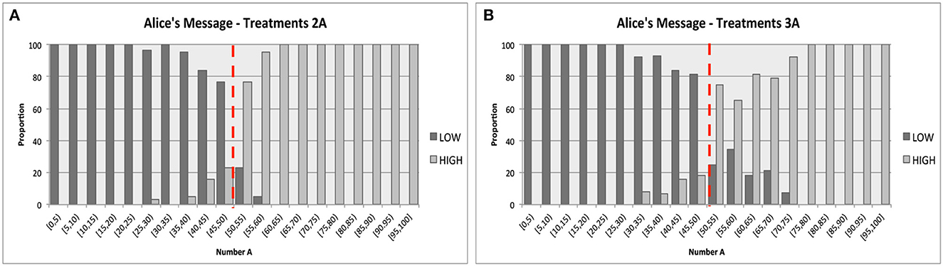
Figure 2. Alice's messages. The red dotted lines illustrate the optimal equilibrium strategy with a cutoff of 50. (A) Treatments 2A. (B) Treatments 3A.

From these two figures, it was immediately clear that the subjects with the designated role of Alice in our experiments tended to use cut-off strategies approximated well by the optimal cutoff of 50. Using the matching-group-level data from all rounds for each bin of the realized number A (e.g. [0, 5), [5, 10),..., etc.) as independent data points for each treatment, a set of (two-sided) Mann-Whitney tests reveals that 1) for any bins of A below 50, we cannot reject the null hypothesis that the proportion of message “A is Low” being sent was 100%, and 2) for any bins of A above 50, we cannot reject the null hypothesis that the proportion of message “A is Low” being sent was 0%. Among 20 bins in each treatment, the p-values for 14–17 bins were 1.0, while the lowest p-value for each treatment ranged between 0.2636 and 0.5637. We have the following result:

Findings 3. For any treatment, P_Alice(“Low”|A) = 1 for any A < 50 and P_Alice(“High”|A) = 1 for any A > 50.

The elicited strategies and beliefs reported in Figure 10 in Appendix C provided additional support for Finding 3. We cannot reject the null hypothesis that the reported cutoff values for Alice's strategy and other players' reported beliefs for Alice's strategy in all treatments were the same as the optimal equilibrium cutoff of 50 (two-sided Mann-Whitney tests, p-values range between 0.4533 and 1.000).

4.3. Bob's behavior

We now examine Bob's behavior. Recall that $P_{Bob}^L(m|B)$ denotes the proportion of Bob's message m given the realized number B and Alice's message “A is Low,” and $P_{Bob}^H(m|B)$ denotes the proportion of Bob's message m given Alice's message “A is High.” We introduced the measure of context dependence as $CD(B)=P_{Bob}^L(\overline{m}|B)-P_{Bob}^H(\overline{m}|B)$ where $\overline{m}$ is “B is Low” for the treatments with indicative messages and “Take DOWN” for the treatments with imperative messages. Figures 3A–F illustrate the distributions of CD(B) over the realization of number B, aggregated across all matching groups for each treatment. Again, the data from all rounds were grouped into bins by the realization of number B (e.g., [0, 5), [5, 10),..., etc.).

FIGURE 3

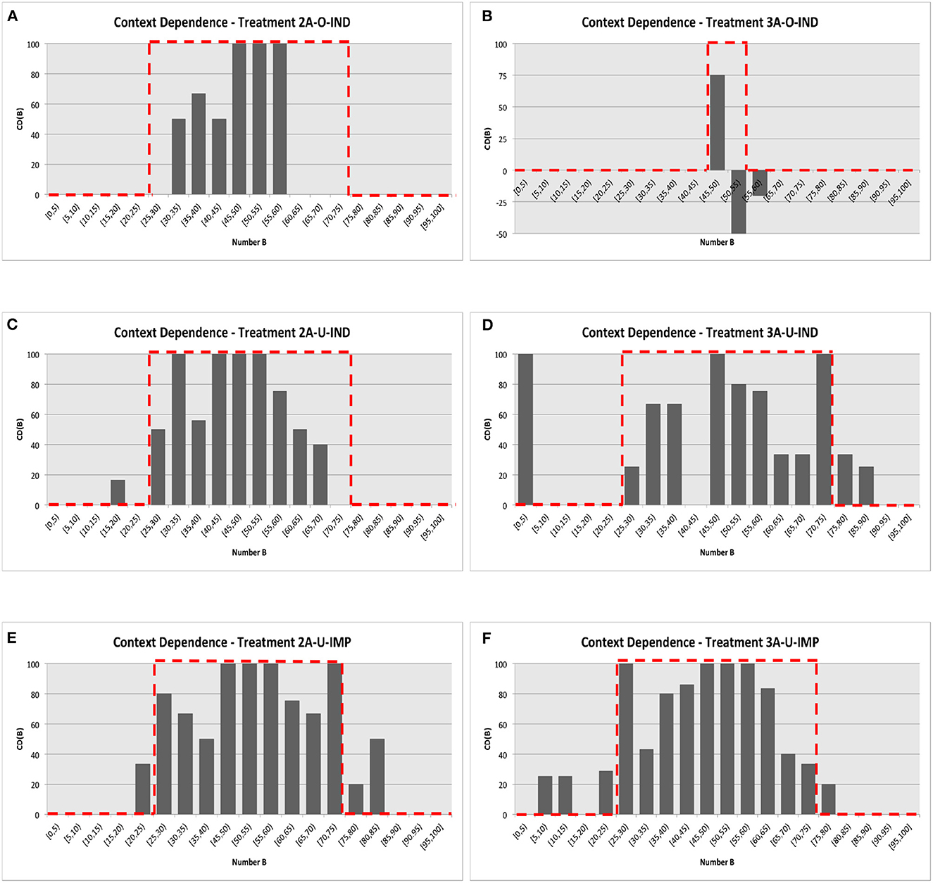
Figure 3. Bob's message strategy. The red dotted lines present the predicted distribution from the optimal equilibrium strategy. (A) Treatment 2A-O-IND. (B) Treatment 3A-O-IND. (C) Treatment 2A-U-IND. (D) Treatment 3A-U-IND. (E) Treatment 2A-U-IMP. (F) Treatment 3A-U-IMP.

The optimal, context-dependent equilibrium language implies that there exists an interval (strictly interior of the support of B) such that the value of CD(B) is 1 if B is in the interval and 0 otherwise. Moreover, the boundaries of such intervals are determined by the equilibrium cutoff strategy so that the interval is narrower in Treatment 3A-O-IND. The exact prediction of the distribution of CD(B) made by the optimal equilibrium is illustrated by the red-dotted lines in Figures 3A–F.¹⁷

These figures convincingly visualize the fact that, in each treatment, there exists an interval in which the value of CD(B) is strictly positive. For Treatment 2A-O-IND, for instance, we cannot reject the null hypothesis that CD(B) = 0 for B ∈ [0, 30) and for B ∈ [60, 100] (two-sided Mann-Whitney test, both p = 1.00). However, for B ∈ [30, 60), we can reject the null hypothesis that CD(B) = 0 in favor of the alternative that CD(B) > 0 (one-sided Mann-Whitney test, p = 0.04).¹⁸ Similarly, for Treatments 2A-U-IMP and 3A-U-IMP, we cannot reject the null hypothesis that CD(B) = 0 for the intervals of [25, 75) (p-values are 0.052 and 0.059, respectively) in favor of the alternative that CD(B) > 0. Qualitatively similar but less significant results were obtained from Treatment 2A-U-IND with the non-zero interval of [25, 70) (p = 0.136) and from Treatment 3A-U-IND with the non-zero interval of [25, 75) (p = 0.121). Thus, we have the following result:

Findings 4. In Treatments 2A-O-IND, 2A-U-IMP, and 3A-U-IMP, there existed an interval [X, Y] with X>0 and Y < 100 such that CD(B) > 0 if B ∈ [X, Y] and CD(B) = 0 otherwise.

We must discuss the data from Treatment 3A-O-IND in Figure 3B more carefully. First, as predicted by the optimal equilibrium strategy, the interval that has a non-zero value of CD(B) seemed to shrink significantly compared to any other treatments. Indeed, we cannot reject the null hypothesis that CD(B) = 0 for B ∈ [0, 45) and for B∈[50, 100] (two-sided Mann-Whitney test, p-values are 1.00 and 0.7237, respectively). However, a substantial deviation from the theoretical prediction was observed such that the reported value for the bin [50, 55) was negative.¹⁹ This observation was driven by the fact that the observed cutoff value from Bob's strategy conditional on Alice's message “A is Low” was 50, which may appear more focal than the theoretically optimal cutoff of 45.²⁰

The elicited strategies and beliefs reported in Figure 11 in Appendix C provide further supporting evidence. Wilcoxon signed-rank tests reveal that the reported cutoff values given Alice's message “A is Low” were significantly higher than the cutoff values given Alice's message “A is High” for most of the treatments (p-values ranged between 0.0004 and 0.0204) except for Treatment 3A-O-IND and Treatment 3A-U-IND.²¹ The fact that the reported cutoff values in Treatment 3A-O-IND were not significantly different (two-sided, p = 0.1924) is not surprising at all because the optimal equilibrium cutoff values are 45 and 55, distinctively more similar to each other than the predicted values for all other treatments. The insignificant result for Treatment 3A-U-IND (two-sided, p = 0.3561) originated mainly from two observations that the reported cutoffs from two Charlie subjects were 50 and 45 given “A is Low” and 85 and 80 given “A is High.”

4.4. Charlie's behavior

Figure 4 reports Charlie's action choices by presenting the proportion of each action as a function of information available to Charlie. Figure 4A presents the data aggregated across all matching groups of Treatments 2A, while Figure 4B presents the data aggregated across all matching groups of Treatments 3A.

FIGURE 4

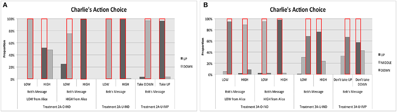
Figure 4. Charlie's actions. The red bars present the theoretical predictions from the optimal equilibria. (A) Treatments 2A. (B) Treatments 3A.

A few observations emerged immediately from these figures. First, Figure 4A reveals that observed strategy by Charlie depended to a limited extent on whether Alice's messages were observable to him in Treatments 2A. In Treatment 2A-O-IND, the proportion of UP that was chosen given Bob's message “B is High” was about 52% and the proportion of DOWN that was chosen given Bob's message “B is Low” was about 75%; both findings are substantially and significantly different from 100% predicted by the optimal equilibrium. However, the observed proportions become 63% and 100% if we take the last three rounds of data only, showing that learning took place in the right direction.²²

Second, Figure 4B reveals that MIDDLE was taken by Charlie in Treatment 3A-O-IND when the messages from Alice and Bob did not coincide. The proportions of MIDDLE that were chosen by Charlie given the message combinations (“A is High,” “B is Low”) and (“A is Low,” “B is High”) were higher than 90%. However, inconsistent with the prediction from the optimal equilibrium strategy, MIDDLE was taken even in Treatments 3A-U-IND and 3A-U-IMP. The proportions of MIDDLE that were taken in these two treatments varied between 24 and 43%, which are substantially larger than 0%. This observed deviation seemed persistent because it did not disappear even when we took the data from the last three rounds only.²³ Thus, we have the following result:

Findings 5. The modal action chosen by Charlie in all treatments are consistent with the predictions from the equilibrium with optimal, context-dependent language. More precisely,

• Charlie's observed action choices in Treatment 2A-O-IND were not the same as those observed in Treatment 2A-U-IND, showing that the observability of Alice's message to Charlie mattered.

• For Treatments 3A, MIDDLE was taken in Treatment 3A-O-IND when Charlie received different messages from Alice and Bob.

However, a substantial proportion of MIDDLE was observed even in Treatments 3A-U-IND and 3A-U-IMP.

This observed discrepancy in Charlie's action choices between our data and the prediction from the optimal equilibrium was the main source of the lower success rates we had in Treatments 3A-U-IND and 3A-U-IMP (see Figure 1). The success rates observed in Treatments 3A-U-IND and 3A-U-IMP were 54.2 and 51.2%, respectively, which are substantially lower than the predicted level of 63.5%, although the difference is statistically insignificant (Mann-Whitney tests, p-values are 0.4308 and 0.2413, respectively). If we replace Charlie's observed empirical choices with the hypothetical choices from the optimal strategy, the success rates in Treatments 3A-U-IND and 3A-U-IMP become 58.3% and 56.0%, respectively; both are substantially higher than the observed levels.

Note that MIDDLE was taken slightly more often in Treatment 3A-U-IMP than in Treatment 3A-U-IND (31 and 24% vs. 33 and 43%). The elicited strategies and beliefs presented in Figure 12 in Appendix C demonstrate this difference more vividly. This difference may originate from the fact that we framed Bob's messages as “Don't take UP” and “Don't take DOWN” to impose imperativeness to the messages for Treatment 3A-U-IMP.

4.5. Emergence of context-dependent, literally vague, and languages

In this section, we combine our findings presented in the previous sections to establish the emergence of context-dependent, literally vague languages. Admittedly, we did not present a perfect match between our data and the prediction from the optimal, context-dependent equilibrium language especially in the treatments with three actions. However, we provided convincing evidence that overall behavior observed in our laboratory was qualitatively consistent with the prediction at least in the treatments with two actions. More precisely,

1. Findings 1 and 2 presented that the overall outcome of each of the treatments with two actions was qualitatively consistent with the predictions form the equilibrium with the optimal, context-dependent language.

2. Finding 3 illustrated that Alice tended to use cut-off strategies approximated well by the cut-off value of 50 in all treatments. Thus, the contexts are properly defined.

3. Finding 4 showed that Bob tended to use context-dependent strategies at least in Treatments 2A-O-IND, 2A-U-IMP, and 3A-U-IMP.

4. Finding 5 suggested that Charlie understood the messages from the speaker(s) well and took actions in a manner that is qualitatively consistent with the optimal equilibrium strategy in all treatments.

5. Finding 5 also revealed that the lower success rates observed in Treatments 3A-U-IND and 3A-U-IMP reported in Finding 2 were driven largely by Charlie's behavior being partially inconsistent with the theoretical predictions from the optimal equilibrium.

Taking these findings together, we establish the following result:

Findings 6. The ways language was used by the speakers and understood by the listener were qualitatively consistent with the prediction from the optimal equilibria of the communication games especially when the strategic environment is simple. When the strategic environment is more complex, we observed more deviations from the prediction from the optimal equilibria.

5. Related literature

Economists have studied strategic language use since the cheap talk model was proposed by Crawford and Sobel (1982). Despite the formidable literature since generated on this subject, only recently was linguistic vagueness given the academic attention it deserves when Lipman (2009), asking “why is language vague”, defined vagueness and showed that vagueness has no advantage in the standard cheap talk setting with a common interest. In this line, Blume and Board (2013) explore a situation in which the linguistic competence of some conversing parties is unknown and show that this uncertainty could make the optimal language vague. The same authors further investigate the effect of higher-order uncertainty about linguistic ability on communication in Blume and Board (2014a) and find that in the common interest case, vagueness persists but efficiency loss due to higher-order uncertainty is small. Lambie-Hanson and Parameswaran (2015) study a model in which the listener may have a limited ability to interpret messages, and the sender may or may not be aware of this. The authors find that the optimal language can be vague. In Section 2, particularly by Examples 2, 3, we show that these models that enrich the simplest cheap talk can be unified and incorporated in our model by taking the meta-conversational uncertainty as the context dimension of the state. Our Proposition 1, while technically different from their findings, resonates the same keynote.

It is well known that even in the presence of a conflict of interest, endogenous vague language still has no efficiency advantage in the cheap talk framework. However, Blume et al. (2007) show that exogenous noise in communication, which forces vagueness upon the language, can generate a Pareto improvement. Blume and Board (2014b) further confirm that the speaker may intentionally exploit the noise to introduce more vagueness in the language. These papers differ from ours in that we focus on the common interest environment, and moreover, we study the efficiency foundation of endogenous vagueness.

Outside the field of economics, Lewis (1969) is a seminal philosophic analysis of language on this subject. Keefe and Smith (1997) and Keefe (2007) present extensive philosophical discussion on vague language, particularly vague language that gives rise to the Sorites paradox. van Deemter (2010) finds that in the field of computer science, vague instruction may make a search process more efficient than precise instruction.

On the experimental side, several recent papers investigate how the availability of vague messages improves or preserves efficiency. Serra-Garcia et al. (2011) show that vague language helps players preserve efficiency in a two-player sequential-move public goods game with asymmetric information. Wood (2022) explores the efficiency-enhancing role of vague language in a discretized version of canonical sender-receiver games à la Crawford and Sobel (1982). Agranov and Schotter (2012) show that vague messages are useful in concealing conflict between a sender and a receiver that, if it is publicly known, would prevent the parties from coordinating and achieving an efficient outcome. All these papers take the availability of vague messages as given and study how it affects players' coordination behavior. In contrast, we explore how a message endogenously obtains its vague meaning. For a more comprehensive discussion of the experimental literature on vague language, see the recent survey by Blume et al. (2020).

6. Concluding remarks

In this paper, we introduce the notion of context-dependence and literal vagueness, and offer our explanation of why language is vague. We show that literal vagueness arises in the optimal equilibria in many standard conversational situations. Our experimental data provide supporting evidence for the emergence of literally vague languages especially when the strategic environment is simple.

We would like to point out a few limitations to our study and where to go from here. First, one of the important premises in our analysis is that language is coarse: there are just not enough words to say everything in every detail, and hence a trade-off between precision and efficiency arises. In reality, vagueness could be present even when, theoretically speaking, the available vocabulary is sufficiently rich. In these cases, factors we leave out of our model, for instance the intrinsic cost/benefit of using each word, may be at play. Hence we do not consider context-dependence as the only explanation of vagueness. It would be interesting to theoretically and experimentally explore these other factors.²⁴ Second, although our discussion of linguistic vagueness focuses on an environment in which players' preferences are perfectly aligned, the theoretical discussions presented in Blume et al. (2007) and Blume and Board (2014b) suggest that the communicative advantage of literal vagueness would be extended to an environment with conflicts of interest. We believe that experimentally investigating the role of vagueness in the presence of conflicts of interest is an interesting avenue for future research.

Author contributions

Both authors listed have made a substantial, direct, and intellectual contribution to the work and approved it for publication.

Funding

This study was supported by a grant from the Research Grants Council of Hong Kong (Grant No. GRF-16502015). The open access publication fees will be paid by the internal funding provided by the Department of Economics at HKUST.

Acknowledgments

We are grateful to Andreas Blume, Itzhak Gilboa, Ke Liu, Joel Sobel, and Alistair Wilson for their valuable comments and suggestions. For helpful comments and discussions, we thank seminar and conference participants at the SURE International Workshop on Experimental and Behavioral Economics (Seoul National University). Hanyu Xiao provided excellent research assistance.

Conflict of interest

The authors declare that the research was conducted in the absence of any commercial or financial relationships that could be construed as a potential conflict of interest.

Publisher's note

All claims expressed in this article are solely those of the authors and do not necessarily represent those of their affiliated organizations, or those of the publisher, the editors and the reviewers. Any product that may be evaluated in this article, or claim that may be made by its manufacturer, is not guaranteed or endorsed by the publisher.

Supplementary material

The Supplementary Material for this article can be found online at: https://www.frontiersin.org/articles/10.3389/frbhe.2023.1014233/full#supplementary-material

Footnotes

1. ^The formal game-theoretic version of this definition is first given in Lipman (2009).

2. ^The linguistic literature has identified context dependence as a factor that could be connected to vagueness (e.g., Mills, 2004), although the linguistic approach is quite different from an economic one. Here, what we do is providing an explanation for vagueness in terms of context dependence in a formal, game-theoretic model of communication.

3. ^This model, particularly the common interest assumption, follows Lipman (2009). When there is a conflict of interest, the role of vagueness as an efficiency-enhancing device is well understood in the literature (see, e.g., Blume et al. 2007; Blume and Board 2014b).

4. ^The notions of context and literal vagueness in our framework resemble the “prior collateral information” in Quine (1960) and the “indeterminacy of indicative meaning” of Blume and Board (2013), respectively. Example 2 and its subsequent discussion further elaborate how one can relate our discussion of literal vagueness to that provided by Blume and Board (2013). For additional discussion, see the literature review in Section 5.

5. ^It is not uncommon in the literature to consider a limited number of messages available for communication. For example, Sobel (2015) takes a common-interest version of Crawford and Sobel (1982) and investigates how the number of available messages shapes the optimal language. Similarly, Cremer et al. (2007) study optimal codes within firms when the set of words is finite. For a more recent discussion, see Dilmé (2017), who covers the limit case of both Sobel (2015) and Cremer et al. (2007).

6. ^This notion is related to the indirect speech act in linguistics. Speaking directly about context when answering a question only about features may be awkward and is thus more costly. The degree of awkwardness an individual feels may differ, and those who feel more awkward may use only vague language. For more details, see Pinker (2007).

7. ^The prefix “meta-” means “on a higher level”.

8. ^We do not instead compute the fraction of preferences satisfying U1-U3 among all preferences because preferences with indifference compose a majority of all preferences when the number of alternatives is large, despite that utility functions with indifference are only measure zero.

9. ^A similar categorization of equilibria persists for variations of the benchmark game to be introduced. For those variations, we will skip the analysis of equilibria in which a converser babbles because they are of no theoretical consequence and do not correspond to the experiment results.

10. ^Of course, there are outcome-equivalent equilibria in which Bob uses the messages in the opposite way. We do not explicitly itemize such equilibria here and thereafter.

11. ^The key logic is that Alice would use a cutoff of 50 because of the problem's symmetry. Thereafter, the optimal cutoffs of 25 and 75 can be deduced in one's head or at most in a back-of-envelope calculation.

12. ^For example, Bob's message spaces in Treatments 2A-U-IND and 2A-U-IMP are {“B is HIGH,” “B is LOW”} and {“Take UP,” “Take DOWN”}, respectively.

13. ^Charlie's optimal strategy remains the same regardless of whether Bob is constrained to be context independent or not.

14. ^To make the likelihood of each action being ideal exactly equal across two actions, we set both actions to be ideal when A + B = 100.

15. ^Although we were aware that an appropriate incentive-compatible mechanism is needed to correctly elicit beliefs, we used this elicitation procedure because of its simplicity and the fact that the belief and strategy data were only secondary data used mainly for the robustness checks.

16. ^Under the Hong Kong currency board system, the Hong Kong dollar is pegged to the US dollar at the rate of HK $7.8 = US$1.

17. ^Figures 8A–F, 9A–F presented in Appendix C separately report the distributions of $P_{Bob}^L(\mathrm{\text{“}}B\mathrm{\text{ is Low”}}|B)$ and of $P_{Bob}^H(\mathrm{\text{“}}B\mathrm{\text{ is Low”}}|B)$ for each treatment.

18. ^To conduct Mann-Whitney tests for Hypothesis 4, we first eyeball Figures 3A–F to identify the plausible choices of the interval with CD(B) > 0 for each treatment. For example, for Treatment 2A-O-IND, relying on Figure 3A, we divide the support of number B into three intervals—[0, 30), [30, 60), and [60, 100]. We next calculate the value of CD(B) for each of the three intervals for each matching group. Taking those values as group-level independent data points for each treatment, we conducted the non-parametric test.

19. ^For Treatment 3A-O-IND, we cannot conduct any meaningful statistical analysis for B ∈ [45, 50) because there are only two group-level independent data points.

20. ^Similarly, two substantial deviations were observed in Treatment 3A-U-IND - in the first bin of [0, 5) and the ninth bin of [40, 45) in Figure 3D. The first deviation was driven solely by the single data point with B ∈ [0, 5) in which Bob sent “B is High” after receiving “A is High” from Alice. The second deviation was driven solely by the single data point with B ∈ [40, 45) in which Bob sent “B is Low” after receiving “A is High” from Alice.

21. ^To conduct Wilcoxon signed-rank tests, we pooled the data from the reported cutoff values for Bob's strategy and other players' reported beliefs.

22. ^In an early stage of the project, we conducted two sessions in which subjects participated in the first 20 rounds with the treatment condition of 2A-U-IND and in the second 20 rounds with the treatment condition of 2A-O-IND. The data from the second 20 rounds were almost perfectly consistent with the theoretical prediction, showing convincing evidence of learning. Data from this additional treatment are available upon request.

23. ^The elicited strategies and beliefs presented in Figure 12 in Appendix C were highly consistent with the results in Finding 5.

24. ^A recent paper along this dimension is Suzuki (2021).

References

Agranov, M., Schotter, A. (2012). Ignorance is bliss: an experimental study of the use of ambiguity and vagueness in the coordination games with asymmetric payoffs. Am. Econ. J. Microecon. 4, 77–103. doi: 10.1257/mic.4.2.77

CrossRef Full Text | Google Scholar

Blume, A., Board, O. (2013). Language barriers. Econometrica 81, 781–812. doi: 10.3982/ECTA9183

CrossRef Full Text | Google Scholar

Blume, A., Board, O. (2014a). “Higher-order uncertainty about language,” in Working Paper.

Google Scholar

Blume, A., Board, O. (2014b). Intentional vagueness. Erkenntnis 79, 855–899. doi: 10.1007/s10670-013-9468-x

CrossRef Full Text | Google Scholar

Blume, A., Board, O. J., Kawamura, K. (2007). Noisy talk. Theor. Econ. 2, 395–440.

Google Scholar

Blume, A., Lai, E. K., Lim, W. (2020). “Strategic information transmission: A survey of experiments and theoretical foundations,” in Handbook of Experimental Game Theory, eds C. Monica Capra, R. Croson, M. Rigdon, and T. Rosenblat (Cheltenham; Northampton, MA: Edward Elgar Publishing).

Google Scholar

Crawford, V., Sobel, J. (1982). Strategic information transmission. Econometrica 50, 1431–1451. doi: 10.2307/1913390

CrossRef Full Text | Google Scholar

Cremer, J., Garicano, L., Prat, A. (2007). Language and the theory of the firm. Q. J. Econ. 122, 373–407. doi: 10.1162/qjec.122.1.373

CrossRef Full Text | Google Scholar

Dilmé, F. (2017). “Optimal languages,” in Working Paper.

Google Scholar

Fischbacher, U. (2007). z-tree: Zurich toolbox for ready-made economic experiments. Exp. Econ. 10, 171–178. doi: 10.1007/s10683-006-9159-4

CrossRef Full Text | Google Scholar

Keefe, R. (2007). Theories of Vagueness. Cambridge Studies in Philosophy. Cambridge: Cambridge University Press.

Google Scholar

Keefe, R., Smith, P. (1997). Vagueness: A Reader. Cambridge, CA: MIT Press.

Google Scholar

Lambie-Hanson, T., Parameswaran, G. (2015). A Model of Vague Communication. Mimieo.

Google Scholar

Lewis, D. (1969). Convention: A Philosophical Study. Cambridge, MA: Harvard University Press.

Google Scholar

Lipman, B. L. (2009). “Why is language vague,” in Working Paper.

Google Scholar

Mills, E. (2004). Williamson on vagueness and context-dependence. Philos. Phenomenol. Res. 68, 635–641. doi: 10.1111/j.1933-1592.2004.tb00370.x

CrossRef Full Text | Google Scholar

Pinker, S. (2007). The Stuff of Thought: Language as a Window Into Human Nature. Penguin.

PubMed Abstract | Google Scholar

Quine, W. V. O. (1960). Word and Object. Cambridge: Technology Press of the Massachusetts Institute of Technology.

Google Scholar

Serra-Garcia, M., van Damme, E., Potters, J. (2011). Hiding an inconvenient truth: lies and vagueness. Games Econ. Behav. 73, 244–261. doi: 10.1016/j.geb.2011.01.007

CrossRef Full Text | Google Scholar

Sobel, J. (2015). “Broad terms and organizational codes,” in Working Paper.

Google Scholar

Suzuki, T. (2021). Pragmatic Ambiguity and Rational Miscommunication. University of Technology Sydney. Available online at: https://www.uts.edu.au/sites/default/files/article/downloads/Working%20paper_SUZUKI%20Toru.pdf

Google Scholar

van Deemter, K. (2010). Vagueness Facilitates Search. Berlin; Heidelberg: Springer Berlin Heidelberg.

Google Scholar

Wood, D. H. (2022). Communication-enhancing vagueness. Games 13, 49. doi: 10.3390/g13040049

CrossRef Full Text | Google Scholar