
94% of researchers rate our articles as excellent or good
Learn more about the work of our research integrity team to safeguard the quality of each article we publish.
Find out more
METHODS article
Front. Bee Sci. , 09 February 2024
Sec. Bee Protection and Health
Volume 2 - 2024 | https://doi.org/10.3389/frbee.2024.1329844
This article is part of the Research Topic Horizons in Bee Science View all 10 articles
 André Luis Acosta1,2*†
 Charles Fernando dos Santos3†
 Vera Lucia Imperatriz-Fonseca1,2,4†Ricardo Caliari Oliveira5†
 Tereza Cristina Giannini2,6†
Climate change is affecting wild populations worldwide, and assessing the impacts on these populations is essential for effective conservation planning. The integration of advanced analytical techniques holds promise in furnishing detailed, spatially explicit information on climate change impacts on wild populations, providing fine-grained metrics on current environmental quality levels and trends of changes induced by estimated climate change scenarios. Here, we propose a framework that integrates three advanced approaches aiming to designate the most representative zones for long-term monitoring, considering different scenarios of climate change: Species Distribution Modeling (SDM), Geospatial Principal Component Analysis (GPCA) and Generalized Procrustes Analysis (GPA). We tested our framework with a climatically sensible Neotropical stingless bee species as study case, Melipona (Melikerria) fasciculata Smith, 1854. We used the SDM to determine the climatically persistent suitable areas for species, i.e. areas where the climate is suitable for species today and in all future scenarios considered. By using a GPCA as a zoning approach, we sliced the persistent suitable area into belts based on the variability of extremes and averages of meaningful climate variables. Subsequently, we measured, analyzed, and described the climatic variability and trends (toward future changes) in each belt by applying GPA approach. Our results showed that the framework adds significant analytical advantages for priority area selection for population monitoring. Most importantly, it allows a robust discrimination of areas where climate change will exert greater-to-lower impacts on the species. We showed that our results provide superior geospatial design, qualification, and quantification of climate change effects than currently used SDM-only approaches. These improvements increase assertiveness and precision in determining priority areas, reflecting in better decision-making for conservation and restoration.
Climate change and biodiversity loss are two major environmental challenges facing the planet. Studies have shown that the current climate crisis is already affecting the physiologies, genomes, distributions, interactions, and behaviors of many wild species, including bees (Kerr et al., 2015; Hegland et al., 2021; Barbosa et al., 2022; Schonfeldt et al., 2022; Sgolastra et al., 2022). These changes are expected to worsen in the coming decades, with significant implications for species survival and ecosystem functioning (IPCC-AR6, 2021). To address the urgent need for effective conservation strategies in the face of climate change crisis, new integrative approaches are required (Foden et al., 2018).
Species Distribution Modeling is an effective approach used to evaluate both the present status and future scenarios of potential changes in climate suitability for species, especially in the context of climate change. This analytical method can play a crucial role in aiding decision-making processes for biodiversity restoration and conservation (Kearney et al., 2010; Ferraz et al., 2012; Guisan et al., 2013; Angelieri et al., 2016; Sofaer et al., 2019). Climate suitable areas represent sites that are most adequate for the occurrence of species in different climate scenarios. Combined with Geographic Information System, they also can provide straightforward and intuitive graphical representations of possible trends of change for species and areas, facilitating the visualization and interpretation of the effects of climate change in temporal and spatial dimensions (Kearney et al., 2010; Ferraz et al., 2012; Guisan et al., 2013; Angelieri et al., 2016; Sofaer et al., 2019). SDM relies on the relationship between environmental variables and empirical data on the target-species occurrence. The most relevant ranges and composition of environmental factors in explaining species occurrence are quantified and mapped, generating a baseline scenario (Diniz-Filho et al., 2009; Espíndola and Pliscoff, 2018; Hao et al., 2019; Huang et al., 2022; Marshall et al., 2023). Subsequently, the characteristics detected in the baseline scenario are then projected on a new set of variables with predicted variations for future climate change scenarios (Hulme, 2005; Ludena and Yoon, 2015; Li et al., 2018). This projection enables the identification of areas that will suffer different changes in the climate suitability for the species. It is plausible to expect that greater changes will impose greater climate pressure on populations, and these areas can be defined as priorities for actions aimed at mitigating the impacts of climate change. Equally important are the currently climatically suitable areas that will suffer milder impacts in the future, as they are essential for the conservation of the species, safeguarding the species for future. Therefore, areas that are suitable for species today and will continue to be suitable in the future are targeted for this approach. Here, we call this zone as Persistent Suitable Extent (PSE), which are contiguous regions that will consistently offer a suitable climate for species survival from the present into the future, and can function as potential sanctuaries, since adverse effects of climate change in populations are less intense, potentially allowing the maintenance of the populations. Therefore, the PSE are of great interest for long-term monitoring and status assessments, as well as, priority zones for land cover restoration and conservation planning (Hulme, 2005; Ludena and Yoon, 2015; Li et al., 2018).
The Generalized Procrustes Analysis (GPA) is a multivariate analysis used for comparing the concordance (and discordance) among a set of matrices (Gower, 1975; Dijksterhuis and Gower, 1991; Goodall, 1991; Ren et al., 2016; Cheng et al., 2021). For example, it has been frequently used for studies on morphological shapes (Rohlf, 1998; Nicola et al., 2003; Mitteroecker and Gunz, 2009; Viscosi and Cardini, 2011; Klingenberg, 2016; dos Santos et al., 2019). But it can also be employed as sensory analysis (Risvik et al., 1994; Mauricio et al., 2016; Ser, 2019; Rodríguez-Noriega et al., 2021), ecology (Lisboa et al., 2014; Camiz et al., 2017) and genetics (Bramardi et al., 2005; Xiong et al., 2008a). GPA is obtained after Procrustes transformation, defined as translation, rotation, reflection, and isotropic scaling (Gower, 1975; Ten Berge, 1977; Dijksterhuis and Gower, 1991; Goodall, 1991; Risvik et al., 1994). In short, translation means that all individual configurations are displaced to the center of the projective mapping, while they are rotated and reflected for an optimal agreement with one another. Yet, isotropic scaling is concerned to shrinking/stretching of individual configurations in a way that they are, as much as possible, alike to one another while relative distances among objects are preserved (Gower, 1975; Ten Berge, 1977; Dijksterhuis and Gower, 1991; Goodall, 1991; Risvik et al., 1994). Thus, GPA has two relevant attributes: it is based on a consensus configuration that is projected in a multidimensional space and it allows calculating the level of within-variance of each assessed item. Therefore, according to environmental matrices extracted from climate variables into the persistent suitability area delimitated by the suitability models, GPA inform the level and direction of potential convergences among scenarios. In addition, since the persistent suitability area of the target organism was sliced in a set of inner regions by a Geospatial Principal Component Analysis (GPCA) zoning approach (please do not confuse with Generalized PCA; see details in Material and Methods), the GPA analysis is able to indicate inner regions where all combined variables are prone to a greater within-variation, indicating were populations may face a higher climatic pressure. Conversely, regions within climatic suitability would exhibit lower within-variation, indicating places under lower climatic disturbance, therefore, populations under lower pressure. Such sites are considered as priority areas for long-term ecological, genetic or morphological studies, but also contributes to decision-making on the prioritization of areas for assessments, monitoring, restoration and conservation planning, as these locations can function as potential wildlife sanctuaries for many species in the future, and help guarantee the essential conditions for the existence or reproduction of resident and migratory fauna.
We relied on a native Brazilian stingless bee species to test our framework, the stingless bee Melipona (Melikerria) fasciculata Smith, 1854. Bees play the major pollinator role, providing several ecological, economic and social benefits, with significant impact in nature conservation, in agriculture and human societies (Klein et al., 2007; Potts et al., 2010; Ollerton et al., 2011; Chaplin-Kramer et al., 2014; Potts et al., 2016; Hristov et al., 2020; Klein et al., 2020; Patel et al., 2020). The stingless bees are the most diverse group of social bees and are found in the tropical and subtropical regions of the world, comprising more than 605 described species (Moure et al., 2022; Engel et al., 2023; Roubik, 2023). Several stingless bee species are traditionally managed by human populations around the world having not only economic but cultural importance (Cortopassi-Laurino et al., 2006; Quezada-Euán et al., 2018; Hill et al., 2019). Melipona fasciculata is a prominent stingless bee species inhabiting natural areas within Amazon biome (northern Brazil), managed for honey production by people living therein (Jaffé et al., 2015; Venturieri et al., 2015; Farfan et al., 2022), playing a key role as pollinator of native plants in the forest and in cultivated plants requiring buzz-pollination (Maués and Couturier, 2002; Nunes-Silva et al., 2013; Giannini et al., 2015; Gostinski et al., 2018). Their foraging flight and homing capability has been estimated to cover large distances as 10 km (Nunes-Silva et al., 2020). M. fasciculata is one of the most studied and reared stingless bees in North Brazil (Venturieri et al., 2017).
Here, we propose a methodological framework that integrates three advanced analytical approaches to determine the most representative sampling areas for monitoring aimed at assessing ecological and molecular long-term effects of climate change on populations. Our framework aims to: (A) identify the persistent suitable extent for the species under climate change scenarios; (B) discriminate inner zones based on climatic variability inside the persistent suitable extent by applying GPCA analysis as a zoning approach and; (C) determine different levels of spatial and temporal climatic variability in each inner zone by applying GPA. We used a native stingless species to test our framework, but it can subsidies other studies aiming to prioritizing areas for planning actions and policies for restoration and environmental conservation to protect other species.
We collected empirical data for M. fasciculata occurrence from the following databases: (a) speciesLink biodiversity database (http://splink.org.br/); (b) Global Biodiversity Information Facility biodiversity database (GBIF, 2023; DOI: 10.15468/dl.gvxe6y); and a database resulted from recent fieldwork (Almeida, 2022). After an initial screening, we excluded records containing inaccurate coordinates (e.g. lacking numbers and signals), dubious positions (e.g. records over water/ocean) and repeated records with the same coordinates for the target species (database available in Supplementary Material 1).
The recent recommendations of IPCC report (IPCC-AR6, 2021) consolidated the Coupled Model Intercomparison Project (CMIP6) for as Global Circulation Models (GCM), which enhanced the accuracy of climate effect estimates, with substantial changes in emission trends and spatial distributions (Hausfather, 2019; Mcbride et al., 2021). Updated climatic variables, which have a direct effect on terrestrial species, suggest that climate suitability models for species must be either renewed or newly proposed to support accurate decisions (Mcbride et al., 2021; Schramek, 2021).
We retrieved three sets of digital layers representing 19 bioclimatic variables and altitude from Worldclim (Fick and Hijmans, 2017). These bioclimatic variables geographically express averages, seasonality, and extremes of precipitation and temperature, and combinations thereof. The first set is historical variables, representing interpolated empiric climatic conditions of the period 1970-2000. The other two sets are the most recent (CMIP6) Global Circulation Models (GCM) projections generated for future climate scenarios released by the Japanese Agency for Marine-Earth Science and Technology (GCM named MIROC6) according to the SSP585 scenarios. Each set represents the climate estimated for two upcoming periods, from 2021 to 2040 and from 2041 to 2060. Although they are represented as periods, these layers reflect the outcome of each scenario to be achieved at the end of each period. For practical purposes, the scenario periods will be referred to as the last year of each respective period: 2040 and 2060. Since M. fasciculata occurs only in the Brazilian territory, all the environmental variables were cropped for the Brazilian administrative extent (IBGE, 2022), and were used at the same geographical extension (Brazil) and high resolution (2.5 arc minutes).
Among the Shared Socioeconomic Pathways (SSP), the 5-8.5 is one of the most intensive global greenhouse gas emission trajectories estimated by the AR6 (IPCC-AR6, 2021). Although it is not possible to guarantee the consolidation of any scenario as the most likely climate of the future, this seems to be the most appropriate scenario for this study. We argue that more intense effects improves the approach’s discriminative capacity by detecting regions whose species will be under lower and higher climatic pressure. Additionally, future projections aiming to prioritize regions for monitoring and to define conservation areas must observe the worst possible scenario, so that the actions planned to safeguard species will be efficient in the future consolidation of any possible scenarios, including the pessimistic one. The set of 19 bioclimatic variables (baseline period from 1970 to 2000) was tested aiming to exclude variables with highest correlation between each other, which could compromise the predictive quality of the models from regression algorithms due to effect of multicollinearity. For this purpose, we applied the Variance Inflation Factor Analysis (vifcor function) from R package’s usdm (Naimi et al., 2014). Thereafter, we used the selected set of variables for the modeling procedure (see Supplementary Material 2).
To map the geographical shape of species climatic suitability for the species in the baseline conditions (1970-2000), we used a habitat suitability approach (Hirzel and Le Lay, 2008) by means of the SDM tool Biomod2 package version 3.5.1 (Thuiller et al., 2021) in R platform (R Core Team, 2021). We selected five Biomod2 algorithms: GLM – Generalized Linear Model (package glm: Hastie and Pregibon, 1992); GBM – Generalized Boosting Model (package gbm: Greenwell et al., 2020); GAM – Generalized Additive Model (package mgcv: Hastie and Tibshirani, 1990); RF – Random Forest (package randomForest: Breiman, 2001); MAXENT – Maximum Entropy (package maxent: Phillips et al., 2021). We chose these algorithms based on the results of Aguirre-Gutiérrez et al. (2013) and Acosta et al. (2016), who showed high performance for similar applications. We followed the parameterization of the algorithm as recommended by the authors (Guisan and Thuiller, 2005; Phillips et al., 2006; Thuiller et al., 2009; Thuiller et al., 2021).
In addition to the species presences, the modeling approach also requires data on absences. However, this type of data is rarely available, and for the targeted species, there is no confirmed geographic statement of absences. To fulfill this demand, five pseudo-absences datasets with 10 times the number of presences (based in Chefaoui and Lobo, 2008; for better predictive performance in similar modeling circumstances) were randomly generated outside the predefined geographic exclusion zones (20 km buffer radius) around the presences. These zones represent twice the distance species individuals could travel from their colonies throughout their lifetime (Nunes-Silva et al., 2020), and thus no pseudo-absences were assigned within them.
At each round of modeling, the set of presence points was randomly divided into 80% dedicated to model training, and 20% to evaluate the predictive quality by true skill statistics (TSS; Allouche et al., 2006). This random selection was replaced at each modeling run (RUN), in the same way that the pseudo absence datasets were also randomly replaced per round (PA). We then generated 125 models for M. fasciculata in the baseline climate scenario. This amount results from the combination of five algorithms, five randomly generated pseudo-absence datasets, and five random partitioning of the species presence datasets (5*5*5 = 125).
In the modeling framework, we only maintained the models with best predictive performance per species, which were evaluated by TSSs > 0.8 (evaluation data and selection in Supplementary Material 3). These selected models were used to build a baseline ensemble forecast model (BEFM) based on the Committee Averaging method. This method was defined as a conversion of probabilistic predictions from single models into binary predictions using a threshold maximizing specificity and sensitivity, and then averaging them (Wisz et al., 2008; Hao et al., 2019; Thuiller et al., 2021). The same set of mathematical models used to generate the BEFM, were also projected for future scenarios using Biomod2 projection function. Subsequently, each ensemble forecast model (baseline, 2040 and 2060) were reclassified as follows: zones showing suitability values >= 75% were converted into 1. The remaining areas, with < 0.75%, were converted into zero, meaning unsuitable for the species. The reason for classifying the continuous models into binary values is to geographically circumscribe four types of areas: A) currently climatically suitable area and that will remain suitable in the future (Figure 1A; Delta blue cell=11); B) currently climatically suitable area that will become unsuitable in the future (Figure 1A; Delta red cell=10); C) currently unsuitable area that will become climatically suitable in the future (Figure 1A; Delta green cell=01) and; D) areas always unsuitable to the species (Figure 1A; Delta white cell=00). For this, we used a geospatial overlay strategy of binary models to detect these four areas (see Figure 1A). After generating the delta models, which compare the baseline and each future scenario individually, we compared the both deltas generated by concatenating side-by-side binary values (Figure 1B). Only cells matching suitability in both future scenarios were determined as Persistent Suitable Extent (PSE; Figure 1B). Although areas showing loss of suitability may be of interest for wildlife monitoring, rescue and management, for our approach (oriented to long-term ecological and genetic studies) these areas were not targeted. Likewise, zones that maintained or gained suitability from the baseline to a single future scenario, but not in both futures, were also not considered.
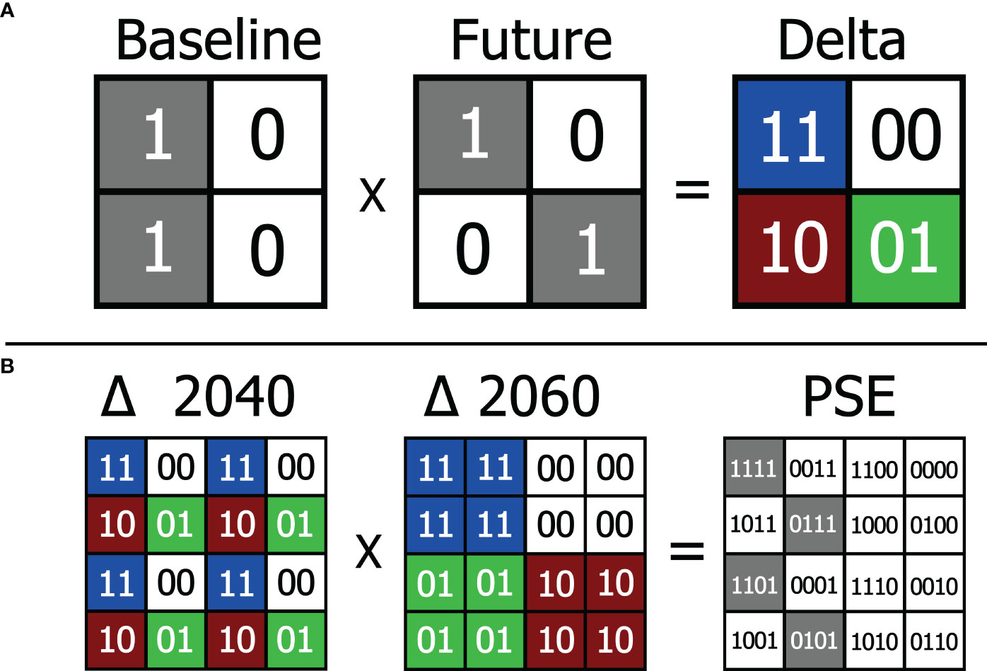
Figure 1 The upper part of the figure (section A) shows raster fragments of four cells from baseline and future EFMs, presenting values = 1 for areas suitable for the species and = 0 for areas unsuitable. Overlapping the baseline with the future fragment (e.g. 2040) we obtained the Delta Model, therefore the sum of the binary values generate four possible values: 11 for locations that will remain climatically suitable; 00 for locations that will remain unsuitable; 01 for unsuitable locations that will gain suitability and; 10 for locations that will lose suitability. At the bottom (section B) we have an example with 16 cells showing all possibilities of crossing between Deltas (2040 x 2060), obtaining a single combined result. For our study, only cells with suitability in both future scenarios (green and blue) were considered safe for long-term maintenance of the species, hence the extension we called persistent suitable zone (PSE; gray cells).
For better spatial discrimination of the zone with variable intensity (higher to lower) of climate change within the environmental range still suitable for the occurrence of the species today and in the both future scenarios (PSE), we divided it into 10 inner belts based on the current variability of climatic conditions. For that, we used Principal Component Analysis as an approach for the geographical zoning. Since our approach is a geographic space-oriented PCA, we refer to this analysis as Geospatial PCA; however, we emphasize that we are not dealing with Generalized PCA, but Geospatial PCA (GPCA). This approach has demonstrated to be very accessible, as it is present at almost all free geographic information system and programming platforms, and ideal for our purposes, as it can reduce the dimensionality of large data sets, increasing interpretability while minimizing the loss of information. This technique assesses multiple variables simultaneously and creates other variables, either reducing or nullifying the level of correlation among them and successively maximizing the variance, which is an aspect of great interest for this study (Gavioli et al., 2016; Jollife and Cadima, 2016).
This zoning approach aims to show climate variability along the extension of the persistent suitability area, aggregating into belts the climatically most similar areas in terms of climatic variation based on the thermal and precipitation extremes and averages. Thus, we will maximize the variability convergence within each belt and, simultaneously, maximize the variability divergence between each belt. Therefore, the climatic variability within belt 1 will be quite different from that found in belt 10, and although belt 1 differs from belt 2, it does so to a lesser level than in belt 10. This 10-zone gradient allows us to look at persistent suitability areas as ten climatically particular zones, and to compare them we applied the GPA.
As axes for the GPCA, we used a set of six variables in current condition from Worldclim (Fick and Hijmans, 2017), the ones that better represent the centrality and extremes of the thermal and rainfall amplitudes into the persistent suitability areas. They are Annual Mean Temperature (Bio 1); Maximum Temperature of Warmest Month (Bio 5); Minimum Temperature of Coldest Month (Bio 6); Annual Precipitation (Bio 12); Precipitation of Wettest Month (Bio 13); Precipitation of Driest Month (Bio 14).
Here, to determine de belts, we exclusively selected the eigenvalues from the first PCA axis (into GPCA), which often explain more than 50% of the total variance. The range of eigenvalues variation was normalized from 0 to 1, and subsequently, the value was partitioned into deciles, so that these ten ranges could represent spatial clippings that we call the GPCA Zones as PCAZ. Subsequently, we plotted and enumerated these PCAZ (from 1 to 10) for posterior identification. Therefore, the PCAZ 1 will always be the most divergent in variance with respect to the opposite extreme, the PCAZ 10, which does not necessarily imply linearity. The relevant climatic differences among PCAZ were later depicted in the GPA. We performed the Geospatial PCA (GPCA) approach by using the R software with the function rasterPCA from package RStoolbox v. 0.3.0 (Leutner, 2022). After the GPCA zoning, the climatic values from all respective six variables projected for both future scenarios (2040 and 2060) were also extracted to be further used in the Generalized Procrustean Analysis.
We performed the Generalized Procrustean Analyzes (GPA; Gower, 1975; Dijksterhuis and Gower, 1991) to assess the positioning, displacement (trajectories) and variability of bioclimatic factors (above mentioned), relating and comparing the three scenarios (baseline, 2040 and 2060), considering exclusively and individually the ten geospatially compartmentalized PCAZ into the persistent suitability areas.
GPA is particularly relevant for investigating the concordance among a set of matrices having as a baseline a consensus configuration projected in a multidimensional space, and it allows calculating the level of within-variance of each assessed item (Gower, 1975; Dijksterhuis and Gower, 1991). GPA was performed with the ‘GPA’ function in the package FactoMineR (Lê et al., 2008). The tolerance level for solution convergence was set to 100-10 and the number of iterations was set to 199. Then, we applied a permutation test with 99 permutations by means of the “GPA.test” function of the package RVAideMemoire (Hervé, 2020) to test whether both the bioclimatic variables and the zones were not positioned randomly in the GPA multidimensional spaces (Wakeling et al., 1992; Xiong et al., 2008a; Xiong et al., 2008b). Such a permutation test provides an observed Rc value that can be interpreted as the proportion of the original variance explained by the consensus configuration significantly higher than 95% of the results that are obtained when permuting the data (Xiong et al., 2008b).
We used two output metrics of the GPA, the bioclimatic similarity between future periods with the baseline scenario, and the size of the residuals (within-variance) of the bioclimatic variables and PCAZ. In the first case, similarity was extracted from the ‘Residual variance’ (RV) coefficients resulting from GPA outputs (Lê et al., 2008). RV coefficient varies from 0 to 1, values close to 1 would indicate scenarios more similar each other, while values closer to 0 would indicate higher discrepancy between scenarios. GPA output also generates the size of residual for each item investigated by minimizing the residual sum of squares between points and its underlying centroids corresponding n dimensions (Lisboa et al., 2014). Thus, the higher the residuals, the more the elements differ in terms of the consensus configuration. In fact, this suggests a poor fit and, consequently, a higher underlying variance that can be interpreted as having higher within-discrepancies (Lisboa et al., 2014). As result, we labeled the bioclimatic variables and/or zones as more or less congruent according to how concordant (small or negligible residuals) or discordant (greater residuals) they were following the GPA. That is, one might expect a higher ecological pressure on the populations of M. fasciculata if there are large discrepancies among all bioclimatic variables within the zones, which may expose the analyzed species to an increased climatic pressure. The Figure 2 presents the main steps of the framework, so that the methodological structure can be visually understood.
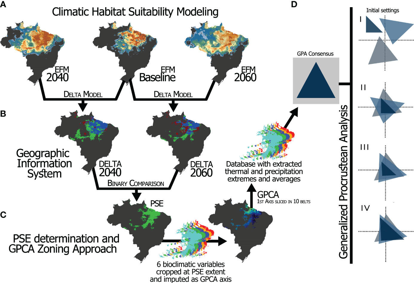
Figure 2 Main steps showing environmental layer extraction, how datasets from different period are overlapped and how Procrustes superimposition analysis is conducted. (A) Environmental modeling (above) resulting in habitat/climate suitability. (B) Extraction of datasets containing all variables obtained from modeling in (A). (C) Determination of the spatial extent of the PSE zone and application of the GPCA approach using the values of the bioclimatic layers cropped in this respective area as axis. (D) Procrustes superimposition showing a triangle configuration as a model: (I) original configurations, (II) being translated to superimpose their centroids (III) rotating and reflecting their corresponding vertices (tips) to the same position, (IV) and scaling them to maximize their coincidence by minimizing the sum of the squared deviations.
We obtained 134 unique records of Melipona fasciculata to run species distribution models after the data filtering (Database available at Supplementary Material 1). Among the 19 variables initially considered, 13 were maintained after collinearity evaluation (see Sup. Mat. 2). Out of the 125 computed models, 33 showed high predictive quality (TSS>0.8) and were kept for the ensemble forecasting. Among the algorithms, Random Forest had the best performance, contributing 12 models, then GAM with 7, Maxent and GBM with 6 each, and GLM with only 2 models. (see Sup. Mat. 3 and 4). Some areas of uncertainty regarding suitability prediction were detected in South American countries. However, in the focal area of the study, comprising the administrative extension of Brazil, only a few islands with the lowest level of uncertainty were detected in the northeast (access Supplementary Material 6 for details).
The ensembles were projected on maps (Figure 3) showing the variation of climate suitability for the species according to the three scenarios: baseline and respective projections for both future periods 2021-2040 (referred as 2040) and 2041-2060 (referred as 2060).
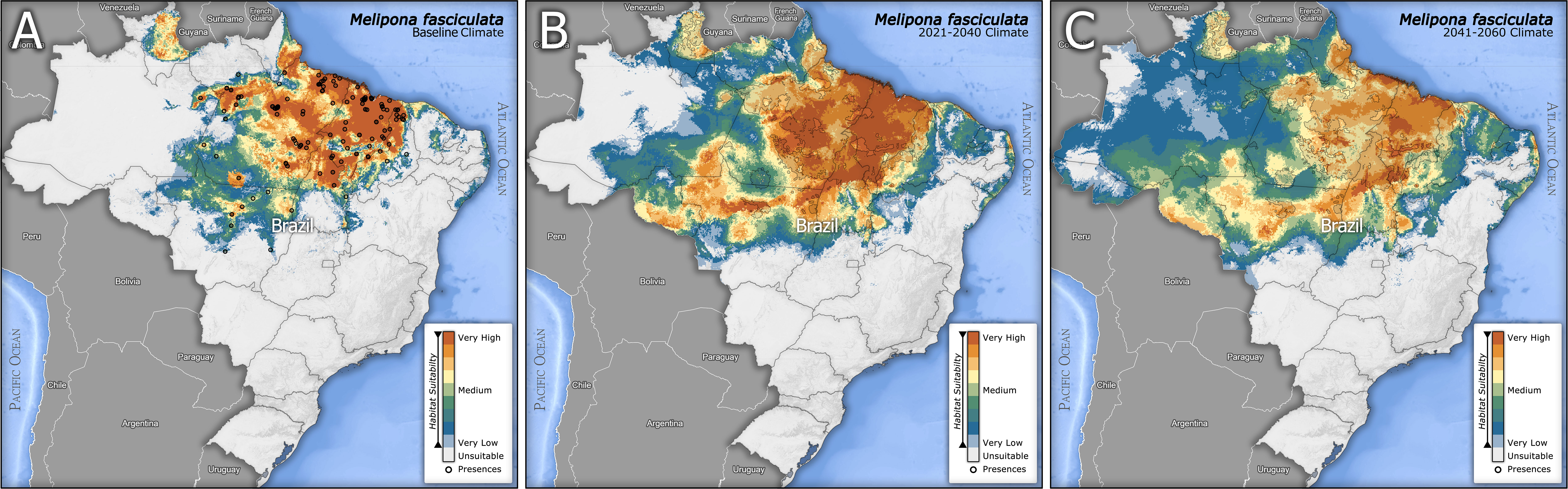
Figure 3 Ensemble models showing the climatic suitability at continuous values for Melipona fasciculata in Baseline (A), Future 2021-2040 (B) and Future 2041-2060 scenarios (C). The black dots in (A) represent the presence records of M. fasciculata. The hatched polygon over (B, C) (better visualized in the high-resolution figures) represent the extent of the baseline climatic suitability in a binary classification (Suitability >=0.75 to 1 reclassified to Bin=1), aiming at an easier comparison between baseline and future scenarios.
After the binary classification, the differences in suitability between baseline and future scenarios can be identified in the delta maps (Future minus Baseline EFM; Figure 4). We geospatially compared the delta maps and kept only the common areas that will remain (from baseline) suitable in all future periods. Thus, the blue areas of both maps (Figure 4) that overlap in space, as well as the gain zones in 2040 that remain suitable until 2060, were cropped, combined and mapped (Figure 5), composing the persistent suitable extent (PSE) displayed in Figure 5. The colored bands on this extent display the PCAZ, whose zones range in colors from dark blue (PCAZ zone 1) to yellow (PCAZ zone 10). Our PCAZ showed a pattern of undulating belts, cutting the PSE into ten irradiating zones from southeast to northwest. The map shows some smaller and spatially more restricted belts (PCAZ zone 9 and 10), and others quite extensive (PCAZ zone 4 and 3), and still others fragmented and with isolated islands (PCAZ zone 1 and 7). GPA applied to this layer enabled to calculate the intensities and trends of climate change from baseline to future per PCAZ.
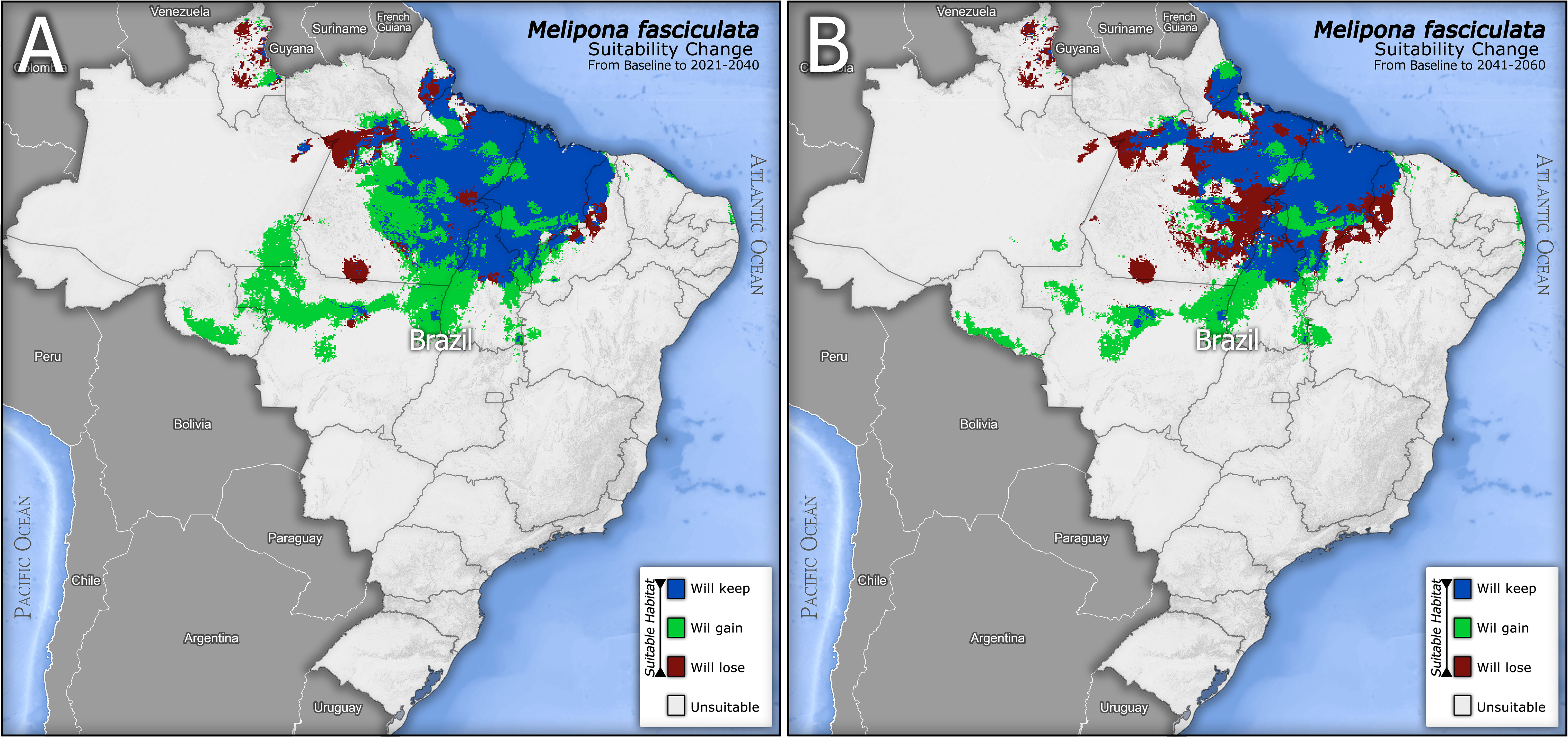
Figure 4 Differences between baseline and future climate suitability projections for Melipona fasciculata for the two future predictions: 2021-2040 (A) and 2041-2060 (B). The white and light tones represent the unsuitable areas for the species in Brazil; red represents previously suitable areas that will be lost; green represents climate suitable gained areas; and blue represents the areas that are currently climate suitable and will be kept in future scenarios.
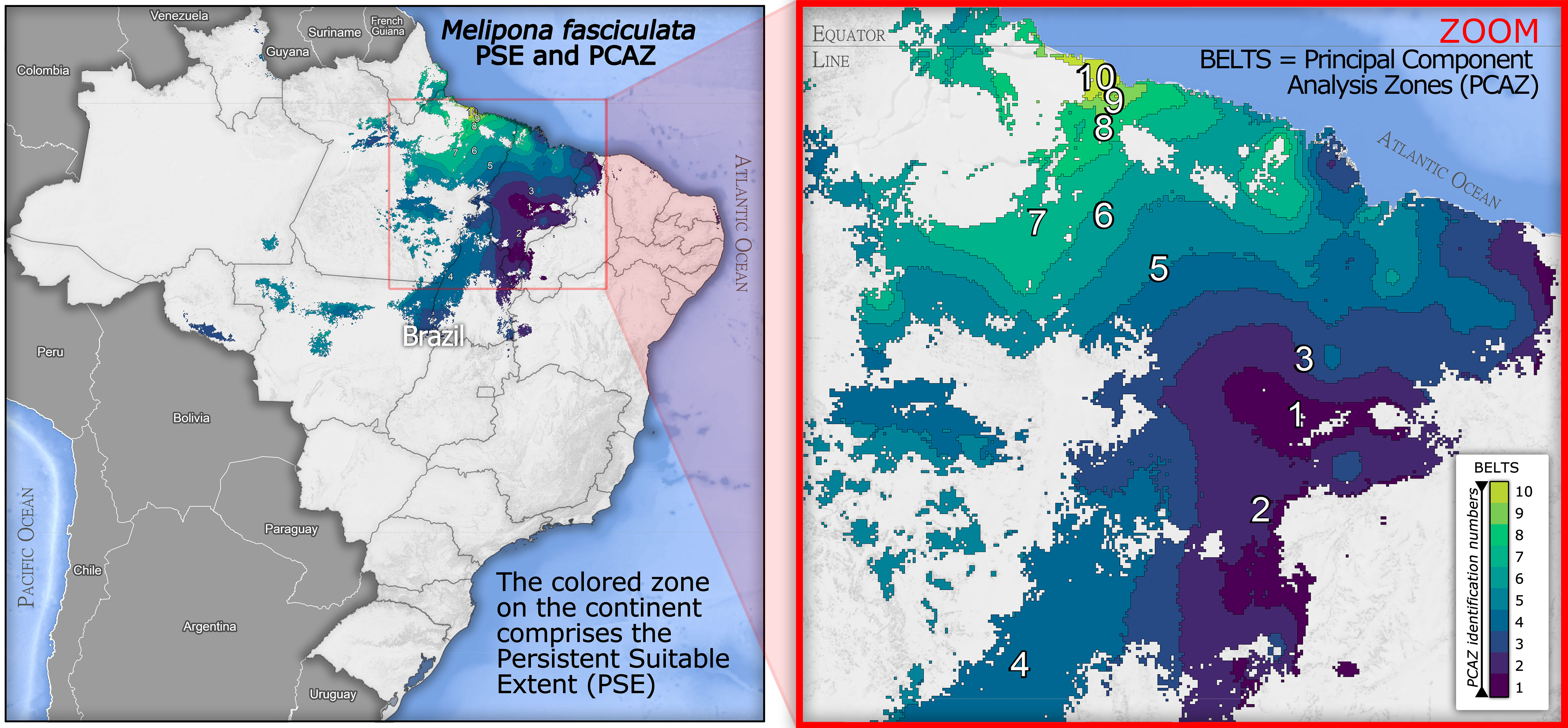
Figure 5 The total extent of the colored area in Brazil represents the Persistent Suitable Extent (PSE) for Melipona fasciculata considering all scenarios. The map also shows the ten PCAZ belts (ranging from green to blue) that spatially express the climatic variability over the area, whose variation was analyzed in detail through GPA.
We observed a significant projection of the bioclimatic variables through the multidimensional space of GPA (Permutation test; Rc = 99.79, p-value < 0.001; Figures 6A, B). The GPA model had an excellent fit (94.7%; Table 1), suggesting the occurrence of a common structure underlying how bioclimatic variables were projected among the different scenarios. Furthermore, the first two Procrustes dimensions accounted for 71.88% of the variation (dimension 1: 58.46%; dimension 2: 13.42%; respectively X and Y axis for Baseline, 2040 and 2060 frames in Figure 6C). This suggests that the positioning of these variables was different from the centroid and other individual configurations indicating that each bioclimatic variable could be properly distinguished according to its behavior in the multidimensional space. Our analysis reveals that nearly all bioclimatic variables were relevant with respect to the amount of explained variation for the consensus configuration (Table 1). Overall, our findings indicate that climatic similarity between both Baseline and 2040 scenarios will achieve 78% (Table 1 and 2040 frame in Figure 6B) within the next two decades, while the similarity between the baseline and 2060 scenarios is assumed to be more discordant from baseline with 64% (Table 1 and 2060 frame in Figure 6B).
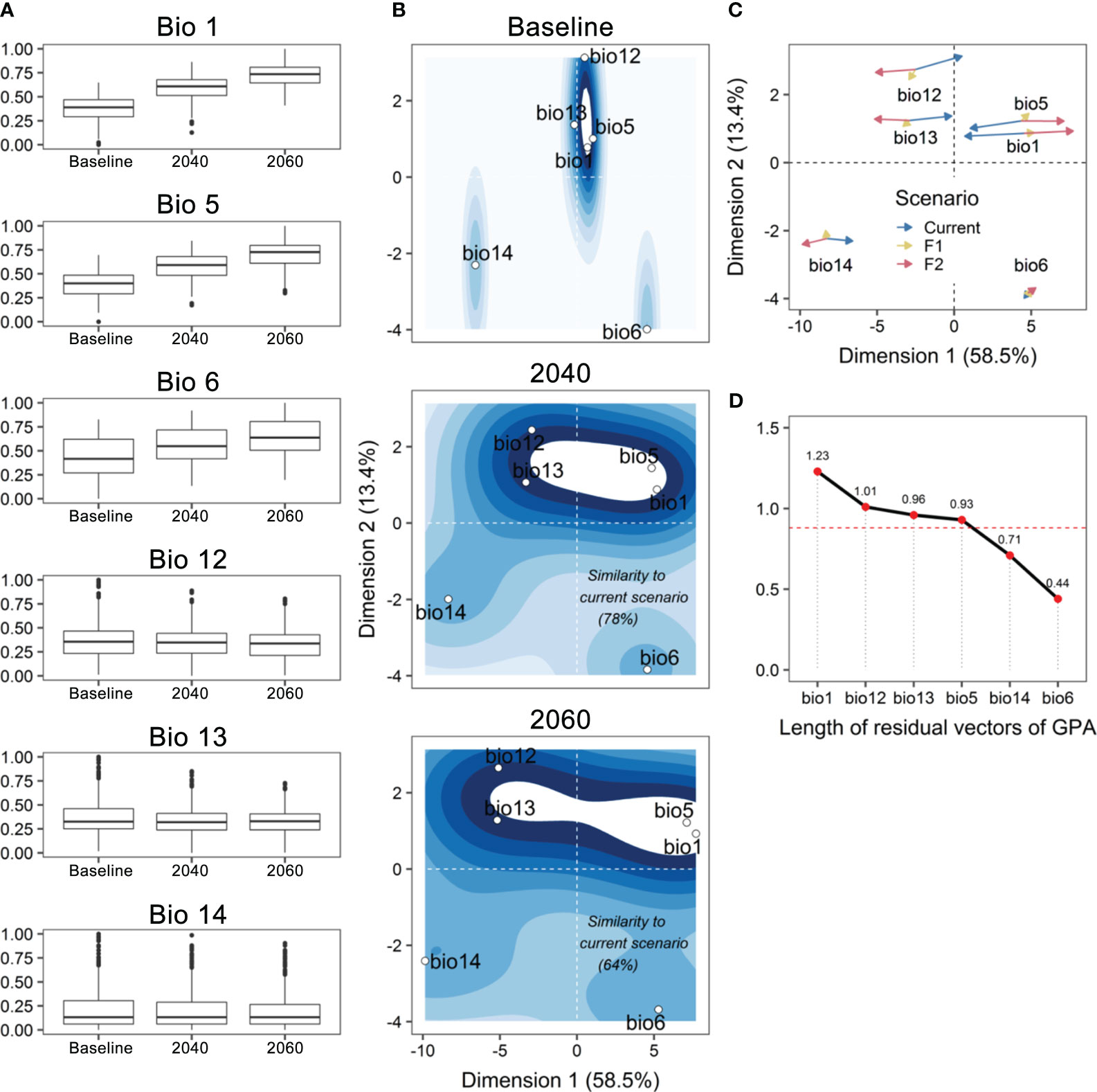
Figure 6 (A) Boxplots with the effects of the main six bioclimatic variables over the distribution area of Melipona fasciculata along the three scenarios. (B) Decomposition of residual sum of squares resulting from Generalized Procrustes Analysis representing the behavior (positioning, displacement) of each bioclimatic variable (white circles) in the multidimensional space. The contour lines were incorporated to this plot to facilitate the visualization of both the displacement and the discordance between scenarios (F1 = 2021-2040; F2 = 2041-2060). The percentage of similarity of both 2021-2040 and 2041-2060 periods to the baseline scenario was additionally included in the corresponding panels. (C) Generalized Procrustes Analysis map showing the trajectories (proximity, distance) and the length of residuals indicated by the arrows (i.e., amount of distortion from consensus configuration) of each bioclimatic variable throughout three climate scenarios. The higher the residuals, the larger discrepancies to match with the consensus configuration. (D) Therefore, greater residuals suggest higher within-variances in a particular variable and, thus, more difficulty to find an overall concordance between that variable along three assessed periods. Red dashed line is the average residual (0.88).
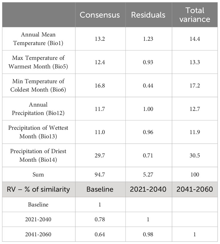
Table 1 Procrustes Analysis of Variance (PANOVA) summarizing the total variability in the bioclimatic variables and the pairwise similarity (in percentage) among periods according to combined variance of all six bioclimatic variables examined.
The main variables contributing to this climate disparity appear to be Bio1 (annual mean temperature) and Bio12 (annual precipitation), with the highest residual vector being observed in Bio1 (1.23; Figure 6D) followed by Bio12 (1.01; Figure 6D) among the six bioclimatic variables (Table 1). This means that it has a greater effect size, i.e., an elevated intra-variance resulting in a low concordance among three evaluated scenarios. Thus, it somehow suggests that Bio1 will likely have a more pervasive shift over the distribution area of M. fasciculata in the next decades. The Bio12 closely followed Bio1 in terms of the observed residual variance, having the second most discrepant residual vector (1.01). These results demonstrate that both variables are expected to behave with more uncertainty toward the next decades. Consequently, a rise in annual mean temperatures together with a decrease in annual precipitation might affect more drastically the distribution of M. fasciculata in the coming decades.
As we plot the scaled values of bioclimatic zones, we can overall observe a similar pattern in its within-variance. However, the PCAZ 9 and 10 seem to behave slightly different (Figures 7A, B; Table 2), being GPA robust enough to corroborate this. As such, there was a significant effect of the PCAZ along multidimensional space of GPA (Permutation test; Rc = 99.93, p-value < 0.001), with a near perfect fitting of the GPA model (99.9%). This indicates a shared zoning structure being projected along the different scenarios. Nevertheless, the first two Procrustes dimensions accounted for only 30.15% of the observed variation (dimension 1: 17.2%; dimension 2: 12.9%; Table 2, Figure 7B). This low explanatory value represented by the position of the climatic zones (located next to the center of configuration) reveals that adjacent zones were more like each other than expected (Figure 7A). As such, its behavior along the multidimensional space becomes harder to discriminate. However, at least three geographical regions emerge as good candidates for future ecological and molecular investigations, namely the geographical regions covered by PCAZ 9 and 10, in order to contrast their populations with each other, as well as from them to the populations in the remaining aggregated PCAZs, especially by comparing PCAZ 9 and 10 with those located in the more distant PCAZ, 1 to 4 (Table 2, Figure 7A). These three regions were positioned far from each other (Figure 7B) with higher positive values in the first two dimensions analyzed. Furthermore, they presented larger residues that can be observed by their values in Table 1 and the size of the arrows (Figures 7B, C). Although the small overall climate variability between the 10 PCAZ, especially when comparing adjacent PCAZ (Figure 7D), the process of discriminating the variable climate effects in the persistent suitability area (PSE) was efficient in supporting long-term sampling prioritizations.
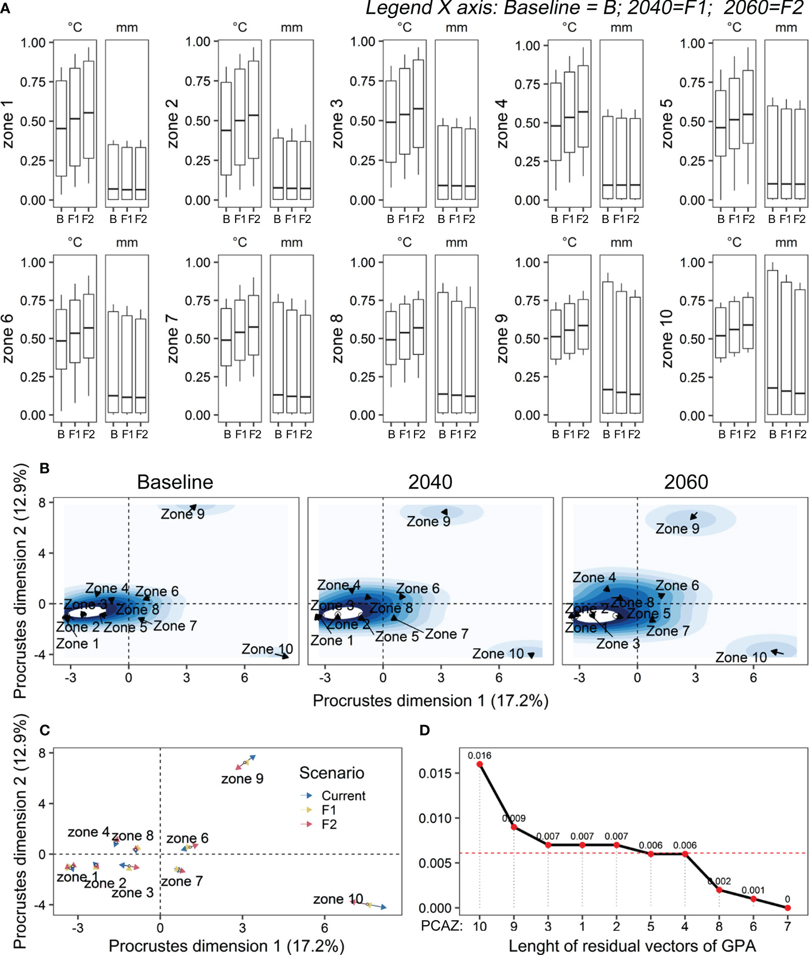
Figure 7 (A) Variation of temperature (°C) and precipitation (mm) along three periods (C = baseline; F1 = 2021-2040; F2 = 2041-2060) over 10 zones (PCAZ) extracted from GPCA in the distribution area of Melipona fasciculata. (B) Decomposition of residual sum of squares resulting from Generalized Procrustes Analysis representing the behavior (positioning, displacement) of each zone (black arrows) in the multidimensional space. The contour lines were incorporated to this plot to facilitate the visualization of displacement and how discordant were each scenario from each other. (C) Generalized Procrustes Analysis map showing the trajectories (proximity, distance) and length of residuals indicated by the arrows (i.e., amount of distortion from consensus configuration) of each zone throughout the three climate scenarios. The higher the residuals, the larger discrepancies to the consensus configuration. (D) Therefore, greater residuals suggest higher within-variances in a particular zone and, thus, more difficulty to find an overall concordance between that zone along three assessed periods. Red dashed line is the average residual (0.0061).
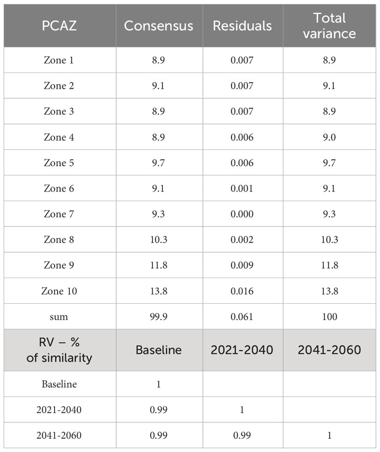
Table 2 Procrustes Analysis of Variance (PANOVA) summarizing the total variability in the PCAZ after Generalized Procrustes Analysis transformations per configuration and the pairwise similarity (in percentage) among periods according to combined variance of all ten bioclimatic zones evaluated (zones according Figure 5).
Our spatially explicitly results indicate important changes in habitat suitability for the species Melipona fasciculata, highlighting zones of gain, persistence, and loss of suitability. These findings provide support to the determination of conservation planning and population management actions to safeguard genetic variability of this species in the face of climate change. The areas of loss can guide monitoring actions and potential population translocation strategies from regions severely impacted by climate change. The areas of suitability persistence will be essential for the conservation of local populations and, depending on prior ecological assessments, may receive managed populations from areas of loss. Conversely, for the areas of suitability gain, it cannot be assured that they will effectively act as climatic refuges, as the timeframe of the results may be too short for a natural dispersal process on a broad geographical scale. However, they may also be of interest for assisted management, but this requires a very cautious prior assessment to avoid impacts on the species that already inhabit the sites, particularly other bees in terms of negative interactions, which could induce competition for resources with the risk of species exclusion and/or spread/spillover of diseases between specimens and species.
Previous studies already focused in the impact of climate change on the distribution of Brazilian stingless bees (Meliponini) (e.g., Giannini et al., 2012), showing detrimental losses of suitable habitat in the future. Other works highlighted the relationships with plants used by the bees (Giannini et al., 2013), and crop production (Giannini et al., 2017). Studies conducted in a preserved area of the eastern Amazon, in the Carajás National Forest, however, highlighted the extent of the problem, examining the impact of climate change on 216 bee species collected in the area: 85% of them would not find survival conditions in this forest by 2050-2070. Other work presented data on the climatic impacts on Melipona bee species used in Brazilian meliponiculture (Lima and Marchioro, 2021). This work highlights the future distribution areas for each species, with gains and losses depending on the species considered. In Colombia, ten Meliponini species were analyzed, considering the genera Melipona, Paratrigona, Plebeia, Frieseomelitta, and Scaura (Gonzalez et al., 2021). For most of them, the evidence indicated habitat loss in the coming years, with habitat gains for only two species. Also in the dry areas of Brazil, other analyses estimated the impact of climate change for Plebeia flavocincta (Maia et al., 2020), a small stingless bees largely used for meliponiculture.
By using our methodological framework, we were able to reveal that changes of climate variability are concordant throughout three scenarios. In short, while the three temperature variables tend to increase, the three precipitation variables seem to decrease. By integrating these results with the Procrustes analysis, it is possible to observe an expansion in the potential distribution area considering the future scenarios. This tendency was likely due to the position of all variables that progressively (from baseline to 2040 and 2060) move away from consensus configuration over the multidimensional space of Procrustes. These displacements of variables probably cause the observed disparity between 2040 and 2060 scenarios to the baseline climate. As a result, it should be expected a significant climate inconsistency within the geographic range of M. fasciculata in the next two decades baseline with an expected climate incompatibility of up to 22%. In fact, such mismatching might be still higher, achieving 36% of incompatibility within the next four decades.
The size of residuals was calculated by evaluating the difference between the location of the items of each configuration and the position of the item in the consensus configuration being, therefore, a good predictor of within-group variance (Gower, 1975; Ten Berge, 1977; Dijksterhuis and Gower, 1991; Goodall, 1991; Risvik et al., 1994). Here, the variance of each environmental variable provides a measure of deviation from the average scenario or GPCA Zones (referred as PCAZ). Consequently, it is possible to select the main zones according to the size of their residuals, which means that they likely have a larger effect on the different climatic scenarios.
The 10 zones partitioned within the persistent suitability area for M. fasciculata among the three scenarios presented varying levels of deviations from the consensus configuration, with PCAZ 9 and 10 standing out as better candidates for further surveying and/or monitoring. Both zones are located further northwest of the suitable habitat for M. fasciculata. Nevertheless, despite being adjacent to each other, zone 10 had the highest variance, with nearly twice the variance observed in zone 9. The comparison of these two PCAZ with the others, especially with the more distant ones (1-4), also proves to be an important prioritization to evaluate the differential climate effect between populations in the long term. Even though these three geographic regions (covering 9, 10 and 1-4 PCAZ) are within the appropriate climatic limits for the species until 2060, climate change will clearly generate effects of different intensities on their populations, which will possibly respond differently.
The final maps provided by our framework are ease to interpret, which allows estimating which changes might be expected with respect to the geographic range of target organisms over time assuming different climate change scenarios. Nevertheless, a more robust comparison among scenarios may be restrained by the lack of available data. Here we show that the Procrustes analysis was successful in accurately describing and quantifying the concordance among the evaluated scenarios and zones.
The use of more recent climate suitability models integrated with the Procrustes analysis was able to map and accurately describe the level of change among scenarios on the geographic distribution area of the studied species, highlighting distortions among bioclimatic variables of interest and pointing out areas of interest for decision-makers. Our framework also identified the environmental variables with higher relative importance among scenarios according to the size of their residuals. Accordingly, some zones along the distribution area of the target species can be prioritized for permanent monitoring of impacts on the species due to the expected higher change. Furthermore, some other zones, in which the climate change will be likely less pronounced, can be selected to act as a potential climate refuge. These areas could be prioritized to their conservation to sustain sanctuaries where the target species might continue to thrive.
Global conventions and reports continually issue warnings to assess and conserve biodiversity in the face of climate change. However, for such demands to be effectively met, the scientific community needs to develop operationalization strategies and orientation in more intuitive and simplified results to effectively convey the message to a wider audience. Research whose outcomes are presented in a complex way, requiring extensive scientific experience to be understood and interpreted, make it difficult to access fundamental information for decision-making at crucial moments, when scientific knowledge must be guided to support immediate action.
Analysis that generates spatially explicit results, especially presented through maps, have been an efficient support to decision making. With such support, they can point out where, when, and how they should act aiming reliable conservation and restoration plans. Besides these maps, the measure that quantifies percentages of change among baseline and future scenarios and the level of variance (degree of deviation) among variables of interest, may reinforce the evidence being sustained along studies of species distribution modeling and climate change modeling.
The combined use of Species Distribution Modeling (SDM) and Generalized Procrustes Analysis (GPA) provided a comprehensive approach for pollinator biomonitoring programs, such as bees, in the face of contemporary environmental challenges like climate change and biodiversity loss. SDM is essential for assessing the current and future climatic suitability of species, identifying critical areas that require conservation and restoration interventions. Combining SDM with GIS (Geographic Information System) offers clear visual representations of species distribution changes under different climate scenarios. In contrast, GPA allows for the assessment of concordance between climate scenarios and the identification of zones with significant variations. The integration of these analytical approaches deepens our understanding of climate change impacts on pollinators, prioritizes areas for conservation, sustainable use and research, and facilitates scientific communication, making information accessible for conservation decisions and nature-based solutions. We also suggest the need to identify areas for continuous monitoring of bee populations, following the considerations of Hoban et al. (2023) for biodiversity in general, and our proposed methodology fits this goal.
The original contributions presented in the study are included in the article/Supplementary Material, further inquiries can be directed to the corresponding author.
The manuscript presents research on animals that do not require ethical approval for their study.
AA: Conceptualization, Data curation, Formal analysis, Investigation, Methodology, Writing – original draft, Writing – review & editing, Resources, Visualization. CdS: Data curation, Formal Analysis, Methodology, Writing – original draft, Writing – review & editing. VI-F: Conceptualization, Funding acquisition, Resources, Supervision, Writing – original draft, Writing – review & editing. RO: Methodology, Visualization, Writing – review & editing, Writing – original draft. TG: Conceptualization, Funding acquisition, Supervision, Writing – original draft, Writing – review & editing.
The author(s) declare financial support was received for the research, authorship, and/or publication of this article. Instituto Tecnológico Vale (CNPq/ITV 4443.384/2018-9 and ITV R100603.83). Nacional Council of Scientific and Technological Development (CNPq) supported this research (444-384/2018-9).
CS thanks the CNPq 309542/2020-0, VLIF thanks CNPq 312250/2018-5. We also thank Rafael Cabral Borges and Marcela de Matos Barbosa for sharing data on Melipona fasciculata occurrences and collecting bee samples for further studies.
The authors declare that the research was conducted in the absence of any commercial or financial relationships that could be construed as a potential conflict of interest.
All claims expressed in this article are solely those of the authors and do not necessarily represent those of their affiliated organizations, or those of the publisher, the editors and the reviewers. Any product that may be evaluated in this article, or claim that may be made by its manufacturer, is not guaranteed or endorsed by the publisher.
The Supplementary Material for this article can be found online at: https://www.frontiersin.org/articles/10.3389/frbee.2024.1329844/full#supplementary-material
Acosta A. L., Giannini T. C., Imperatriz-Fonseca V. L., Saraiva A. M. (2016). Worldwide alien invasion: a methodological approach to forecast the potential spread of a highly invasive pollinator. PloS One 11 (1), e0148295. doi: 10.1371/journal.pone.0148295
Aguirre-Gutiérrez J., Carvalheiro L. G., Polce C., van Loon E. E., Raes N., Reemer M., et al. (2013). Fit-for-purpose: Species distribution model performance depends on evaluation criteria – dutch hoverflies as a case study. PloS One 8 (5), e63708. doi: 10.1371/journal.pone.0063708
Allouche O., Tsoar A., Kadmon R. (2006). Assessing the accuracy of species distribution models: prevalence, kappa and the true skill statistic (TSS). J. Appl. Ecol. 43 (6), 1223–1232. doi: 10.1111/j.1365-2664.2006.01214.x
Almeida A. G. S. (2022). Fidelidade Floral, Plasticidade Comportamental e Forrageamento Individual da Abelha Sem Ferrão Melipona (Melikerria) fasciculata Smith 1854, 197. Tese(Programa de Pós-graduação em Biotecnologia - Renorbio/CCBS)- Universidade Federal do Maranhão,. São Luís, Brazil.
Angelieri C. C. S., Adams-Hosking C., Paschoaletto K. M., de Barros Ferraz M., de Souza M. P., McAlpine C. A. (2016). Using species distribution models to predict potential landscape restoration effects on puma conservation. PloS One 11, 1–18. doi: 10.1371/journal.pone.0145232
Barbosa M. M., Jaffé R., Carvalho C. S., Lanes É.C.M., Alves-Pereira A. (2022). Landscape influences genetic diversity but does not limit gene flow in a Neotropical pollinator. Apidologie 53 (4), 483–493. doi: 10.1007/s13592-022-00916-9
Bramardi S. J., Bernet G. P., Asíns M. J., Carbonell E. A. (2005). Simultaneous agronomic and molecular characterization of genotypes via the Generalized Procrustes Analysis: An application to cucumber. Crop Sci. 45 (4), 1603–1609. doi: 10.2135/cropsci2004.0633
Breiman L. (2001). In Machine Learning Vol. 45 (Berlim/Heidelberg, Germany: Springer Science and Business Media LLC), 5–32. doi: 10.1023/a:1010933404324
Camiz S., Torres P., Pillar V. D. (2017). Recoding and multidimensional analyses of vegetation data: A comparison. Community Ecol. 18 (3), 260–279. doi: 10.1556/168.2017.18.3.5
Chaplin-Kramer R., Dombeck E., Gerber J., Knuth K. A., Mueller N. D., Mueller M., et al. (2014). Global malnutrition overlaps with pollinator-dependent micronutrient production. In Proc. R. Soc. B: Biol. Sci. 281 (1794), 20141799. doi: 10.1098/rspb.2014.1799
Chefaoui R. M., Lobo J. M. (2008). Assessing the effects of pseudo-absences on predictive distribution model performance. Ecol. Model. 210, 478–486. doi: 10.1016/j.ecolmodel.2007.08.010
Cheng S., Zeng W., Wang J., Liu L., Liang H., Kou Y., et al. (2021). Species delimitation of asteropyrum (Ranunculaceae) based on morphological, molecular, and ecological variation. Front. Plant Sci. 12. doi: 10.3389/fpls.2021.681864
Cortopassi-Laurino M., Imperatriz-Fonseca V. L., Roubik D. W., Dollin A., Heard T., Aguilar I., et al. (2006). Global meliponiculture: Challenges and opportunities. Apidologie 37, 275–292. doi: 10.1051/apido:2006027
Dijksterhuis G. B., Gower J. C. (1991). The interpretation of Generalized Procrustes Analysis and allied methods. Food Qual. Preference 3, 67–87. doi: 10.1016/0950-3293(91)90027-C
Diniz-Filho J. A. F., Mauricio Bini L., Fernando Rangel T., Loyola R. D., Hof C., Nogués-Bravo D., et al. (2009). Partitioning and mapping uncertainties in ensembles of forecasts of species turnover under climate change. Ecography 32, 897–906. doi: 10.1111/j.1600-0587.2009.06196.x
dos Santos C. F., Souza dos Santos P. D., Marques D. M., Da-Costa T., Blochtein B. (2019). Geometric morphometrics of the forewing shape and size discriminate Plebeia species (Hymenoptera: Apidae) nesting in different substrates. Systematic Entomology 44, 787–796. doi: 10.1111/syen.12354
Engel M. S., Rasmussen C., Ayala R., de Oliveira F. F. (2023). Stingless bee classification and biology (Hymenoptera, Apidae): a review, with an updated key to genera and subgenera. Zookeys 1172, 239–312. doi: 10.3897/zookeys.1172.104944
Espíndola A., Pliscoff P. (2018). The relationship between pollinator visits and climatic suitabilities in specialized pollination interactions. Ann. Entomological Soc. America 112 (3), 150–157. doi: 10.1093/aesa/say042
Farfan S. J. A., Celentano D., Silva Junior C. H.L., de Freitas Silveira M. V., Serra R. T.A., Gutierrez J. A.M., et al. (2022). The effect of landscape composition on stingless bee (Melipona fasciculata) honey productivity in a wetland ecosystem of Eastern Amazon, Brazil. J. Apic. Res. 62 (5), 1102–1114. doi: 10.1080/00218839.2022.2137307
Ferraz K., Ferraz S., Paula R. C., Beisiegel B., Breitenmoser C. (2012). Species distribution modeling for conservation purposes. Natureza Conservação 10, 214–220. doi: 10.4322/natcon.2012.032
Fick S. E., Hijmans R. J. (2017). WorldClim 2: New 1-km spatial resolution climate surfaces for global land areas. Int. J. Climatology 37 (12), 4302–4315. doi: 10.1002/joc.5086
Foden W. B., Young B. E., Akçakaya H. R., Garcia R. A., Hoffmann A. A., Stein B. A., et al. (2018). Climate change vulnerability assessment of species. WIREs Climate Change 10 (1), e551. doi: 10.1002/wcc.551
Gavioli A., de Souza E. G., Bazzi C. L., Guedes L. P. C., Schenatto K. (2016). Optimization of management zone delineation by using spatial principal components. Comput. Electron. Agric. 127, 302–310. doi: 10.1016/j.compag.2016.06.029
GBIF (2023). Occurrence Download [Melipona fasciculata Smith, 1854]. The global biodiversity information facility. GBIF.org. doi: 10.15468/DL.GVXE6Y
Giannini T. C., Acosta A. L., da Silva C. I., de Oliveira P. E. A. M., Imperatriz-Fonseca V. L., Saraiva A. M. (2013). Identifying the areas to preserve passion fruit pollination service in Brazilian Tropical Savannas under climate change. Agriculture Ecosyst. Environ. 171, 39–46. doi: 10.1016/j.agee.2013.03.003
Giannini T. C., Acosta A. L., Garófalo C. A., Saraiva A. M., Alves-dos-Santos I., Imperatriz-Fonseca V. L. (2012). Pollination services at risk: Bee habitats will decrease owing to climate change in Brazil. Ecol. Model. 244, 127–131. doi: 10.1016/j.ecolmodel.2012.06.035
Giannini T. C., Boff S., Cordeiro G. D., Cartolano E. A., Veiga A. K., Imperatriz-Fonseca V. L., et al. (2015). Crop pollinators in Brazil: a review of reported interactions. Apidologie 46, 209–223. doi: 10.1007/s13592-014-0316-z
Giannini T. C., Costa W. F., Cordeiro G. D., Imperatriz-Fonseca V. L., Saraiva A. M., Biesmeijer J., et al. (2017). Projected climate change threatens pollinators and crop production in Brazil. PloS One 12 (8), e0182274. doi: 10.1371/journal.pone.0182274
Gonzalez V. H., Cobos M. E., Jaramillo J., Ospina R. (2021). Climate change will reduce the potential distribution ranges of Colombia’s most valuable pollinators. Perspect. Ecol. Conserv. 19 (2), 195–206. doi: 10.1016/j.pecon.2021.02.010
Goodall C. (1991). Procrustes methods in the statistical analysis of shape. J. R. Stat. Society: Ser. B (Methodological) 53, 285–321. doi: 10.1111/j.2517-6161.1991.tb01825.x
Gostinski L. F., Oliveira F. F., Contrera F. A. L., Albuquerque P. M. C. (2018). Trophic niche and floral resources partition between two species of Melipona (Hymenoptera, Apidae) in the Eastern Amazon. Oecologia Australis 22, 449–462. doi: 10.4257/oeco.2018.2204.08
Gower J. C. (1975). Generalized procrustes analysis. Psychometrika 40, 33–51. doi: 10.1007/BF02291478
Greenwell B., Boehmke B., Cunningham J., GBM-Developers (2020) gbm Generalized Boosted Regression Models. Available at: https://cran.rproject:web/packages/gbm/index.html.
Guisan A., Thuiller W. (2005). Predicting species distribution: offering more than simple habitat models. Ecol. Lett. 8, 993–1009. doi: 10.1111/j.1461-0248.2005.00792.x
Guisan A., Tingley R., Baumgartner J. B., Naujokaitis-Lewis I., Sutcliffe P. R., Tulloch A. I. T., et al. (2013). Predicting species distributions for conservation decisions. Ecol. Lett. 16, 1424–1435. doi: 10.1111/ele.12189
Hao T., Elith J., Guillera-Arroita G., Lahoz-Monfort J. J. (2019). A review of evidence about use and performance of species distribution modeling ensembles like BIOMOD. Diversity Distributions 25, 839–852. doi: 10.1111/ddi.12892
Hastie T. J., Pregibon D. (1992). “Generalized linear models,” in Statistical Models S (Chapter 6). Eds. Chambers M., Hastie T. J. (Pacific Grove, CA, U.S.A.: Wadsworth & Brooks/Cole).
Hastie T. J., Tibshirani R. J. (1990). Generalized additive models. Chapman & Hall/CRC Monographs on Statistics & Applied Probability, Vol. 43. (Boca Raton, FL, U.S.A.: CRC Press).
Hausfather Z. (2019) CMIP6: the next generation of climate models explained. Available at: www.carbonbrief:cmip6-the-next-generation-of-climate-models-explained (Accessed January 2023).
Hegland S. J., Nielsen A., Lázaro A., Bjerknes A. L., Totland Ø., Vindenes Y. (2021). Climate-driven range shifts of bumblebee species and their extinction risk. Global Change Biol. 27 (1), 119–130. doi: 10.1111/gcb.15428
Hervé M. (2020) RVA de Memoire: Diverse basic statistical and graphical functions. Available at: http://cran.r-project.org/package=RVAideMemoire.
Hill R., Nates-Parra G., Quezada-Euán J. J. G., Buchori D., LeBuhn G., Maués M. M., et al. (2019). Biocultural approaches to pollinator conservation. Nat. Sustainability 2 (3), 214–222. doi: 10.1038/s41893-019-0244-z
Hirzel A. H., Le Lay G. (2008). Habitat suitability modeling and niche theory. J. Appl. Ecol. 45, 1372–1381. doi: 10.1111/j.1365-2664.2008.01524.x
Hoban S., da Silva J. M., Mastretta-Yanes A., Grueber C. E., Heuertz M., Hunter M. E., et al. (2023). Monitoring status and trends in genetic diversity for the Convention on Biological Diversity: An ongoing assessment of genetic indicators in nine countries. Conserv. Lett. 16 (3), e12953. doi: 10.1111/conl.12953
Hristov P., Neov B., Shumkova R., Palova N. (2020). Significance of apoidea as main pollinators. Ecological and economic impact and implications for human nutrition. Diversity 12 (7), 280. doi: 10.3390/d12070280
Huang M.-J., Hughes A. C., Xu C.-Y., Miao B.-G., Gao J., Peng Y.-Q. (2022). Mapping the changing distribution of two important pollinating giant honeybees across 21000 years. Global Ecol. Conserv. 39, e02282. doi: 10.1016/j.gecco.2022.e02282
Hulme P. E. (2005). Adapting to climate change: Is there scope for ecological management in the face of a global threat? J. Appl. Ecol. 42, 784–794. doi: 10.1111/j.1365-2664.2005.01082.x
IBGE. (2022). Malha Municipal Digital (MMD) da Divisão Político-Administrativa Brasileira – 2022. Available at: http://www.ibge.gov.br/geociencias/cartas_base/malhas_municipais/municipio_2022/.
IPCC-AR6 (2021). “Summary for Policymakers.” in Climate Change 2021 – The Physical Science Basis. V. Masson-Delmotte, Zhai P., Pirani A., S. L., et al. Eds. 3–32. doi: 10.1017/9781009157896.001
Jaffé R., Pope N., Carvalho A. T., Maia U. M., Blochtein B., Carvalho C. A. L., et al. (2015). Bees for development: Brazilian survey reveals how to optimize stingless beekeeping. PloS One 10, e0121157. doi: 10.1371/journal.pone.0121157
Jollife I. T., Cadima J. (2016). Principal component analysis: A review and recent developments. Philos. Trans. R. Soc. A: Mathematical Phys. Eng. Sci. 374 (2065), 20150202. doi: 10.1098/rsta.2015.0202
Kearney M. R., Wintle B. A., Porter W. P. (2010). Correlative and mechanistic models of species distribution provide congruent forecasts under climate change. Conserv. Lett. 3, 203–213. doi: 10.1111/j.1755-263X.2010.00097.x
Kerr J. T., Pindar A., Galpern P., Packer L., Potts S. G., Roberts S. M., et al. (2015). Climate change–mediated impacts on phenology and consequences for bumblebee fecundity. Proc. R. Soc. B 282 (1814), 2015–2023. doi: 10.1098/rspb.2015.0826
Klein A. M., Freitas B. M., Bonfim I. G. A., Boreaux V., Foroff F., Oliveira M. O. (2020). Insect Pollination of Crops in Brazil, a Guide For Farmers, Gardeners, Politicians And Conservationists. (Freiburg: Albert-Ludwigs University). 162p. doi: 10.6094/UNIFR/151200
Klein A.-M., Vaissière B. E., Cane J. H., Steffan-Dewenter I., Cunningham S. A., Kremen C., et al. (2007). Importance of pollinators in changing landscapes for world crops. Proc. R. Soc. B: Biol. Sci. 274, 303–313. doi: 10.1098/rspb.2006.3721
Klingenberg C. P. (2016). Size, shape, and form: concepts of allometry in geometric morphometrics. Dev. Genes Evol. 226, 113–137. doi: 10.1007/s00427-016-0539-2
Lê S., Josse J., Husson F. (2008). FactoMineR: An R package for multivariate analysis. J. Stat. Software 25, 1–18. doi: 10.18637/jss.v025.i01
Leutner B. (2022) RStoolbox: A Collection of Remote Sensing Tools. Available at: https://bleutner.github.io/RStoolbox/rstbx-docu/RStoolbox.html.
Li D., Wu S., Liu L., Zhang Y., Li S. (2018). Vulnerability of the global terrestrial ecosystems to climate change. Global Change Biol. 24, 4095–4106. doi: 10.1111/gcb.14327
Lima V. P., Marchioro C. A. (2021). Brazilian stingless bees are threatened by habitat conversion and climate change. Regional Environ. Change 21 (1), 14. doi: 10.1007/s10113-021-01751-9
Lisboa F. J. G., Peres-Neto P. R., Chaer G. M., Da Conceição Jesus E., Mitchell R. J., Chapman S. J., et al. (2014). Much beyond Mantel: Bringing procrustes association metric to the plant and soil ecologist’s toolbox. PloS One 9, e101238. doi: 10.1371/journal.pone.0101238
Ludena C. E., Yoon S. W. (2015). Local vulnerability indicators and adaptation to climate change: A survey (Washington, DC: Inter-American Development Bank), 51. (Technical Note No. 857).
Maia U. M., Miranda L., de S., Carvalho A. T., Imperatriz-Fonseca V. L., de Oliveira G. C., et al. (2020). Climate-induced distribution dynamics of Plebeia flavocincta, a stingless bee from Brazilian tropical dry forests. Ecol. Evol. 10 (18), 10130–10138. doi: 10.1002/ece3.6674
Marshall L., Leclercq N., Weekers T., El Abdouni I., Carvalheiro L. G., Kuhlmann M., et al. (2023). Potential for climate change driven spatial mismatches between apple crops and their wild bee pollinators at a continental scale. Global Environ. Change 83, 102742. doi: 10.1016/j.gloenvcha.2023.102742
Maués M. M., Couturier G. (2002). Biologia floral e fenologia reprodutiva do camu-camu (Myrciaria dubia (H.B.K.) McVaugh, Myrtaceae) no Estado Pará, Brasil. Rev. Bras. Botânica 25 (4), 441–448. doi: 10.1590/s0100-84042002012000008
Mauricio A. A., Palazzo A. B., Caselato V. M., Bolini H. M. A. (2016). Generalized Procrustes Analysis and external preference map used to consumer drivers of diet gluten free product. Food Nutr. Sci. 7, 711–723. doi: 10.4236/fns.2016.79072
Mcbride L. A., Hope A. P., Canty T. P., Bennett B. F., Tribett W. R., Salawitch R. J. (2021). Comparison of CMIP6 historical climate simulations and future projected warming to an empirical model of global climate. Earth System Dynamics 12, 545–579. doi: 10.5194/esd-12-545-2021
Mitteroecker P., Gunz P. (2009). Advances in geometric morphometrics. Evolutionary Biol. 36 (2), 235–247. doi: 10.1007/s11692-009-9055-x
Moure J. S., Urban D., Melo G. A. R. (2022) Catalogue of Bees (Hymenoptera, Apoidea) in the Neotropical Region – online version. Available at: http://moure.cria.org.br/catalogue.
Naimi B., Hamm N. A. S., Groen T. A., Skidmore A. K., Toxopeus A. G. (2014). Where is positional uncertainty a problem for species distribution modeling? Ecography 37, 191–203. doi: 10.1111/j.1600-0587.2013.00205.x
Nicola P. A., Monteiro L. R., Pessôa L. M., Von Zuben F. J., Rohlf F. J., dos Reis S. F. (2003). Congruence of hierarchical, localized variation in cranial shape and molecular phylogenetic structure in spiny rats, genus Trinomys (Rodentia: Echimyidae). Biol. J. Linn. Soc. 80, 385–396. doi: 10.1046/j.1095-8312.2003.00245.x
Nunes-Silva P., Costa L., Campbell A. J., Arruda H., Contrera F. A. L., Teixeira J. S. G., et al. (2020). Radiofrequency identification (RFID) reveals long-distance flight and homing abilities of the stingless bee Melipona fasciculata. Apidologie 51, 240–253. doi: 10.1007/s13592-019-00706-8
Nunes-Silva P., Hrncir M., Silva C. I., Roldão Y. S., Imperatriz-Fonseca V. L. (2013). Stingless bees, Melipona fasciculata, as efficient pollinators of eggplant (Solanum melongena) in greenhouses. Apidologie 44, 537–546. doi: 10.1007/s13592-013-0204-y
Ollerton J., Winfree R., Tarrant S. (2011). How many flowering plants are pollinated by animals? Oikos 120, 321–326. doi: 10.1111/j.1600-0706.2010.18644.x
Patel V., Pauli N., Biggs E., Barbour L., Boruff B. (2020). Why bees are critical for achieving sustainable development. Ambio 50, 49–59. doi: 10.1007/s13280-020-01333-9
Phillips S. J., Anderson R. P., Schapire R. E. (2006). Maximum entropy modeling of species geographic distributions. Ecol. Model. 190 (3–4), 231–259. doi: 10.1016/j.ecolmodel.2005.03.026
Phillips S. J., Dudík M., Schapire R. E. (2021). Maxent software for modeling species niches and distributions (Version 3.4.1). Available at: http://biodiversityinformatics.amnh.org/open_source/maxent/. (Accessed on July 7, 2021).
Potts S. G., Biesmeijer J. C., Kremen C., Neumann P., Schweiger O., Kunin W. E. (2010). Global pollinator declines: trends, impacts and drivers. Trends Ecol. Evol. 25, 345–353. doi: 10.1016/j.tree.2010.01.007
Potts S. G., Imperatriz-Fonseca V. L., Ngo H. T., Aizen M. A., Biesmeijer J. C., Breeze T. D., et al. (2016). Safeguarding pollinators and their values to human well-being. Nature 540, 220–229. doi: 10.1038/nature20588
Quezada-Euán J. J. G., Nates-Parra G., Maués M. M., Imperatriz-Fonseca V. L., Roubik D. W. (2018). Meliponini) among ethnic groups of tropical America. Sociobiology 65 (4), 534–557. doi: 10.13102/sociobiology.v65i4.3447
R Core Team (2021). R: A language and environment for statistical computing (Vienna, Austria: The R Foundation for Statistical Computing).
Ren G., Mateo R. G., Liu J., Suchan T., Alvarez N., Guisan A., et al. (2016). Genetic consequences of Quaternary climatic oscillations in the Himalayas: Primula tibetica as a case study based on restriction site-associated DNA sequencing. New Phytol. 213 (3), 1500–1512. doi: 10.1111/nph.14221
Risvik E., McEwan J. A., Colwill J. S., Rogers R., Lyon D. H. (1994). Projective mapping: A tool for sensory analysis and consumer research. Food Qual. Preference 5 (4), 263–269. doi: 10.1016/0950-3293(94)90051-5
Rodríguez-Noriega S., Buenrostro-Figueroa J. J., Rebolloso-Padilla O. N., Corona-Flores J., Camposeco-Montejo N., Flores-Naveda A., et al. (2021). Developing a descriptive sensory characterization of flour tortilla applying flash profile. Foods 10 (7), 1473. doi: 10.3390/foods10071473
Rohlf F. J. (1998). Geometric morphometrics and phylogeny. Systematic Biol. 47, 147–158. doi: 10.1080/106351598261094
Roubik D. W. (2023). Stingless bee (Apidae: Apinae: Meliponini) ecology. Annu. Rev. Entomology 68 (1), 231–256. doi: 10.1146/annurev-ento-120120-103938
Schonfeldt M., Klatt B. K., Schindler M., Westphal C. (2022). Climate-driven changes in the community composition of wild bees in Germany. Global Change Biol. 28 (4), 1216–1230. doi: 10.1111/gcb.15978
Schramek C. (2021) New Scenarios and Greater Certainty in IPCC AR6. Available at: https://greencentralbanking.com/2021/08/10/new-scenarios-and-greater-certainty-in-ipcc-ar6/.
Ser G. (2019). Using Generalized Procrustes Analysis for evaluation of sensory characteristic data of lamb meat. Turkish J. Agric. - Food Sci. Technol. 7, 840. doi: 10.24925/turjaf.v7i6.840-844.2214
Sgolastra F., Galloni M., Medrzycki P. (2022). Climate change impacts on wild bees: A review of recent research. Curr. Opin. Insect Sci. 55, 33–39. doi: 10.1016/j.cois.2022.02.004
Sofaer H. R., Jarnevich C. S., Pearse I. S., Smyth R. L., Auer S., Cook G. L., et al. (2019). Development and delivery of species distribution models to inform decision-making. Bioscience 69, 544–557. doi: 10.1093/biosci/biz045
Ten Berge J. M. F. (1977). Orthogonal procrustes rotation for two or more matrices. Psychometrika 42, 267–276. doi: 10.1007/BF02294053
Thuiller W., Georges D., Gueguen M., Engler R., Breiner F. (2021) biomod2: Ensemble platform for species distribution modeling. Available at: https://cran.r-project.org/package=biomod2.
Thuiller W., Lafourcade B., Engler R., Araújo M. B. (2009). BIOMOD – a platform for ensemble forecasting of species distributions. Ecography 32 (3), 369–373. doi: 10.1111/j.1600-0587.2008.05742.x
Venturieri G. C., Baquero P. L., Costa L. (2015). “Formação de Minicolônias de Uruçu-Cinzenta [Melipona fasciculata Smith 1858 (Apidae, Meliponini)],” in Belém, Pará: Empresa Brasileira de Pesquisa Agropecuária; Embrapa Clima Temperado; Ministério da Agricultura, Pecuária e Abastecimento Brasilia- Distrito Federal, Brasil.
Venturieri G. C., Leão K. L., Rêgo E., de S., Venturieri G. A. (2017). Honey production of the “uruçu-cinzenta” stingless bee (Melipona fasciculata) after offering cerumen in natural form or as artificially made pots. J. Apic. Res. 57 (1), 129–134. doi: 10.1080/00218839.2017.1339520
Viscosi V., Cardini A. (2011). Leaf morphology, taxonomy and geometric morphometrics: A simplified protocol for beginners. PloS One 6 (10), e25630. doi: 10.1371/journal.pone.0025630
Wakeling I. N., Raats M. M., MacFie H. J. H. (1992). A new significance test for consensus in Generalized Procrustes Analysis. J. Sensory Stud. 7, 91–96. doi: 10.1111/j.1745-459X.1992.tb00526.x
Wisz M. S., Hijmans R. J., Li J., Peterson A. T., Graham C. H., Guisan A. (2008). Effects of sample size on the performance of species distribution models. Diversity Distributions 14, 763–773. doi: 10.1111/j.1472-4642.2008.00482.x
Xiong R., Blot K., Meullenet J. F., Dessirier J. M. (2008b). Permutation tests for generalized procrustes analysis. Food Qual. Preference 19, 146–155. doi: 10.1016/j.foodqual.2007.03.003
Keywords: methodological framework, species distribution modeling, conservation, decision making, priority zones, climate change, stingless bee, Melipona fasciculata
Citation: Acosta AL, dos Santos CF, Imperatriz-Fonseca VL, Oliveira RC and Giannini TC (2024) A methodological approach to identify priority zones for monitoring and assessment of wild bee species under climate change. Front. Bee Sci. 2:1329844. doi: 10.3389/frbee.2024.1329844
Received: 30 October 2023; Accepted: 22 January 2024;
Published: 09 February 2024.
Edited by:
Christian W. W. Pirk, University of Pretoria, South AfricaReviewed by:
Jan Brus, Palacký University, Olomouc, CzechiaCopyright © 2024 Acosta, dos Santos, Imperatriz-Fonseca, Oliveira and Giannini. This is an open-access article distributed under the terms of the Creative Commons Attribution License (CC BY). The use, distribution or reproduction in other forums is permitted, provided the original author(s) and the copyright owner(s) are credited and that the original publication in this journal is cited, in accordance with accepted academic practice. No use, distribution or reproduction is permitted which does not comply with these terms.
*Correspondence: André Luis Acosta, YW5kcmVsdWlzYWNvc3RhQGdtYWlsLmNvbQ==
†ORCID: André Luis Acosta, orcid.org/0000-0002-4244-9637
Charles Fernando dos Santos, orcid.org/0000-0001-5181-2461
Vera Lucia Imperatriz-Fonseca, orcid.org/0000-0002-1079-2158
Ricardo Caliari Oliveira, orcid.org/0000-0002-8996-1291
Tereza Cristina Giannini, orcid.org/0000-0001-9830-1204
Disclaimer: All claims expressed in this article are solely those of the authors and do not necessarily represent those of their affiliated organizations, or those of the publisher, the editors and the reviewers. Any product that may be evaluated in this article or claim that may be made by its manufacturer is not guaranteed or endorsed by the publisher.
Research integrity at Frontiers
Learn more about the work of our research integrity team to safeguard the quality of each article we publish.