 Nathan Cornille
 Katrien Laenen
 Marie-Francine Moens
95% of researchers rate our articles as excellent or good
Learn more about the work of our research integrity team to safeguard the quality of each article we publish.
Find out more
ORIGINAL RESEARCH article
Front. Artif. Intell. , 17 March 2022
Sec. Machine Learning and Artificial Intelligence
Volume 5 - 2022 | https://doi.org/10.3389/frai.2022.736791
This article is part of the Research Topic Identifying, Analyzing, and Overcoming Challenges in Vision and Language Research View all 4 articles
An important problem with many current visio-linguistic models is that they often depend on spurious correlations. A typical example of a spurious correlation between two variables is one that is due to a third variable causing both (a “confounder”). Recent work has addressed this by adjusting for spurious correlations using a technique of deconfounding with automatically found confounders. We will refer to this technique as AutoDeconfounding. This article dives more deeply into AutoDeconfounding, and surfaces a number of issues of the original technique. First, we evaluate whether its implementation is actually equivalent to deconfounding. We provide an explicit explanation of the relation between AutoDeconfounding and the underlying causal model on which it implicitly operates, and show that additional assumptions are needed before the implementation of AutoDeconfounding can be equated to correct deconfounding. Inspired by this result, we perform ablation studies to verify to what extent the improvement on downstream visio-linguistic tasks reported by the works that implement AutoDeconfounding is due to AutoDeconfounding, and to what extent it is specifically due to the deconfounding aspect of AutoDeconfounding. We evaluate AutoDeconfounding in a way that isolates its effect, and no longer see the same improvement. We also show that tweaking AutoDeconfounding to be less related to deconfounding does not negatively affect performance on downstream visio-linguistic tasks. Furthermore, we create a human-labeled ground truth causality dataset for objects in a scene to empirically verify whether and how well confounders are found. We show that some models do indeed find more confounders than a random baseline, but also that finding more confounders is not correlated with performing better on downstream visio-linguistic tasks. Finally, we summarize the current limitations of AutoDeconfounding to solve the issue of spurious correlations and provide directions for the design of novel AutoDeconfounding methods that are aimed at overcoming these limitations.
Recent years have seen great progress in vision and language research. Increasingly complex models trained on very large datasets of paired images and text seem to capture a lot of the correlations that are needed to solve tasks such as Visual Question Answering or Image Retrieval.
A concern however is that models make many of their predictions based on so-called spurious correlations: correlations that are present in the training data, but do not generalize to accurately make predictions when confronted with real world data.
To address this concern, researchers increasingly study the integration of causation into models. A model that is able to solve problems in a causal way, will be faster to adapt to other distributions and thus be more generalizable (Schölkopf, 2019). Because there are often multiple possible underlying causal models that each perfectly match the observed statistics, a key challenge is that it is not always easy to discover causal structure in purely observational data without being able to perform interventions1 on the data.
Recently, a technique has been proposed that aims to automatically discover and use knowledge of the underlying causal structure in order to avoid learning spurious correlations. More specifically, the goal is to avoid learning correlations that are due to a common cause (or “confounder”)2, a process called “deconfounding.” We will further refer to this technique as AutoDeconfounding. AutoDeconfounding was first developed by Wang et al. (2020) in their model named VC-R-CNN, and more recently adapted to the multi-modal setting by Zhang et al. (2020b) in their model DeVLBERT.
The goal of this article is to critically examine the technique of AutoDeconfounding and theoretically and empirically investigate whether AutoDeconfounding is an effective method to avoid spurious correlations. A closer inspection of AutoDeconfounding raises a number of questions that are addressed in this article.
First, deconfounding implies a certain assumption on the type of causal variables and their possible values. We make the underlying causal model of AutoDeconfounding explicit, and use that model to show that additional assumptions are needed before the implementation of AutoDeconfounding can be equated to correct deconfounding.
Inspired by this observation, we then set out to investigate to what extent the reported improvement on downstream tasks is due to AutoDeconfounding, and to what extent it is specifically due to the deconfounding aspect of AutoDeconfounding. Focusing on the most recent article (Zhang et al., 2020b), that implements AutoDeconfounding in a visio-linguistic context, we retrain and evaluate their model (“DeVLBERT-repro”) and their baseline (“ViLBERT-repro”) in a way that isolates the contribution of AutoDeconfounding. We compare the scores for our reproductions with the reported scores, as well as with the score of a pretrained checkpoint provided by Zhang et al. (2020b) (“DeVLBERT-CkptCopy.”) We also train and evaluate two newly created variations of DeVLBERT (“DeVLBERT-NoPrior” and “DeVLBERT-DepPrior”) intended to isolate the component within AutoDeconfounding that is hypothesized to be responsible for its beneficial effect. Our experiments show no noticable improvements of performance on downstream tasks with DeVLBERT-repro compared to ViLBERT-repro. Moreover, we show that DeVLBERT-NoPrior and DeVLBERT-DepPrior perform on-par with DeVLBERT-repro as well. This sheds doubt both on the role of deconfounding withing AutoDeconfounding, as on the effectiveness of AutoDeconfounding in general.
Finally, we investigate how accurately models that integrate AutoDeconfounding actually discover confounders. Such an experiment is relevant, because finding confounders from purely observational data seems to be at odds with the Causal Hierarchy Theorem (Bareinboim et al., 2020). For this purpose, we collect a human-labeled ground truth dataset of causal relations. We make two observations here. First, we find that DeVLBERT-repro and DeVLBERT-NoPrior outperform a random baseline in finding confounders, implying that some knowledge useful for identifying causes is present in the data. Second, we see no correlation between better confounder-finding and improved performance on downstream tasks: while DeVLBERT-CkptCopy and DeVLBERT-DepPrior score higher on downstream tasks, they are no better than a random baseline at finding confounders.
The contributions of this work are the following:
• We theoretically clarify what deconfounding in the visio-linguistic domain means, and show which additional assumptions need to be made for previous work to be equivalent to deconfounding.
• We verify the benefit of AutoDeconfounding on downstream task performance in a way that better isolates its effect, and fail to reproduce the reported gains.
• We collect a dataset of hand-labeled causality relations between object presence in visual scenes coming from the Conceptual Captions (Sharma et al., 2018) dataset. This dataset can be useful for validating future approaches to resolve spurious correlations through causality.
The rest of this article is structured as follows. In section 2, we discuss related work. In section 3, we explain what the terms causation, Structural Causal Models (SCMs)3 and deconfounding mean in the sense of the do-calculus of Pearl and Mackenzie (2018) and we explain how deconfounding could indeed theoretically improve performance on out-of-distribution downstream visio-linguistic tasks. In section 4, we show in detail how AutoDeconfounding is implemented in Zhang et al. (2020b) and Wang et al. (2020), and we explain what the various approximations they make mean in terms of assumptions on the underlying SCM. In section 5, we explain our methodology for investigating AutoDeconfounding more closely on three fronts: is its implementation equivalent to deconfounding, what explains its reported improvement on downstream visio-linguistic tasks, and are confounders found in its implementation. We discuss experimental results in section 6. Finally, we conclude in section 7.
Visio-linguistic models. There has been a lot of work on creating the best possible general-purpose visio-linguistic models. Most of the recent models are based on the Transformer architecture (Vaswani et al., 2017), examples include ViLBERT (Lu et al., 2019), LXMERT (Tan and Bansal, 2019), Uniter (Chen et al., 2020), and VL-BERT (Su et al., 2019). Often, the Transformer architecture is complemented with a convolutional Region Proposal Network (RPN) to convert images into sets of region features: Ren et al. (2015) and Anderson et al. (2018), present examples of RPNs that have been used for this purpose. This articles that use AutoDeconfounding, which is the topic of this article, both use ViLBERT (Lu et al., 2019) as a basis for multi-modal tasks.
Issue of spurious correlations. The issue of models learning spurious correlations is widely recognized. Schölkopf et al. (2021) gives a good overview of the theoretical benefits of learning causal representations as a way to address spurious correlations. A number of works have tried to put ideas from causality in practice to address this issue. Most of these assume a certain fixed underlying SCM, and use this structure to adjust for confounders. Examples include Qi et al. (2020), Zhang et al. (2020a), Niu et al. (2021), or Yue et al. (2020). An important difference of AutoDeconfounding with regard to these works, is that in AutoDeconfounding the structure of the SCM is automatically discovered, as well as that the variables of the SCM correspond to individual object classes.
Discovering causal structure. There is theoretical work explaining the “ladder of causality” (Pearl and Mackenzie, 2018), where the different “rungs” of the ladder correspond to the availability of observational, interventional and counterfactual information, respectively. The Causal Hierarchy Theorem (CHT) (Bareinboim et al., 2020) shows that it is often very hard to discover the complete causal structure of an SCM (the second “rung” from the ladder) from purely observational data (the first “rung” of the ladder). However, it is not a problem for the CHT to discover the causal structure of an SCM up to its Markov Equivalence Class4. This has been done with constraint-based methods such as Colombo et al. (2012), and score-based methods such as Chickering (2002).
Despite the CHT, there have also been attempts to go beyond the Markov Equivalence class. One tactic to do this is through supervised training on ground truth causal annotations of synthetic data, and porting those results to real data (Lopez-Paz et al., 2017). Another way makes use of distribution-shifts to discover causal structure: this does not violate the CHT by being a proxy for having access to interventional (“second rung”) data. More specifically Bengio et al. (2019) and more recently Ke et al. (2020) train different models with different factorizations, see which model is the best at adapting to out-of-distribution data, and retroactively conclude which factorization is the “causal” one.
In contrast to these methods, AutoDeconfounding does not make use of distribution shifts nor of ground truth labeled causal data, but only of “first rung” observational data.
Investigating AutoDeconfounding. The works that implement AutoDeconfounding (Wang et al., 2020 and Zhang et al., 2020b) both explain the benefit of AutoDeconfounding as coming from its deconfounding effect. This article will do novel additional experiments that surface a number of issues with AutoDeconfounding. We focus on the implementation by Zhang et al. (2020b) as it is the SOTA for AutoDeconfounding. First, we make the underlying SCM more explicit, showing the assumptions under which it corresponds to deconfounding. Second, we compare with the non-causal baseline in a way that better isolates the effect of AutoDeconfounding. Finally, we evaluate whether confounders (and thus “second rung” information about the underlying SCM) are indeed found by collecting and evaluating on a ground-truth confounder dataset.
AutoDeconfounding is based on the do-calculus (Pearl, 2012), which is a calculus that operates on variables in so-called Structural Causal Models or SCMs. This section will explain the key aspects of SCMs and the do-calculus that are necessary to understand the discussion in the rest of this article.
To understand SCMs, consider the following example. Say that we have observations of the presence (1) or absence (0) of rain clouds (R) and umbrellas (U) in a scene, see Table 1:
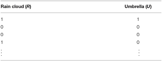
Table 1. Example observations of the presence of certain objects in a scene.
We might observe the following joint probabilities: From
the point of view of causal modeling, any particular distribution of data observed by a model is generated by physical, deterministic causal mechanisms (Parascandolo et al., 2018).
For our example, say that the underlying mechanisms that generate the data are as follows. Whether or not it rains depends on factors outside of the observed data (such as the humidity of the air, the temperature, etc.). Whether or not an umbrella is present depends on whether it rains as well as on factors outside of the observed data (such as the psychology of the people carrying the umbrellas, etc.) Let us collect these external factors in the variables ER for the rain cloud and EU for the umbrella. Then, the value of R is determined by the function R = fR(ER), and the value of U is determined by the function U = fU(R, EU). Because the model cannot observe ER and EU however, the best it can do is view them as random variables, and try to learn their distribution.
In this way, the probability distributions of the Ei, along with the causal mechanisms fi, generate a probability distribution of the observed variables: P(R, U). The set of observed variables and their relation is typically represented in an SCM. An SCM is a Directed Acyclic Graph (DAG) whose vertices consist of observed random variables X, Y, Z, … and in which a directed edge between nodes implies that the origin node is in the domain of the causal mechanism of the target node. Formally, if
then PAX is the set of variables with outgoing arrows into X.
Figure 1 shows the SCM for the example we discussed. Typically, the possible values and the unobserved variables are not explicitly shown, but we do so here for clarity.
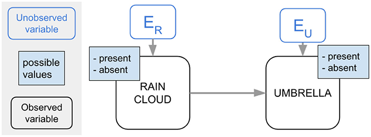
Figure 1. Example SCM.
To make the use of causality concrete for a visio-linguistic application, consider a model that needs to caption images. To do so successfully, it will need to recognize the different objects in the image. In order to recognize objects, the model will first of all make use of the per-object pixel-level information. However, to identify blurry, hard-to-recognize objects, it can complement that information with the context of the object. In other words, it can make use of knowledge about which objects are more or less likely to occur together. Consider the case where the image to be captioned is that of a rainy street. It is then useful for the model to be able to predict whether what it sees is a rain cloud given that it sees umbrellas (or vice versa).
A model that needs to learn parameters to perform this task can solve this in different ways. For instance, it could learn a parameter for each possible value of the joint probability P(U, R). This might be tractable for two variables, but for more variables, this approach requires too many parameters. Alternatively, it can learn a factorization of the joint probability and only learn parameters for each value of the factors. The two possible factorizations in this case are on the one hand P(U, R) = P(U|R)P(R), which is aligned with the underlying causal mechanism and on the other hand P(U, R) = P(R|U)P(U), which is not.
Each of these factorizations uses the same number of parameters, and each will be able to correctly answer queries like “what is the probability of not seeing umbrellas given that it rains.”
However, consider that there is a distribution change, for example, because we want our model to work for a location with more rain. In this case the factor P(R) has changed because of a change in the distribution of ER. To adapt, the factorization that was aligned with the underlying causal mechanism needs to change the parameter for only one factor, while the other factorization needs to change all its parameters.
Generalizing from this toy example, a distribution change typically only affects a few external factors Ei. Because of this, a model with a factorization that is aligned with the underlying causal mechanisms (a “causal” factorization Schölkopf, 2019) will typically need to update fewer parameters than a model with another (“entangled”) factorization, and thus perform well on out-of-distribution data with fewer modifications (Bengio et al., 2019).
Sometimes, we want to predict what setting the value of some variable X will have as an effect on the probability distribution of another variable Y, rather than what observing X will have as an effect.
Keeping Equation (1) in mind, “setting” a variable X to a value is the same as replacing the mechanism X = f(PAX, EX) that produces X with a constant X = x. Such an intervention to the underlying mechanisms then changes the resulting overall probability distribution. The distribution resulting from setting a variable X = x is indicated with the notation of the “do”-operator: the distribution of another variable Y in the SCM after we set (X = x) is noted as
Note the difference with the distribution of Y given that we observe X (rather than setting it):
An important case where the do-operator highlights the difference between observation and intervention is in the case of confounders. When two variables X and Y share a common parent Z in the SCM, this parent is called a confounder. The statistical dependence between X and Y is then (at least partly) attributable to this parent.
In the presence of a confounder, P(Y|X = x) will be different from P(Y|do(X = x)).
For example, consider the SCM in Figure 2. We might reasonably expect P(L = 1|U = 1) > P(L = 1|U = 0): the probability that a puddle is present increases given that we observe an umbrella. On the other hand, we should not expect that the probability of a puddle being present changes when we put an umbrella in a scene: P(L = 1|do(U = 1)) = P(L = 1|do(U = 0)) = P(L = 1).
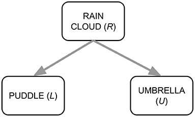
Figure 2. Example SCM.
The presence of a confounder can stand in the way of learning a causally aligned factorization. Consider again the SCM from Figure 2. The correct causal factorization is P(R, L, U) = P(U|R)P(L|R)P(R), but the correlation between puddle and umbrella might cause the model to use P(L|U) or P(U|L) as a factor. To discourage using these factors, we want to teach the model P(L|do(U)) (resp. P(U|do(L))) instead, as this spurious correlation disappears in the interventional view. In many domains however, such as the visio-linguistic domain, we cannot do actual real-life “interventions” on the data: we cannot “put” a rain cloud in a captioned image of a street and expect umbrellas to appear.
However, if we know the underlying SCM, we can still estimate P(Y|do(X)). To do so, we have to make sure that each confounder Zi is adjusted for. Intuitively, we want each confounder to be “homogeneous” (Pearl, 2009) with regard to X: we should take samples from the SCM in such a way that each Zi has the same distribution for every value of X. In this way, we “neutralize” any effect Zi might have.
For the example of Figure 2, if we want to discover whether there is a causal link between P and U, we want to compare the difference in how many times we see puddles for the case in which there is an umbrella present, with the case in which there is not, without being confounded by the effect of one case having rain more often than the other case. We do this by making sure there are as many rainy days for the case without an umbrella as for the cases with an umbrella.
More generally, there can be more than one confounder (e.g., if there are also sprinklers that cause people to take out their umbrellas and puddles to form), and each variable can have more than 2 possible values (e.g., if the variable is “color of the umbrella” rather than “presence of an umbrella.”) In this more general case, the “back-door criterion” tells us which set of variables SZ = {Z1, …, Zn} can be selected to be adjusted for to discover the causal link between two target variables X and Y: SZ is any set of variables such that:
• No node in SZ is a descendant of X;
• The nodes in SZ block every path between X and Y that contains an arrow into X.
Note that this means it is also possible to adjust for too many variables, creating a spurious correlation where there was none before adjusting, so simply adjusting for every variable will not work.
Formally, if each Zi ∈ SZ has ni possible values :
For example, for the case where there are only two confounders Z1 and Z2, each with only two possible values: absent (0) and present (1), Equation (6) becomes
This example is relevant as it applies to AutoDeconfounding, where variables are different objects, and their possible values are either “present” (1) or “absent” (0). The SCM assumed by AutoDeconfounding does not put restrictions on the connectivity between objects, as long as the resulting graph is a DAG. Moreover, it assumes no hidden confounders.
We will discuss the link of AutoDeconfounding with deconfounding in more detail in section 5.1, after first clarifying the details of AutoDeconfounding itself in section 4.
There are two variations of AutoDeconfounding: the one as implemented in VC-R-CNN (Wang et al., 2020), referred to as AD-V, and the one as implemented in DeVLBERT (Zhang et al., 2020b), referred to as AD-D.
Both Wang et al. (2020) and Zhang et al. (2020b) aim to improve on visio-linguistic tasks (e.g., Visual Question Answering or Image Captioning). Their models fall within a category of approaches that use transfer learning: They pretrain on a task different from the target task (a “proxy” task) for which more data is available (for example, context prediction or masked language modeling), and then fine-tune the resulting model on the actual downstream tasks of interest. Their innovation comes from an adaptation to the proxy task that is intended to prevent the model from learning spurious correlations.
VC-R-CNN and DeVLBERT differ slightly in both the context in which they use AutoDeconfounding and the exact implementation of AutoDeconfounding. This section will explain both models in detail.
The backbone of VC-R-CNN (Wang et al., 2020) is an image-region feature extractor [BUTD (Anderson et al., 2018)] which produces feature vectors for all regions-of-interest (ROIs) in an image. The image-region feature extractor is adapted by retraining it on a proxy task designed to prevent spurious correlations to be learned from vision data. Hence, VC-R-CNN focuses its contribution only on the image modality when pretraining.
During the pretraining, the loss function of VC-R-CNN consists of two terms:
The base objective Lbase,V is ROI classification, i.e., predicting the class of each of the N ROIs in the image. More precisely, if xi is the index of the class of the ith ROI and p is the vector of predicted probabilities computed based on feature vector fx extracted for the ith ROI, then the base objective is:
The additional objective LAD-V regards context prediction, i.e., predicting the class of one ROI based on the features of a different ROI in the image. It does this for each pair of ROIs in the image and sums the resulting losses:
where is a probability distribution over the possible ROI classes for the ith ROI computed based on feature vector fx of the context ROI to use for that prediction, yi is the index of the class of the ith ROI, and N is the number of ROIs in an image.
In order to predict the context in a “causal” way, VC-R-CNN introduces two elements that are gathered from the entire dataset: a confounder dictionary and prior probabilities .
The confounder dictionary is a set of C vectors, one per image class, where each consists of the average ROI feature of all ROIs in all images belonging to class c. Given fy and fx, where fy is the feature vector of the ROI whose class is to be predicted and fx is the feature vector of the context ROI to use for that prediction, VC-R-CNN computes a vector of attention scores α to select among those variables that are confounders for the classes corresponding to fx and fy. More precisely, the attention is computed as the inner product between fy and after projection to a shared embedding space, and converted to a probability distribution using softmax:
where α[c] denotes the element at the cth index in vector α, 〈·, ·〉 denotes the inner product, and with D the dimension of feature representations. In section 5.3, we use this α to investigate whether confounders are actually found.
Next, the model retrieves a pooled vector fz by taking a sum of each of the C vectors in weighted by both the attention score α[c] and the prior probability from :
Here, vector is a probability distribution over the classes according to how many images they occur in5. The weighting of by its prior is intended to realize the deconfounding. In section 5.1, we explain the exact link with deconfounding.
Finally, a simple feed-forward network FFN takes the concatenation of fx and fz and transforms it to the prediction over the possible classes :
where [·;·] denotes the concatenation operation. The pipeline for VC-R-CNN is shown in Figure 3.
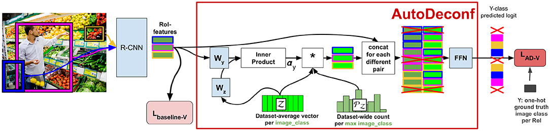
Figure 3. Pipeline for VC-R-CNN.
In order to clarify the analysis that we make in section 5.1, it is useful to rewrite . First, in Equation (13) we can write the feed-forward network FFN as the function gV:
Second, in Equation (12) assume that each α[c] were to perfectly select confounders (i.e., if there are c true confounders, give each of those c true confounders a weight of 6, and all other variables a weight of 0). Use Sz to denote the set of c indices of vectors in for which the corresponding class is a confounder for the classes corresponding to fx and fy. Then, we can summarize as:
Note that in the case where c > 1, the softmax from Equation (11) will tend to promote the selection of one confounder, even if there are multiple attention scores that are quite high in the input of the softmax.
To deal with the case of multiple confounders, a sigmoid function, subsequently scaled so that the entries still sum to one, would have been a better choice. However, as Zhang et al. (2020b) and Wang et al. (2020) use a softmax for AutoDeconfounding, we will consider the softmax in our further analysis.
VC-R-CNN uses image datasets with ground truth bounding boxes [MS-COCO (Lin et al., 2014)] and Open Images Kuznetsova et al., 2020). The regions within these bounding boxes are the ROIs.
VC-R-CNN aims to improve performance on Image Captioning (IC), Visual Commonsense Reasoning (VCR) (Zellers et al., 2019) and Visual Question Answering (VQA) (Antol et al., 2015). More precisely, the image features extracted with VC-R-CNN are used as part of the pipeline of the various downstream models7.
DeVLBERT (Zhang et al., 2020b) uses the exact same backbone and modalities as ViLBERT (Lu et al., 2019). Like ViLBERT, it uses a Faster R-CNN region extractor (Ren et al., 2015) [with ResNet-101 (He et al., 2016) backbone] to convert images into sets of region features, and initializes the weights for the linguistic stream with a BERT language model pretrained on the BookCorpus and English Wikipedia. It also adds the same cross-modal parameters.
Just like ViLBERT, DeVLBERT then performs visio-linguistic pretraining. The only difference is that it adds a number of “causal” parameters and losses during this pretraining, intended to make the model less prone to spurious correlations. These are detailed in the rest of this section. When the model is finetuned for downstream tasks, these extra parameters are no longer used: their only purpose was to change the “non-causal” parameters.
During the pretraining, the loss function for DeVLBERT is:
DeVLBERT's base objective equals the one described in ViLBERT (Lu et al., 2019) which consists of a masked token modeling loss for each modality (LMTMV and LMTMT), and a caption-image-alignment prediction loss (LVLA):
DeVLBERT's additional objective is similar to that of VC-R-CNN, but then extended to the multi-modal setting. More precisely, DeVLBERT predicts the class index yi of the ith token (where “tokens” are words for the text modality, and ROIs for the vision modality) based on the contextualized feature fy for that same token. This means LAD-D consists of 4 loss terms:
where t stands for the text modality and v for the vision modality. Similar as in VC-R-CNN, a cross-entropy loss is used for the loss terms. For example, is computed as:
where is the class index of the ith textual token, and the prediction over the possible classes for the ith textual token is computed using the confounder dictionary for the vision modality. The computation of the other loss terms is completely analogous.
The pipeline for DeVLBERT is shown in Figure 4.
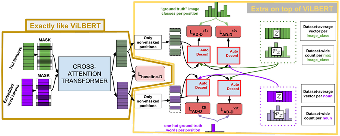
Figure 4. Pipeline for DeVLBERT.
Note that Figure 4 only describes variation “D” of the variations proposed in DeVLBERT, as this is the variation for which most results were reported in Zhang et al. (2020b).
Since DeVLBERT does AutoDeconfounding in the multi-modal setting, one of the main differences compared to VC-R-CNN is that modality-specific confounder dictionaries and and modality-specific prior probabilities and are used to do the context prediction in a “causal” way. In the following, we describe the pipeline for the text-to-vision case only, but the other cases are completely analogous.
In the text-to-vision case, for the context prediction of a textual token with feature vector the confounder dictionary for the visual modality is used. First, attention scores α are calculated to select among the visual tokens in those that are confounders for the textual token represented by . Next, a pooled is calculated by weighting the C vectors in confounder dictionary based on the attention score α[c] and prior frequency :
where α[c] denotes the element at the cth index in vector α, 〈·, ·〉 denotes the inner product, and with D the dimension of feature representations. In section 5.1, we explain the exact link of weighting by its prior with deconfounding. Furthermore, in section 5.3, α is used to investigate whether confounders are actually found.
Another main difference with VC-R-CNN is the input for the prediction, which is not a concatenation, but only the pooled vector :
Figure 5 shows a zoom-in of the AutoDeconfounding operation in DeVLBERT (Equations 21–23). Note that for DeVLBERT, the ROI feature vector fy that is used to do the prediction (by selecting fz as an intermediate step), and the class yi that we want to predict, actually correspond to the same token. In other words, DeVLBERT is finding variables that are confounders for the same variable. Zhang et al. (2020b) justify this by saying fy actually corresponds to a “mix” of tokens, since it has been contextualized through the self-attention mechanism in the ViLBERT backbone. However, this contextualization does not take away that fy mainly corresponds to the token in the image with class yi. In the three-way relation of a confounder, if the two variables X1 and X2 that are confounded by variable Z are one and the same (X1 = X2 = X), we can simply call Z a cause of X. Figure 6 illustrates this. We can thus also speak of “causes” instead of “confounders” when discussing DeVLBERT.
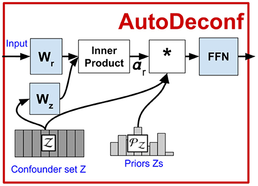
Figure 5. Zoom-in of AD-D.
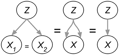
Figure 6. Three-way confounding relations collapsing to a two-way causal relation.
Again, we can rewrite into a form suitable for the analysis in section 5.1. First, we write the feed-forward network FFN as the function gD:
Second, we simplify by assuming that each α[c] perfectly selects confounders (or in this case: causes) and that Sz is the set of c indices of vectors in for which the corresponding class is a cause for the class corresponding to . Then, we can summarize as:
DeVLBERT uses a dataset of images paired with captions [Conceptual Captions (Sharma et al., 2018)]. We refer to an image-caption pair as a “record.” DeVLBERT does not use the images directly though, but uses a frozen region feature extraction network [BUTD (Anderson et al., 2018)] to represent the images as sets of ROI features. Note that for images, DeVLBERT does not use ground truth bounding boxes (as those do not exist for Conceptual Captions), but takes the predictions of the frozen and pretrained BUTD region proposal network as approximate ground truth.
For DeVLBERT, the downstream tasks are VQA, Image Retrieval (IR) and Zero-Shot Image Retrieval (ZSIR). Specifically, they train and evaluate VQA on the VQA 2.0 dataset (Antol et al., 2015) consisting of 1.1 million questions about COCO images (Chen et al., 2015), each with 10 correct answers, and (ZS)IR on the Flickr30k dataset (Young et al., 2014) consisting of 31 000 images from Flickr with five captions each. They exactly follow the splits and training setup of ViLBERT for this, as do we in the experiments described in the next section. Note that when applied to downstream tasks, DeVLBERT has the same architecture as ViLBERT: the only difference is that its weights are different due to the different pretraining objective (Equation 17).
The DeVLBERT authors argue that there is a distribution shift between the pretraining data (Conceptual Captions) and the data of downstream tasks (VQA 2.0 and Flickr30k), namely because the captions in Conceptual Captions are automatically extracted based on alt-text attributes, whereas the VQA and Flickr30k captions are human-annotated. This is in line with other works on multi-modal pretraining that also consider Conceptual Captions to have no expected overlap with the data of common downstream tasks (Bugliarello et al., 2021). As explained in section 3.2, a model that makes prediction using only correlations that are also causal, should be expected to better adapt to a distribution shift.
Note that DeVLBERT uses the same region proposal network and text tokenizer for pretraining and downstream tasks. This means that the distribution is not different in which object or token classes appear, but rather in the statistics of the appearance of the same set of object or token classes.
To investigate the reported improvements of DeVLBERT, we copy their out-of-distribution setting. However, for future work, it can be interesting to consider a setting where the distribution shift is more explicit. For example, a distribution shift where certain classes are known to have different correlations.
The previous sections provided background knowledge of causality and of AutoDeconfounding. This section will build upon that knowledge to examine AutoDeconfounding more closely.
Our methodology for investigating AutoDeconfounding consists of three parts: one theoretical analysis, and two empirical investigations for which we retrain a number of variations of the SOTA model that uses AutoDeconfounding. First, we theoretically examine whether the implementation of AutoDeconfounding actually corresponds to deconfounding. Second, we evaluate performance on downstream tasks to isolate which component of AutoDeconfounding is responsible for the reported improvements on those tasks. Finally, we examine to what extent confounders are actually found. We develop a ground truth dataset of causal relations to investigate this quantitatively, and qualitatively show a subset of the most-selected confounders.
The implementation of AutoDeconfounding was detailed in section 4. In this section, we explain how that implementation relates to the formula for a deconfounded prediction (Equation 6). We show the derivation as made in VC-R-CNN and DeVLBERT, and expand it to clarify the link with the underlying causal model.
The derivation starts with the formula for deconfounding:
As explained in Equation 6, this is really a simplified notation for
where vx and vy each can be either 0, meaning “absent from the scene” or 1, meaning “present in the scene,” and {Z1…ZC} is the set of classes that form a confounder for X and Y. For simplicity of notation, we rewrite
as
The derivation in VC-R-CNN and DeVLBERT then shows that P(Y = vy|X = vx, Z1 = vz1, …, Zc = vzc) is calculated with softmax(g(fx, fz)). Equation (28) then becomes:
Note that this implies that the state of X is encoded in fx, and the joint state of Z1, …, Zc is encoded in fz.
The derivation then makes an approximation to move Ecz into the softmax following the idea of the Normalized Weighted Geometric Mean, or NWGM. The idea of NWGM is similar to that of how dropout approximates an ensemble of models. It approximates the aggregate result of resampling (in multiple passes) cases where X = vx so that Z occurs at the rate P(Z = vz) by 1) only doing one pass for X = vx, but 2) using the NWGM of the possible values vz of Z, weighted by their prior distribution P(Z = vz).
Further, given that the function g(·, ·) is linear, the expectation can be moved next to the argument fz:
Writing 𝔼cz in full again:
we can now compare this with the actual implementation as explained in section 4 in Equations (16) and (26).
First, specifically for DeVLBERT (Equation 34), there is a mismatch in the first argument of g: fx is no longer involved for gD, meaning that the prediction is made based on only the state of the confounder variables.
Second, for both VC-R-CNN and DeVLBERT, there is an apparent mismatch in the second argument of g. Equation (32) shows that the sum should be taken over all possible combination of values for every possible confounder. However, in the actual implementation, Equations (33) and (34) show that the there is only one term per confounder, corresponding to the case where its value is “present.”
For example, if Y is puddle, X is umbrella, Z1 is rain cloud and Z2 is sprinkler, then there are two confounders for P(Y|X): Z1 and Z2. Instead of calculating P(Y|do(X)) by taking the average value of P(Y|X, Z1, Z2) weighted by the prior probabilities P(Z1 = present, Z2 = present), P(Z1 = present, Z2 = absent), P(Z1 = absent, Z2 = present), P(Z1 = absent, Z2 = absent), AutoDeconfounding takes the average value weighted by the prior probabilities P(Z1 = present), P(Z2 = present).
Despite this apparent mismatch, with two additional assumptions that were not specified in Zhang et al. (2020b) or Wang et al. (2020), it is possible for this second argument of g from Equation 32 to simplify into matching the second argument of g in Equations (33) and (34):
For the first assumption, note that in the implementation, the joint state Z1, …, Zc is encoded as follows: For each Zi, if its state is “present,” it is represented by the average ROI feature vector fzi of the corresponding class. These average vectors are the ones collected in the confounder dictionary . If its state is “absent,” it is represented by a zero-vector with the same shape as fzi. Then, the joint state is represented as the average vector . The assumption is then that fz can successfully distinguish all possible joint states.
The second assumption is that all the confounders are independent of one another. This entails that .
Under these two assumptions, it can be shown that terms of the sum in Equation (32) reduce (barring scaling factors) to the terms in the implementation Equations (33) and (34). The proof for this is in Appendix section 1.1.
In conclusion, we show that certain additional assumptions are needed to overcome the mismatch between theoretical deconfounding on the one hand, and the implementation of AutoDeconfounding on the other hand. More specifically, it is necessary to assume that the various confounders are independent of one another, and that the encoding of the joint confounder state as implemented in AutoDeconfounding can uniquely determine each state.
In the next sections, we evaluate aspects of AutoDeconfounding empirically. We perform our empirical experiments only for DeVLBERT, as it is the state-of-the-art of this articles that use AutoDeconfounding.
As explained in section 4.2, Zhang et al. (2020b) evaluate the quality of the DeVLBERT model by its performance on downstream visio-linguistic tasks. They report a significant improvement on these tasks when extending their baseline model with AutoDeconfounding.
Our analysis from section 5.1 shows that additional assumptions are necessary to equate the implementation of AutoDeconfounding with deconfounding. Inspired by this, we perform ablation studies to verify to what extent deconfounding is actually responsible for the reported improvement in scores. We do this by adapting AutoDeconfounding in such a way that it retains access to the confounder dictionary, but is no longer related to deconfounding. We also verify the extent of the contribution of AutoDeconfounding as a whole, by comparing with a baseline that does not use AutoDeconfounding on a more like-for-like basis.
Because we want to investigate the relation between the implementation of AutoDeconfounding and the performance increase on downstream tasks as reported by DeVLBERT, we evaluate on exactly the same downstream tasks as DeVLBERT.
For our first experiment on downstream task performance, we test the hypothesis that the key ingredient is the use of the “confounder” dictionary . We hypothesize that forces contextualized representations to be sufficiently close to a per-class average representation, thus providing some kind of regularization. In this hypothesis, is an irrelevant component of AutoDeconfounding. To isolate the effect of , we have implemented and trained-from-scratch two variations of AutoDeconfounding for which we alter .
First, we create a model named DeVLBERT-NoPrior in which is left out completely. This changes Equation (22) to:
Second, we create a model named DeVLBERT-DepPrior in which is replaced by a dependent prior. As opposed to vanilla DeVLBERT, DeVLBERT-DepPrior does not weight each entry in by the prior frequency of the class corresponding to that entry. Rather, it takes into consideration both the class Cz of the entry in the confounder dictionary , and the class Cy of the token that is being predicted. It weights each entry by the frequency of tokens of class Cz within records of the Conceptual Captions dataset where a token of class Cy is also present.
Because DeVLBERT has a loss term for each combination of modalities, DeVLBERT-DepPrior has a dependent prior for each modality combination. For example, the dependent prior used to calculate the loss term is:
Where T is the total number of records, j and k denote the class indexes for modality t and v, respectively, and It(j, k) is an indicator function that is 1 if modality t of the jth record contains a token with class index k and 0 otherwise.
Equation (22) then becomes:
where i is the index of Cy and c the index of Cz.
If these variations achieve a similar score to DeVLBERT, that supports the hypothesis that is the key component of AutoDeconfounding.
For our second experiment on downstream task performance, we observe that the comparison between DeVLBERT and ViLBERT in Zhang et al. (2020b) is not made on a completely like-for-like basis, and so does not properly isolate the effect of AutoDeconfounding.
More specifically, DeVLBERT was trained for 24 epochs, where for the last 12 epochs the region mask probability is changed from 0.15 to 0.3 (Zhang et al., 2020b), whereas ViLBERT is only trained for 10 epochs (with region mask probability 0.15)(Lu et al., 2019). Zhang et al. (2020b) report that longer pretraining can be especially beneficial for zero-shot IR performance8. Moreover, for fine-tuning, ViLBERT uses the last checkpoint for evaluation, whereas DeVLBERT uses the best checkpoint (based on the validation score) for evaluation.
We retrain and ViLBERT and DeVLBERT ourselves on a like-for-like basis. The details of our experimental setup are in section 6.1.
The last question we investigate is whether confounders are actually found. According to the Causal Hierarchy Theorem (Bareinboim et al., 2020), with access to only observational data, you cannot make a model that correctly answers interventional (causal) queries for “almost-all9” underlying SCMs. Or as stated by Cartwright (1994): “no causes-in, no causes-out.” Moreover, Zhang et al. (2020b) and Wang et al. (2020) did not quantitatively verify whether confounders are found, but take this as a given. Taking the above into account, it is not obvious that confounders are actually found by AutoDeconfounding.
We evaluate the confounder-finding capacities of DeVLBERT both quantitatively and qualitatively. Because we focus on DeVLBERT, we will speak of “causes” instead of “confounders.”
A lot of the tokens from the text modality are not meaningful as causal variables (words such as “over,” “the,” etc.) Hence, we focus specifically on the image modality, where all of the tokens correspond to real objects.
To check quantitatively whether actual causes are found, we need ground truth labels on the causality between objects in a scene.
To do this, we create a novel dataset with ground truth labels. Ideally, the way to gather causal labels would be to do interventions in the real world. However, this is difficult to realize (e.g., it is hard to “put” a rain cloud into a scene). Because many causal relations between objects are obvious to human common sense, we rely on human judgement to annotate causal relations instead. The assumption here is that the “mental intervention” that humans do when they answer a question like “Would changing the presence of ‘umbrella’ influence the presence of ‘rain cloud’ in the scene?” is a good approximation of the real-world intervention.
Selecting Data to Label DeVLBERT works with 1,600 visual object classes, so the number of class-pairs for which a causal-link question can be asked is 1, 6002 = 2.56 million pairs. Because we believe most of these pairs will have no direct link at all, and labeling all 2.56 million pairs is too expensive, we select a subset of 1,000 class pairs to label. To select this subset, we use the following heuristic:
We assume that candidate pairs that are not correlated in the dataset, will not exhibit a causal link either10. Hence, to select a subset of pairs, we ranked pairs by how strongly they were correlated in the dataset. More specifically, if P(X = 1) is the probability that an image contains an object of class X, and P(X = 1, Y = 1) is the probability that an image contains both an object of class X and an object of class Y, we select classes for which the difference between P(X = 1, Y = 1) and P(X = 1)P(Y = 1) is large.
We select 500 class pairs for which the absolute difference |P(X = 1, Y = 1)−P(X = 1)P(Y = 1)| is the highest, and 500 pairs for which the relative difference log(P(X = 1, Y = 1)/P(X = 1)P(Y = 1))11 is the highest12.
Assuring Label Quality. To label the data, we used Amazon Mechanical Turk (MTurk)13. We ask workers to label pairs (X,Y) of correlated objects with one of three options: X causes Y, Y causes X, or neither (in other words some confounder Z causes X and Y). In the latter case, we also provide a free-form box where workers could enter what they thought this confounder would be. An example of the form we used can be found in the Supplementary Material. We also let workers fill in a confidence score of 1–3 of how confident they are in their answer.
The kind of causality that we target is non-trivial to non-experts: we say that one object “is the cause of” another if intervening on its presence influences the probability of the other object being present. To ensure that workers understand the task well, we provide detailed instructions in the form, along with an explanation video. We also require that workers get a minimum score on a test with a small number of pairs with an obvious causal direction. The test questions can be found in the Supplementary Material.
We let each pair be labeled by 5 different workers and keep only those pairs for which agreement was at least 4 out of 514. This left us with 595 pairs (or about 60 percent of pairs with at least 4/5 agreement). Table 2 shows 10 of these pairs.
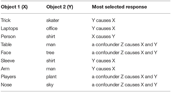
Table 2. Subset of response pairs from crowdworkers.
Table 3 shows some examples of confounders that workers entered in the free-form box. One pattern to observe is that when the two objects are parts of a whole, the whole is sometimes suggested (e.g., windshield wipers and doors are caused by a car, or outfield and mound by baseball field). Suggested confounders can also vary quite widely (e.g., table, office, or coffee shop as confounder for coffee cup and monitors).
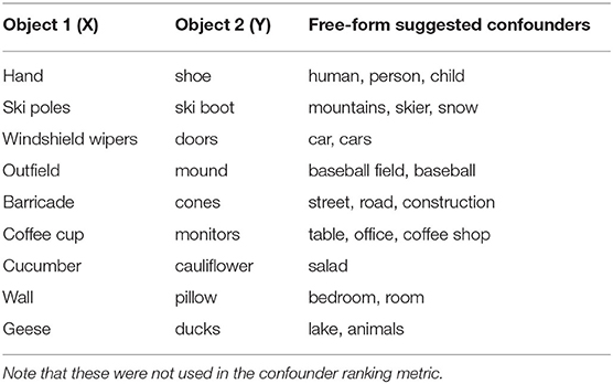
Table 3. Subset of free-from confounders suggested by crowdworkers.
The full dataset with responses, confidences and free-text confounder responses is publicly available on Google Drive15.
Recall from Equation 22 that the mechanism by which causes are found consists of using attention scores α to pool vectors from whose classes correspond to causes.
We take the trained model from DeVLBERT, and for every ROI y in every image, we produce α. We then examine the objects classes oi in our dataset for which we have the ground truth relation to y (i.e., either oi is a cause of y, y is a cause of oi, or they are “mere correlates.”) We call the set of oi for a particular y Oy. A successful α should rank the oi that are a cause of y higher than the oi that are either consequences or mere correlates. We use mean average precision (mAP) as metric to measure the ranking performance. We compare the resulting mAP score with a baseline that ranks the elements of Oy in a completely random way.
We report on the results in section 6.2.1.
The quantitative analysis only considers classes for which we have collected ground truth causality information. It can be informative, however, to look at the complete ranking of candidate causes for a certain class.
We calculate the per-class average value of α[c] over all R ROIs in the dataset whose ROI class corresponds to c for each class c:
where is the contextualized ROI-feature corresponding to the ith ROI, is the confounder dictionary for the image modality, and I(i, c) is an indicator function that is 1 if the ith ROI has class c and 0 otherwise.
We also show a few qualitative examples during a downstream task, specifically VQA. We check the last-layer cross-modal attention from a query word in the question to the bounding box of an object which we know is a cause of the query word. This can indicate whether certain models pay more attention to actual causes during downstream tasks.
As explained in section 4.2, Zhang et al. (2020b) evaluate the quality of the DeVLBERT model by its performance on three downstream visio-linguistic tasks: Image Retrieval and Visual Question Answering, for which the model is further fine-tuned, and Zero-Shot Image Retrieval, for which the pretrained model is immediately used. Performance on (Zero-Shot) Image Retrieval is measured by recall at k or R@k, and performance on Visual Question Answering is measured by accuracy. We evaluate in the same way.
When reproducing DeVLBERT, we have tried to follow the original setup as closely as possible. We train all models with the same batch size and learning rate as DeVLBERT16.
There are, however, still a few differences in set-up. First, for Visual Question Answering, we only report performance on the “test-dev” split, and not on the “test-std” split: only 5 submissions to “test-std” are allowed, and we evaluate more than 5 models. Second, because the Conceptual Captions dataset consists of hyperlinks to web content, over time some of the links go stale. Hence we work with 2.9 million records, compared to the 3.1 million that DeVLBERT originally trained on.
Finishing 24 epochs of pretraining on the Conceptual Captions dataset takes 3–5 days17.
A pretrained checkpoint was made publicly available by Zhang et al. (2020b). We redo only the fine-tuning step ourselves for this checkpoint, and also include its performance in our results. We refer to this run as DeVLBERT-CkptCopy.
To make sure that the improvement is indeed due to AutoDeconfounding, we retrain ViLBERT and DeVLBERT ourselves, this time in exactly the same way: both for 24 epochs, where for the last 12 epochs the region mask probability is changed from 0.15 to 0.3, and both using the best checkpoint in the fine-tuning tasks for evaluation.
Table 4 shows an overview of the downstream tasks performances of the different models we evaluated18.
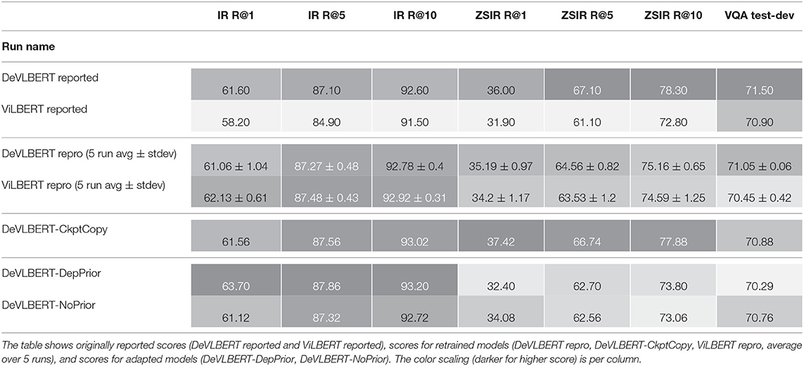
Table 4. Scores on downstream tasks: top-1 recall, top-5 recall and top-10 recall for Image Retrieval (IR R@1, IR R@5, IR R@10) and zero-shot image retrieval (ZSIR R@1, ZSIR R@5, ZSIR R@10), and accuracy on the test-dev split for Visual Question Answering (VQA).
We make a couple of observations:
The top two rows show the improvement of DeVLBERT over ViLBERT as reported in Zhang et al. (2020b). The next two rows show the same comparison, but for our like-for-like reproduction where we retrained DeVLBERT and ViLBERT from scratch. Contrary to Zhang et al. (2020b) we do not observe an improvement across the downstream tasks. Part of the gap is closed by the better score of ViLBERT. Especially on IR and ZSIR, we see that training for more epochs improves the R@1 for ViLBERT by almost 2 to 3 percentage points. This indicates that the reported improvement in Zhang et al. (2020b) might be largely due to differences in training, rather than due to AutoDeconfounding.
However, another part of the difference between the reported scores and our reproduces scores is that we get a lower score than reported for DeVLBERT in our reproductions. As we use the code provided by Zhang et al. (2020b) to retrain models, we hypothesize that this difference is due to the slightly smaller size of the pretraining dataset that was available to us.
We see that DeVLBERT-CkptCopy scores are different from the reported scores. This is because the model checkpoint that the authors of DeVLBERT made available is not the one for which they reported results19.
Although we could not quite reproduce the results in the same way, our results indicate that the reported improvement in Zhang et al. (2020b) might be mainly due to a different training regime.
Finally, the results for DeVLBERT-DepPrior and DeVLBERT-NoPrior do not show a consistent degradation of performance on all downstream tasks when compared to DeVLBERT repro. This indicates that the component of AutoDeconfounding indeed is not a key component.
All in all, these results cast serious doubt on the validity of AutoDeconfounding as a method to improve performance on out-of-domain downstream tasks.
For the experiments that investigate confounder finding, we only evaluate runs that are variations of DeVLBERT, but not runs that are variations of ViLBERT. ViLBERT does not contain the mechanism that selects confounders, shown in Equation (21), and so cannot be judged on whether it finds confounders. More specifically, we evaluate DeVLBERT repro, DeVLBERT-CkptCopy, DeVLBERT-DepPrior, and DeVLBERT-NoPrior.
Table 5 shows the mAP results.
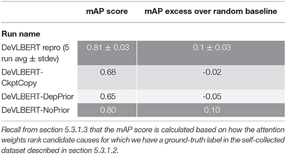
Table 5. Comparison of confounder-finding performance of DeVLBERT with a random baseline.
Table 5 shows that the reproduced runs behave differently than DeVLBERT-CkptCopy. Whereas DeVLBERT-CkptCopy is worse than random at correctly ranking the causes in the ground truth dataset, the reproduced runs score better than random. We trained multiple reproductions to see whether this was due to high variance for the mAP score over different initializations, but this behavior holds up over 5 runs. Recall from section 6.1 that the reproduced model scores slightly lower than DeVLBERT-CkptCopy on downstream tasks. This indicates that finding or not finding confounders does not correlate with performance on the downstream tasks.
Further, for DeVLBERT-DepPrior and DeVLBERT-NoPrior, we get mixed results. DeVLBERT-NoPrior shows a similar result to the reproduced runs, while DeVLBERT-DepPrior again shows a worse-than-random result. Given the Causal Hierarchy Theorem mentioned in section 2, we might expect that it would not be possible to correctly identify causes given only observational data, and so we would expect all runs to score around the random baseline. We propose the following explanation for this apparent paradox. While the CHT states that the correct SCM cannot be recovered from only observational data, it can be recovered up to its Markov Equivalence Class. We hypothesize that for the ranking task we developed, this might be sufficient to score above-random. We hypothesize that a more specialized ranking task that explicitly seeks to test cause-finding beyond what can be deduced up to the level of a Markov Equivalence Class will be harder. Performance on such a harder confounder-finding task might then be a better predictor of out-of-distribution performance. We leave the development of such a task for future work.
In conclusion, we get mixed results in trying to evaluate ground truth confounder-finding, however the results do indicate that confounder-finding ability does not correlate with performance on downstream tasks.
For the qualitative investigation of confounder-finding, we do not average the result of DeVLBERT repro, but show the result for only one of the runs. Because different runs might produce a different ranking, it is hard to display the average results in a compact way. Because it is a qualitative investigation, the result for a single run is sufficiently informative. We display the run with the best mAP score.
The full 1600 × 1600 tables with the attention distributions can be found in the Supplementary Material. The scores shown are the values of α[c] in Equation (21), averaged over all records containing the effect variable. Table 6 shows a subset, that is, the top ranked classes for the 10 most common objects.
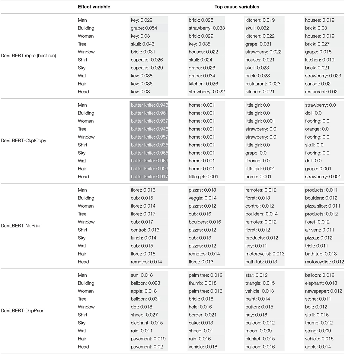
Table 6. The average top predicted “causes” in the confounder dictionary and the corresponding average attention score α[c] for the 10 most common objects (in bold in the leftmost column).
Table 7 shows the same values, but for a particular example of each effect variable rather than for the average20.
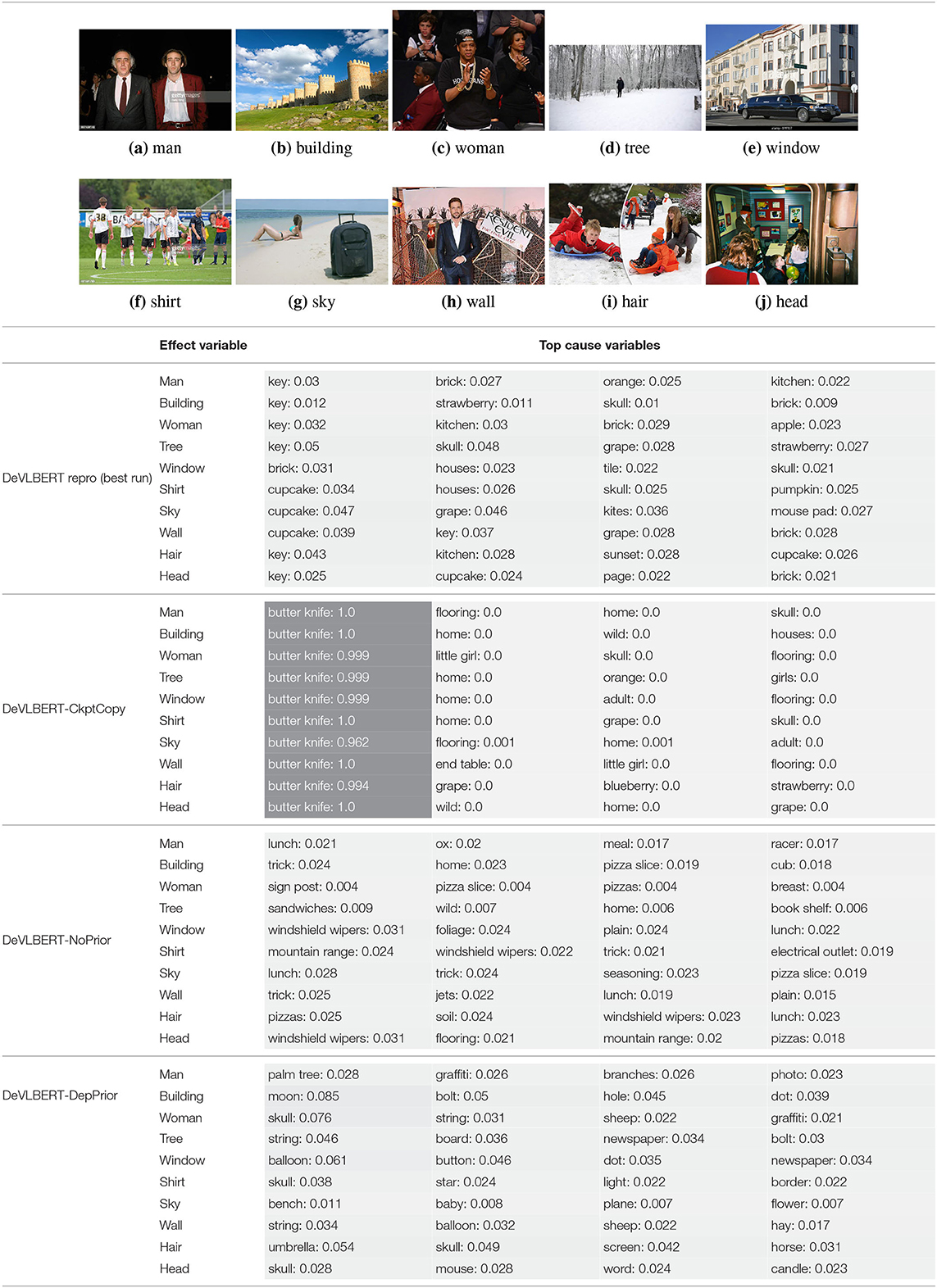
Table 7. The top predicted “causes” in the confounder dictionary and the corresponding attention score α[c], not averaged over all images as in Table 6, but for the objects detected in the specific images shown above.
For DeVLBERT-CkptCopy, the by-far most-attended-to element of the confounder dictionary is “butter knife,” and the rest of top-attended elements are similar between objects. For the other runs, there is no one most-attended-to element, but we also see a small set of classes appearing as top-cause candidates for different effect variables.
To explain the high-confidence “butter knife”-selecting behavior, we hypothesize that DeVLBERT-CkptCopy found a beneficial local optimum that makes use of in a specific way. The low-confidence predictions for the other runs then indicate that they did not find such an optimum.
It does not seem to be the case however that either case corresponds to finding actual confounders. For DeVLBERT-CkptCopy, it seems unlikely that “butter knife” is indeed the most likely confounder for every class. The top causes selected by the other models also do not seem intuitively causal: “key” causing “man” for DeVLBERT repro, “cub” causing “building” for DeVLBERT-NoPrior, or “apple” causing “woman” for DeVLBERT-DepPrior do not seem related to true causality.
The fact that the same classes appear as top causes for unrelated effect variables indicates an indifference of the model to the value of the effect variable: Which cause variable receives a large attention score, depends more on the value of the particular (fixed) embedding for that cause variable, than on how well it matches with the effect variable for which a cause is supposedly found. Note that the cause variable representation comes from the (fixed) confounder dictionary, whereas the effect variable representation is the contextualized output of the Transformer model. We hypothesize that this asymmetry is due to the projection matrices that precede the inner product in the calculation of attention scores. The model might have found it beneficial to make the weights in these projection matrices such that the attention output is more related to the cause variable than to the effect variable.
Note that the attention parameters in AutoDeconfounding are never explicitly trained to make confounder-finding predictions. Rather, it is assumed by AutoDeconfounding that the attention scores can be interpreted as cause-selecting-scores. The selection of top causes observed in Table 6 indicates that this interpretation is not valid.
Table 8 shows a few example images of a downstream task (VQA), where the query word is an effect, and the bounding box shown is that of a cause. If a model learned to depend less on spurious correlations and more on causes during pretraining, it is expected that this is reflected in higher attention values from effects to causes. We do not observe that the models using variations of AutoDeconfounding pay significantly more attention to the cause object than the baseline ViLBERT model.
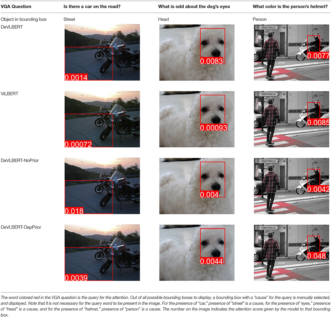
Table 8. Some examples of the attention from query word to cause bounding box, for different models.
Models relying on spurious correlations are an important issue, and leveraging causal knowledge to address the issue is a promising approach. Causal models benefit transfer learning, allowing for faster adaptation to other distributions and thus being more generalizable (Schölkopf, 2019). This has been a popular approach to tackle spurious correlations specifically in the visio-linguistic domain, where a number of works have used it to further improve on the already impressive representation-learning capacities of Transformer-like models.
Leveraging causality with automatically discovered causal structure is especially interesting, as it could scale much better than human-labeled causal structure. This critical analysis has uncovered some of the issues with this approach.
First, care needs to be taken in being specific with regard to the underlying causal model that is assumed. As shown in section 5.1, only when making the link between causal variables and data-representations explicit is it possible to specify the assumptions under which an implementation of deconfounding is valid. An interesting avenue for future work could be to adapt the implementation to work with a less strict set of assumptions. Furthermore, more thought should be given to the design of models that produce interpretable representations that provide insight in the causal structure and relations of objects captured by these models. It would also be insightful to validate whether the assumptions hold for the application of interest.
Second, it is important to isolate the effect of causal representation learning: as section 5.2 shows, when doing a like-for-like comparison, in which the baseline is reproduced under the same circumstances, it is important to avoid confusing the effect of training circumstances with those of the added loss. Moreover, it is crucial to ablate every component to verify to what extent it is responsible for the improvement of the whole. Specifically for out-of-distribution applications, it would be interesting to discover which spurious correlations change between the distributions of interest, and whether those have been correctly captured by the model.
Finally, a key element in leveraging causality with automatically discovered causal structure is assessing to what extent the discovered structure is accurate. Our investigation using human-proxy-for-ground-truth shows mixed results in this regard, with the models that perform better on downstream visio-linguistic tasks scoring worse than random in a cause-ranking task. First testing models on domains for which the causal structure is known, for instance, as done by Lopez-Paz et al. (2017) can help to build confidence in the fact that causal operations such as deconfounding are realized using the correct causal model.
For future work, creating more extensive causally annotated datasets can enable progress in causal discovery. Additionally, it can be interesting to explore causal models that are more fine-grained than object co-occurrence, as spurious correlations are present at the level of objects as well as the level of object attributes. For example, taking attributes as causal variables, or making use of temporal data such as videos. More fine-grained variables can also be expected to be useful for novel distributions with unseen objects: if the unseen objects consist of known “parts,” their causal properties could still be predicted.
The datasets presented in this study can be found in online repositories. The names of the repository/repositories and accession number(s) can be found in the article/Supplementary Material.
NC came up with the idea to critically investigate AutoDeconfounding, conducted the experiments, created the figures, and was the main contributor to the text. KL and M-FM provided useful insights and suggestions during meetings, and provided suggestions and corrections for this article text during writing. All authors contributed to the article and approved the submitted version.
This research was financed by the CALCULUS project—Commonsense and Anticipation enriched Learning of Continuous representations—European Research Council Advanced Grant H2020-ERC-2017-ADG 788506, http://calculus-project.eu/. KL was supported by a grant of the Research Foundation—Flanders (FWO) no. 1S55420N.
The authors declare that the research was conducted in the absence of any commercial or financial relationships that could be construed as a potential conflict of interest.
All claims expressed in this article are solely those of the authors and do not necessarily represent those of their affiliated organizations, or those of the publisher, the editors and the reviewers. Any product that may be evaluated in this article, or claim that may be made by its manufacturer, is not guaranteed or endorsed by the publisher.
The authors would like to acknowledge the Vlaams Supercomputer Centrum for providing affordable access to sufficiently powerful hardware to perform the needed experiments in a reasonable timeframe.
The Supplementary Material for this article can be found online at: https://www.frontiersin.org/articles/10.3389/frai.2022.736791/full#supplementary-material
1. ^Intuitively, intervening on the value of some variable (like the presence of an object in a scene) means manipulating its value independently of the value of all other variables. This is defined formally in section 3.3.
2. ^For example, the correlation observed between umbrellas in the street, and number of taxis being taken is not due to a direct causal link, but due to the common cause of rainy weather.
3. ^Also Structural Equation Model.
4. ^The set of SCMs that encode the same set of conditional probabilities.
5. ^Note that the way is normalized implies that if every class would appear in every image, each class would have a value of in rather than a value of 1.
6. ^Note that because a softmax is used to calculate the attention score, it is not possible to give more than one confounder a weight of 1.
7. ^Up-Down (Anderson et al., 2018) for captioning and VQA, AoANet (Huang et al., 2019) for captioning, MCAN (Yu et al., 2019) for VQA, R2C (Zellers et al., 2019) and ViLBERT (Lu et al., 2019) for VCR.
8. ^See DeVLBERT replication instructions at https://github.com/shengyuzhang/DeVLBert.
9. ^“Almost-all” is meant in a measure-theoretic sense, explained in Bareinboim et al. (2020).
10. ^Although correlation is not a necessary condition for causation, for this heuristic we assume this is still a useful way to weed out many uninteresting pairwise relations.
11. ^We do not use the absolute value of log(P(X = 1, Y = 1)/P(X = 1)P(Y = 1)) because this fills the top of the ranking with pairs of classes that occur only once but not together: for these pairs, log(P(X = 1, Y = 1)/P(X = 1)P(Y = 1)) is minus infinity. These pairs are almost all unrelated and thus not causally meaningful.
12. ^The absolute difference surfaces more common classes, while the relative difference also surfaces rare classes.
13. ^We detail the crowdworkers' reward per label and estimated time spent per label in the Ethical Considerations section at the end of this article.
14. ^We did not end up weighting agreement by confidence level as the difference in resulting pairs was small anyway.
15. ^https://drive.google.com/file/d/17CTPMoZ4uJH6cSQaxD6Vmyv_bVLJwVJp/view?usp=sharing
16. ^For pretraining, the batch size is 512, for finetuning VQA, it is 256, and for finetuning IR it is 64.
17. ^Using 8 32GB NVIDIA V100 GPUs with a batch size of 64 per GPU, training takes 3 days. Using 4 16GB NVIDIA P100 GPUS with batch size 64 and gradient accumulation of 2 (making an effective batch size 512), training takes about 5 days.
18. ^The code to reproduce all results can be found on github: https://github.com/Natithan/p1_causality.
19. ^This was confirmed after correspondence with the authors of DeVLBERT.
20. ^The original images for “woman” and “wall” have a high height/width ration, and are shown trimmed for display purposes.
Anderson, P., He, X., Buehler, C., Teney, D., Johnson, M., Gould, S., et al. (2018). Bottom-up and top-down attention for image captioning and visual question answering. arXiv:1707.07998 [cs] arXiv: 1707.07998.
Antol, S., Agrawal, A., Lu, J., Mitchell, M., Batra, D., Zitnick, C. L., et al. (2015). “Vqa: visual question answering,” in Proceedings of the IEEE International Conference on Computer Vision (Santiago), 2425–2433.
Bareinboim, E., Correa, J., Ibeling, D., and Icard, T. (2020). On pearl's hierarchy and the foundations of causal inference. ACM Special Volume in Honor of Judea Pearl (provisional title). Available online at: https://www.semanticscholar.org/paper/1-On-Pearl-%E2%80%99-s-Hierarchy-and-the-Foundations-of-Bareinboim-Correa/6f7fe92f2bd20375b82f8a7f882086b88ca11ed2
Bengio, Y., Deleu, T., Rahaman, N., Ke, R., Lachapelle, S., Bilaniuk, O., et al. (2019). A meta-transfer objective for learning to disentangle causal mechanisms. arXiv:1901.10912 [cs, stat] arXiv: 1901.10912.
Bugliarello, E., Cotterell, R., Okazaki, N., and Elliott, D. (2021). Multimodal pretraining unmasked: a meta-analysis and a unified framework of vision-and-language berts. Trans. Assoc. Comput. Linguist. 9, 978–994. doi: 10.1162/tacl_a_00408
Chen, X., Fang, H., Lin, T.-Y., Vedantam, R., Gupta, S., Dollár, P., et al. (2015). Microsoft coco captions: Data collection and evaluation server. arXiv preprint arXiv:1504.00325.
Chen, Y.-C., Li, L., Yu, L., El Kholy, A., Ahmed, F., Gan, Z., Cheng, Y., and Liu, J. (2020). “Uniter: universal image-text representation learning,” in European Conference on Computer Vision (Glasgow: Springer), 104–120.
Chickering, D. M. (2002). Optimal structure identification with greedy search. J. Mach. Learn. Res. 3, 507–554. doi: 10.1162/153244303321897717
Colombo, D., Maathuis, M. H., Kalisch, M., and Richardson, T. S. (2012). Learning high-dimensional directed acyclic graphs with latent and selection variables. Ann. Stat. 40, 294–321. doi: 10.1214/11-AOS940
He, K., Zhang, X., Ren, S., and Sun, J. (2016). “Deep residual learning for image recognition,” in Proceedings of the IEEE Conference on Computer Vision and Pattern Recognition (Las Vegas, NV), 770–778.
Huang, L., Wang, W., Chen, J., and Wei, X.-Y. (2019). “Attention on attention for image captioning,” in Proceedings of the IEEE/CVF International Conference on Computer Vision (Seoul), 4634–4643.
Ke, N. R., Bilaniuk, O., Goyal, A., Bauer, S., Larochelle, H., Schölkopf, B., et al. (2020). Learning neural causal models from unknown interventions. arXiv:1910.01075 [cs, stat] arXiv: 1910.01075.
Kuznetsova, A., Rom, H., Alldrin, N., Uijlings, J., Krasin, I., Pont-Tuset, J., et al. (2020). The open images dataset v4. International Journal of Computer Vision 7, 1–26. doi: 10.1007/s11263-020-01316-z
Lin, T.-Y., Maire, M., Belongie, S., Hays, J., Perona, P., Ramanan, D., et al. (2014). “Microsoft coco: common objects in context,” in European Conference on Computer Vision (Zürich: Springer), 740–755.
Lopez-Paz, D., Nishihara, R., Chintala, S., Schölkopf, B., and Bottou, L. (2017). Discovering causal signals in images. arXiv:1605.08179 [cs, stat] arXiv: 1605.08179.
Lu, J., Batra, D., Parikh, D., and Lee, S. (2019). ViLBERT: pretraining task-agnostic visiolinguistic representations for vision-and-language tasks. arXiv:1908.02265 [cs] arXiv: 1908.02265.
Niu, Y., Tang, K., Zhang, H., Lu, Z., Hua, X.-S., and Wen, J.-R. (2021). “Counterfactual vqa: a cause-effect look at language bias,” in Proceedings of the IEEE/CVF Conference on Computer Vision and Pattern Recognition (Nashville, TN) 12700–12710.
Parascandolo, G., Kilbertus, N., Rojas-Carulla, M., and Schölkopf, B. (2018). Learning Independent Causal Mechanisms. arXiv:1712.00961 [cs, stat] arXiv: 1712.00961.
Pearl, J. (2009). Causality. Los Angeles, CA: Cambridge University Press. Available online at: https://www.cambridge.org/core/books/causality/B0046844FAE10CBF274D4ACBDAEB5F5B
Pearl, J., and Mackenzie, D. (2018). The Book of Why: The New Science of Cause and Effect, 1st Edn. New York, NY: Basic Books.
Qi, J., Niu, Y., Huang, J., and Zhang, H. (2020). “Two causal principles for improving visual dialog,” in Proceedings of the IEEE/CVF Conference on Computer Vision and Pattern Recognition (Seattle, WA), 10860–10869.
Ren, S., He, K., Girshick, R., and Sun, J. (2015). “Faster r-cnn: towards realtime object detection with region proposal networks,” in Advances in Neural Information Processing Systems, Vol. 28, 91–99. Available online at: https://proceedings.neurips.cc/paper/2015/hash/14bfa6bb14875e45bba028a21ed38046-Abstract.html
Schölkopf, B. (2019). Causality for machine learning. arXiv:1911.10500 [cs, stat] arXiv: 1911.10500.
Schölkopf, B., Locatello, F., Bauer, S., Ke, N. R., Kalchbrenner, N., Goyal, A., et al. (2021). Towards causal representation learning. arXiv:2102.11107 [cs] arXiv: 2102.11107.
Sharma, P., Ding, N., Goodman, S., and Soricut, R. (2018). “Conceptual captions: a cleaned, hypernymed, image alt-text dataset for automatic image captioning,” in Proceedings of the 56th Annual Meeting of the Association for Computational Linguistics (Volume 1: Long Papers) (Melbourne, VIC: Association for Computational Linguistics), 2556–2565.
Su, W., Zhu, X., Cao, Y., Li, B., Lu, L., Wei, F., et al. (2019). Vl-bert: Pre-training of generic visual-linguistic representations. arXiv preprint arXiv:1908.08530.
Tan, H., and Bansal, M. (2019). Lxmert: learning cross-modality encoder representations from transformers. arXiv preprint arXiv:1908.07490.
Vaswani, A., Shazeer, N., Parmar, N., Uszkoreit, J., Jones, L., Gomez, A. N., et al. (2017). Attention is all you need. arXiv:1706.03762 [cs] arXiv: 1706.03762.
Wang, T., Huang, J., Zhang, H., and Sun, Q. (2020). Visual commonsense R-CNN. arXiv:2002.12204 [cs] arXiv: 2002.12204.
Young, P., Lai, A., Hodosh, M., and Hockenmaier, J. (2014). From image descriptions to visual denotations: new similarity metrics for semantic inference over event descriptions. Trans. Assoc. Comput. Linguist. 2, 67–78. doi: 10.1162/tacl_a_00166
Yu, Z., Yu, J., Cui, Y., Tao, D., and Tian, Q. (2019). Deep Modular co-attention networks for visual question answering. arXiv:1906.10770 [cs] arXiv: 1906.10770.
Yue, Z., Zhang, H., Sun, Q., and Hua, X.-S. (2020). Interventional few-shot learning. arXiv preprint arXiv:2009.13000.
Zellers, R., Bisk, Y., Farhadi, A., and Choi, Y. (2019). “From recognition to cognition: visual commonsense reasoning,” in Proceedings of the IEEE/CVF Conference on Computer Vision and Pattern Recognition (Long Beach, CA), 6720–6731.
Zhang, D., Zhang, H., Tang, J., Hua, X., and Sun, Q. (2020a). Causal intervention for weakly-supervised semantic segmentation. arXiv preprint arXiv:2009.12547.
Keywords: causality, vision, language, deep learning, structural causal model (SCM)
Citation: Cornille N, Laenen K and Moens M-F (2022) Critical Analysis of Deconfounded Pretraining to Improve Visio-Linguistic Models. Front. Artif. Intell. 5:736791. doi: 10.3389/frai.2022.736791
Received: 05 July 2021; Accepted: 15 February 2022;
Published: 17 March 2022.
Edited by:
Julia Hockenmaier, University of Illinois at Urbana-Champaign, United StatesReviewed by:
Katerina Pastra, Cognitive Systems Research Institute, GreeceCopyright © 2022 Cornille, Laenen and Moens. This is an open-access article distributed under the terms of the Creative Commons Attribution License (CC BY). The use, distribution or reproduction in other forums is permitted, provided the original author(s) and the copyright owner(s) are credited and that the original publication in this journal is cited, in accordance with accepted academic practice. No use, distribution or reproduction is permitted which does not comply with these terms.
*Correspondence: Nathan Cornille, bmF0aGFuLmNvcm5pbGxlQGt1bGV1dmVuLmJl
Disclaimer: All claims expressed in this article are solely those of the authors and do not necessarily represent those of their affiliated organizations, or those of the publisher, the editors and the reviewers. Any product that may be evaluated in this article or claim that may be made by its manufacturer is not guaranteed or endorsed by the publisher.
Research integrity at Frontiers
Learn more about the work of our research integrity team to safeguard the quality of each article we publish.