 Chao He
- 1College of Resources and Environment, Yangtze University, Wuhan, China
- 2School of Resource and Environmental Sciences, Wuhan University, Wuhan, China
- 3School of Low Carbon Economics, Hubei University of Economics, Wuhan, China
- 4Collaborative Innovation Center for Emissions Trading System Co-constructed by the Province and Ministry, Wuhan, China
- 5State Key Laboratory of Freshwater Ecology and Biotechnology, Institute of Hydrobiology, Chinese Academy of Sciences, Wuhan, China
Introduction: Within the context of the yearly improvement of particulate matter (PM) pollution in Chinese cities, Surface ozone (O3) concentrations are increasing instead of decreasing and are becoming the second most important air pollutant after PM. Long-term exposure to high concentrations of O3 can have adverse effects on human health. In-depth investigation of the spatiotemporal patterns, exposure risks, and drivers of O3 is relevant for assessing the future health burden of O3 pollution and implementing air pollution control policies in China.
Methods: Based on high-resolution O3 concentration reanalysis data, we investigated the spatial and temporal patterns, population exposure risks, and dominant drivers of O3 pollution in China from 2013 to 2018 utilizing trend analysis methods, spatial clustering models, exposure-response functions, and multi-scale geographically weighted regression models (MGWR).
Results: The results show that the annual average O3 concentration in China increased significantly at a rate of 1.84 μg/m3/year from 2013 to 2018 (160 μg/m3) in China increased from 1.2% in 2013 to 28.9% in 2018, and over 20,000 people suffered premature death from respiratory diseases attributed to O3 exposure each year. Thus, the sustained increase in O3 concentrations in China is an important factor contributing to the increasing threat to human health. Furthermore, the results of spatial regression models indicate that population, the share of secondary industry in GDP, NOx emissions, temperature, average wind speed, and relative humidity are important determinants of O3 concentration variation and significant spatial differences are observed.
Discussion: The spatial differences of drivers result in the spatial heterogeneity of O3 concentration and exposure risks in China. Therefore, the O3 control policies adapted to various regions should be formulated in the future O3 regulation process in China.
1. Introduction
Within the context of the yearly improvement of particulate matter (PM) pollution in Chinese cities, O3 concentrations are increasing instead of decreasing and are becoming the second most important air pollutant after PM (1). According to the data published by the China General Environmental Monitoring Station, the daily maximum hourly average 90th percentile concentration of O3 in 338 prefecture-level cities in China increased from 140.0 μg/m3 in 2014 to 151.0 μg/m3 in 2018, and the number of days exceeding the standard increased from 6.1% in 2014 to 8.4% in 2018, and the O3 concentration in some regions has exceeded the secondary concentration limit (160 μg/m3) for air quality in China (2). Long-term exposure to high O3 concentrations not only affects urban air quality (3), damages human health (4), reduces food production (5), affects atmospheric radiation balance (6), and even influences global climate change (7). Due to its importance to the atmospheric environment and climate change, O3 has received continuous attention from the scientific community and relevant regulatory administrations in the past decades.
To deeply understand the O3 pollution in China, a large number of researchers have conducted extensive investigations on O3 pollution levels, spatial and temporal patterns, trends, exposure risks, and drivers in China from different spatial and temporal scales over the past decade (8–10). For example, Gong et al. (11) revealed the dominant meteorological controls on surface O3 pollution in 16 Chinese cities from 2014 to 2016 using a generalized additive model (GAM); Cao et al. (12) studied the spatial and temporal patterns of O3 pollution and ecological risks in the rainfed area of West China, Southwest China, based on ground-based data. Zhan et al. (2) estimated the health risk due to O3 pollution in the Yangtze River Delta (YRD) region between 2015 and 2019 based on the exposure-response function, and their results showed that the population of premature respiratory deaths due to O3 pollution was 5,889 cases per year from 2015 to 2019, and found that the population of premature deaths was extremely sensitive to O3 pollution. In addition, Gao et al. (3), Maji et al. (13), and Lu et al. (14) also performed relevant studies on health risks due to O3 pollution in China from different regions.
The numerous studies mentioned above are important references for a comprehensive assessment of the O3 pollution in China, but these studies still have the following shortcomings. First, there is significant spatial heterogeneity in surface O3 pollution, with a few individual cities or regions of O3 pollution not being a substitute for the level of O3 pollution in China. Second, there are potential spatial associations between exposure risk and health risk of populations to surface O3 pollution, and unfortunately, previous studies have tended to ignore their interrelationships. Third, the effects of drivers on O3 concentrations are spatially variable, and previous studies have tended to focus on the combined effects of drivers on O3, neglecting the spatial and temporal differences in the effects of drivers on O3 concentrations.
Therefore, the main objectives of this study include: (1) investigating the spatial and temporal patterns and trends of O3 concentrations in China using trend analysis and spatial clustering based on a high spatial and temporal resolution O3 concentration dataset; (2) examining the spatial and temporal associations of population exposure risk and health risk attributable to O3 pollution using population exposure risk models and exposure-response functions; and (3) revealing the drivers of differences in O3 distribution in China from a spatial perspective based on a multi-scale geographically weighted regression (MGWR) model. This study has important practical implications for assessing the future health burden caused by O3 pollution and its resulting health costs in China; meanwhile, it has important implications for how to equitably allocate healthcare resources and environmental management costs in the future planning and construction of healthy cities and smart cities in China.
2. Materials and methods
2.1. Study area
This study focuses on China, including 31 provinces in the Chinese mainland, excluding Hongkong, Macau, Taiwan, and Hainan. Based on the social, natural, economic, and human environment, these 31 regions were further categorized into seven geo-administrative regions, including North China (Beijing, Tianjin, Hebei, Shanxi, Inner Mongolia), South China (Guangdong, Guangxi, Hainan), East China (Shanghai, Anhui, Fujian, Jiangsu, Jiangxi, Shandong, Zhejiang), Central China (Henan, Hunan, Hubei), Southwest China (Yunnan, Guizhou, Sichuan, Chongqing, Tibet), Northwest China (Shaanxi, Gansu, Ningxia, Qinghai, Xinjiang), and Northeast China (Heilongjiang, Jilin, Liaoning) (Figure 1).
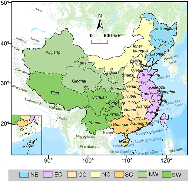
Figure 1. Study area spatial distribution map.
2.2. Data source
The daily maximum 8-h O3 concentration (MDA8) reanalysis dataset of 10 × 10 km from January 1, 2013, to December 1, 2018, is from the tracking air pollution in China (http://tapdata.org/). The dataset is based on a machine learning algorithm and multi-data information fusion inversion. Its comprehensive construction combines ground monitoring data, satellite remote sensing data, high-resolution emission inventory data, air quality model simulation, and other multi-source data, which greatly improves the spatial and temporal accuracy of the data inversion results compared with the previous air quality reanalysis data (15). The daily O3 concentrations in 360 prefecture-level cities in China during the study period were obtained from the China National Environmental Monitoring Center (http://www.cnemc.cn/sssj/). In order to reduce the error in the calculation of the health risk model, we calculated the 90th percentile concentration of the MDA8 O3 concentration from the interannual scale based on the daily MDA8 O3 concentration as the threshold.
The population size (Pop), the proportion of secondary industry to GDP (S_GDP), disposable income per capita (P_GDP), and soot emissions (Dust) for 360 prefecture-level cities in China during the study period were obtained from the China Statistical Yearbook (http://www.stats.gov.cn/tjsj/ndsj/#). The nitrogen oxide (NOx) and volatile organic compound (VOC) emissions were obtained from the China Multiscale Emissions Inventory Model (http://meicmodel.org/). The 1 × 1 km spatial resolution population data were obtained from the World pop dataset (https://www.worldpop.org/).
The daily meteorological data were obtained from the China Meteorological Data Network (http://data.cma.cn/) during the study period. The meteorological data obtained in this study mainly include air temperature (Tem, °C), sea level pressure (Pa, Pa), relative humidity (Hum, %), 2-m mean wind speed (WS, m/s), 1-h precipitation (Pre, mm), and 10-min mean visibility (Vis, m).
2.3. Trend analysis
Trend analysis is usually used for the analysis of temporal dynamics of air pollutants to explore the interannual rate of pollutant changes (16). In this paper, the rate of change of O3 concentrations in China from 2013 to 2018 was analyzed based on the trend analysis method, which is calculated as Equation (1):
Where O3 indicates the O3 concentration of each cell; n indicates the time span, here the time span is 6; and i is the time unit.
2.4. Population exposure risk model
Previous studies have shown that significant heterogeneity in the spatial distribution of air quality concentrations and population density leads to major spatial differences in the exposure risks of populations to air quality (17). In addition, health risks due to exposure to pollutants are usually defined as a function of the multiplication of population density and pollutant concentration (18). Although the exposure risk intensity in the area can be quantified to some extent, it cannot distinguish the severity of the local area relative to the whole. To address this issue, we introduced a model for the relative exposure risk of the population attributable to O3 exposure, as shown in Equation (2), which can evaluate the exposure status in each pixel of the cells (19):
where Ri indicates the risk of population exposure in grid cell i; Pi indicates the number of exposed populations in grid cell i; Ci indicates the O3 concentration in grid cell i, and n indicates the total number of grid cells in the study area. To better reflect the spatial difference of relative population exposure risk, we categorized the population exposure risk as extremely low risk, low risk, lower risk, higher risk, high risk, and extremely high risk by using the reclassification method in ArcGIS10.8 software. The corresponding exposure risk values are Ri = 0, 0 < Ri ≤ 1, 1 < Ri ≤ 2, 2 < Ri ≤ 3, 3 < Ri≤ 5 and Ri> 5, respectively. A higher value of R indicates a higher exposure risk.
2.5. Health risk model
In this study, a standard damage function was applied to estimate the population of premature deaths from respiratory diseases due to O3 exposure. The specific equations are shown in Equations (3) and (4), and the relationships shown in the following equations have been extensively applied in previous studies (14, 20, 21).
where RR is the relative risk; (RR−1)/RR is the attributable fraction; xi is the O3 concentration in a city i or grid i; x0 is the threshold concentration; β is the exposure-response coefficient, which represents the additional health risk associated with an increase in unit O3 concentration (22, 23); ΔM is the number of premature deaths of respiratory diseases attributable to exposure to the O3 environment; y0 is the baseline mortality rate of respiratory diseases, and pop is the number of the exposed population. In this study, the mortality rate of respiratory diseases was obtained from the National Bureau of Statistics, where the crude mortality rate of respiratory diseases y0 (1/100,000) in urban China from 2013 to 2018 was, 76.61, 74.17, 73.36, 69.03, 67.20 and 68.02, respectively. β values in this study were obtained from Shang et al. (24), per 10 μg/m3 with a value of 0.48% (95% CL: 0.38%, 0.58%). Song et al. (25) concluded that the exposure-response coefficients obtained from a meta-analysis by Shang et al. (24) based on a 33–time series and case-crossover study conducted could to some extent reflect the health risks attributed to air pollution in China. Meanwhile, which has widely been used in several past studies for China (26, 27).
2.6. Multi-scale geographically weighted regression
Compared with the classical geographically weighted regression model (GWR), the MGWR model was a flexible regression model (28). Each regression coefficient was obtained based on local regression, and the bandwidth is specific. In addition, the GWR model uses weighted least squares in the fitting operation, while the MGWR model was equivalent to a generalized additive model (GAM), which could perform regression analysis on spatial variables with linear or non-linear relationships, and was also an effective tool for dealing with various complex non-linear relationships of spatial variables (29). Assuming that there are n observations, for observation i ∈ {1,2,3,…, n} at location (Ui, Vi), the MGWR were calculated as follows (30):
where yi is the response variable O3 concentration, β0(Ui, Vi) is the intercept, Xij is the jth predictor variable i, βbwj(Ui, Vi) is the jth coefficient, bwj in βbwj indicates the bandwidth used for calibration of the jth conditional relationship, εi is the error term. In addition, the spatial kernel function type selected during the model operation is bisquare, the bandwidth search type is golden, and the model parameter initialization type takes GWR estimation as the initial estimation model.
2.7. Research framework
This study used the trend analysis method, spatial autocorrelation model, population exposure risk model, exposure-response function, and MGWR model to analyze the spatial-temporal pattern, exposure risk, health risk, and driving factors of O3 concentration in China from 2013 to 2018. Firstly, we use the trend analysis method and spatial autocorrelation model to explore the changing trend and spatial-temporal distribution of O3 concentration in China. Secondly, we selected the population exposure risk model and exposure-response function to investigate the population exposure risk and health risk attributed to O3 pollution, and discussed their temporal and spatial correlation characteristics. Finally, we use the MGWR model to reveal the dominant factors of spatial distribution difference of O3 concentration in China. Additionally, in this study we used O3 concentration reanalysis data at 10 × 10 km resolution and population raster data at 1 × 1 km resolution to investigate the exposure risks and health risks attributed to O3 pollution. To spatially match the 10 × 10 km O3 concentration reanalysis data, we used the aggregation module of ArcGIS10.6 software to quantitatively change the spatial resolution of the 1 km × 1 km population data. During the aggregation calculation, the output image element cell size was set to 10 × 10 km, i.e., 0.01° × 0.01°, and the nearest neighbor assignment method was selected for the aggregation technique. Figure 2 shows the research framework of this paper.
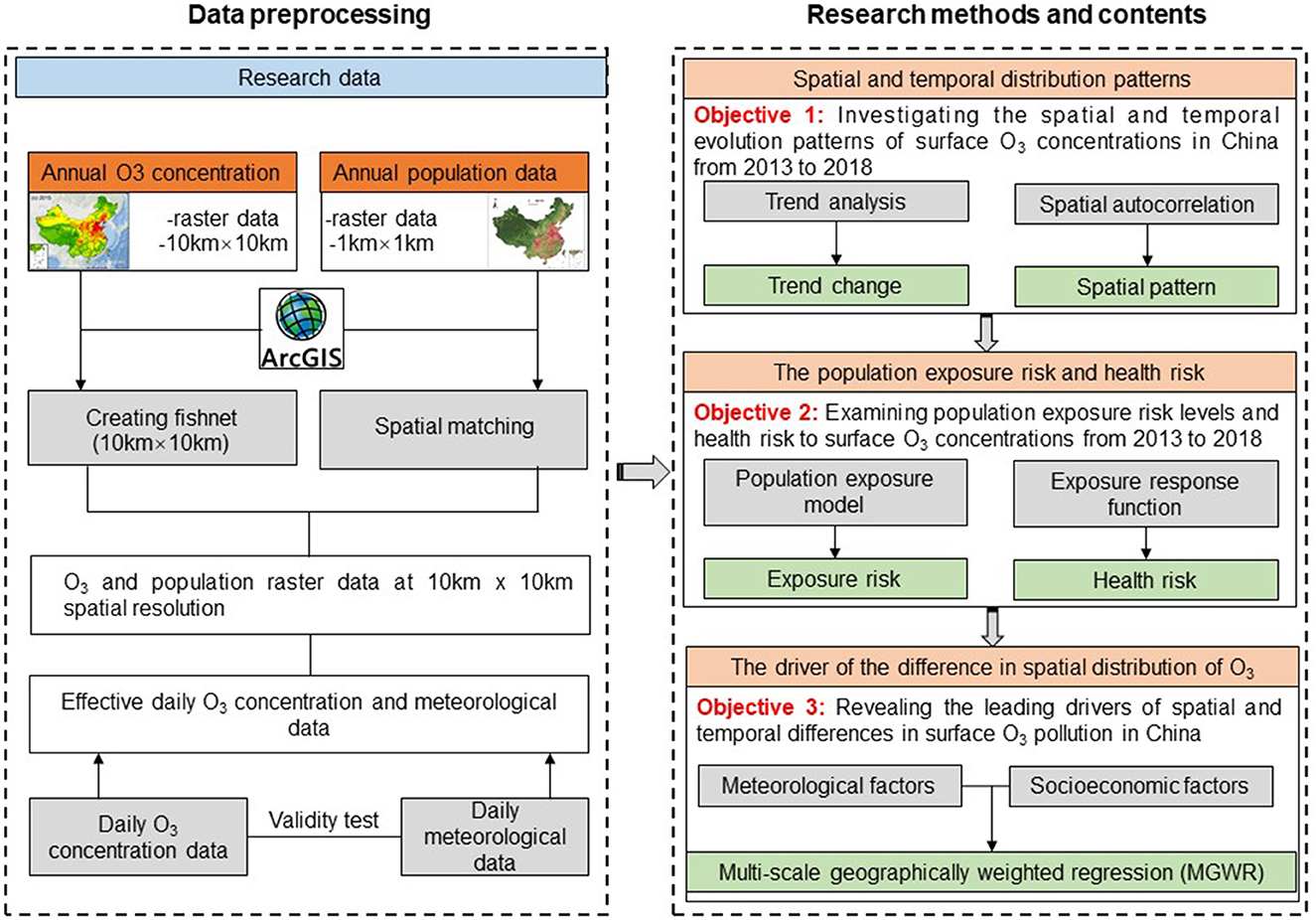
Figure 2. Research framework.
3. Results
3.1. Spatial and temporal distribution patterns
Figure 3 shows the temporal and spatial distribution and changing trend of the annual average concentration of MDA8 (AMDA8, O3) from 2013 to 2017 in China. From 2013 to 2018, the annual average O3 concentrations in China were 110.75, 108.21, 111.13, 115.57, 120.49, and 115.95 μg/m3, respectively, and changed at a rate of 1.84 μg/m3/yr increase (Figure 3H). From a spatial and temporal perspective, the highest annual average O3 concentrations were found in central China in 2013, 2015, and 2016, with annual average O3 concentrations of 121.87, 118.84, and 122.78 μg/m3, respectively. The highest annual average O3 concentrations in 2014, 2017, and 2018 were all found in East China, with annual average O3 concentrations of 116.98, 135.03, and 137.91 μg/m3, respectively. In comparison, the lowest O3 concentration in 2013 occurred in the Northeast region (98.33 μg/m3), the lowest O3 concentrations from 2014 to 2017 occurred in the Southwest region of China (90.86, 94.43, 99.20, and 104.27 μg/m3), and the lowest O3 concentration in 2018 occurred in the Northwest region (103.44 μg/m3) (Figures 3A–G). Since 2013, 89.62% of China's territory has experienced a significant increase in annual average O3 concentrations, with 2.73% of the regions experiencing an average rate of change in annual average O3 concentrations exceeding 5.00 μg/m3/yr. However, the rate of variation of O3 concentration varies from region to region has strong spatial variability. The rate of change of O3 concentration in the Central Plains urban agglomeration is the most variable in terms of the country, with its O3 concentration change rate exceeding 4.0 μg/m3/yr. In contrast, the rate of change of O3 concentration in the Chengdu-Chongqing urban agglomeration (−0.3 ± 1.0 μg/m3/yr), Southwest China (−0.5 ± 1.1 μg/m3/yr) and South China (−1.0 ± 1.4 μg/m3/yr) decreases significantly (Figure 3G).
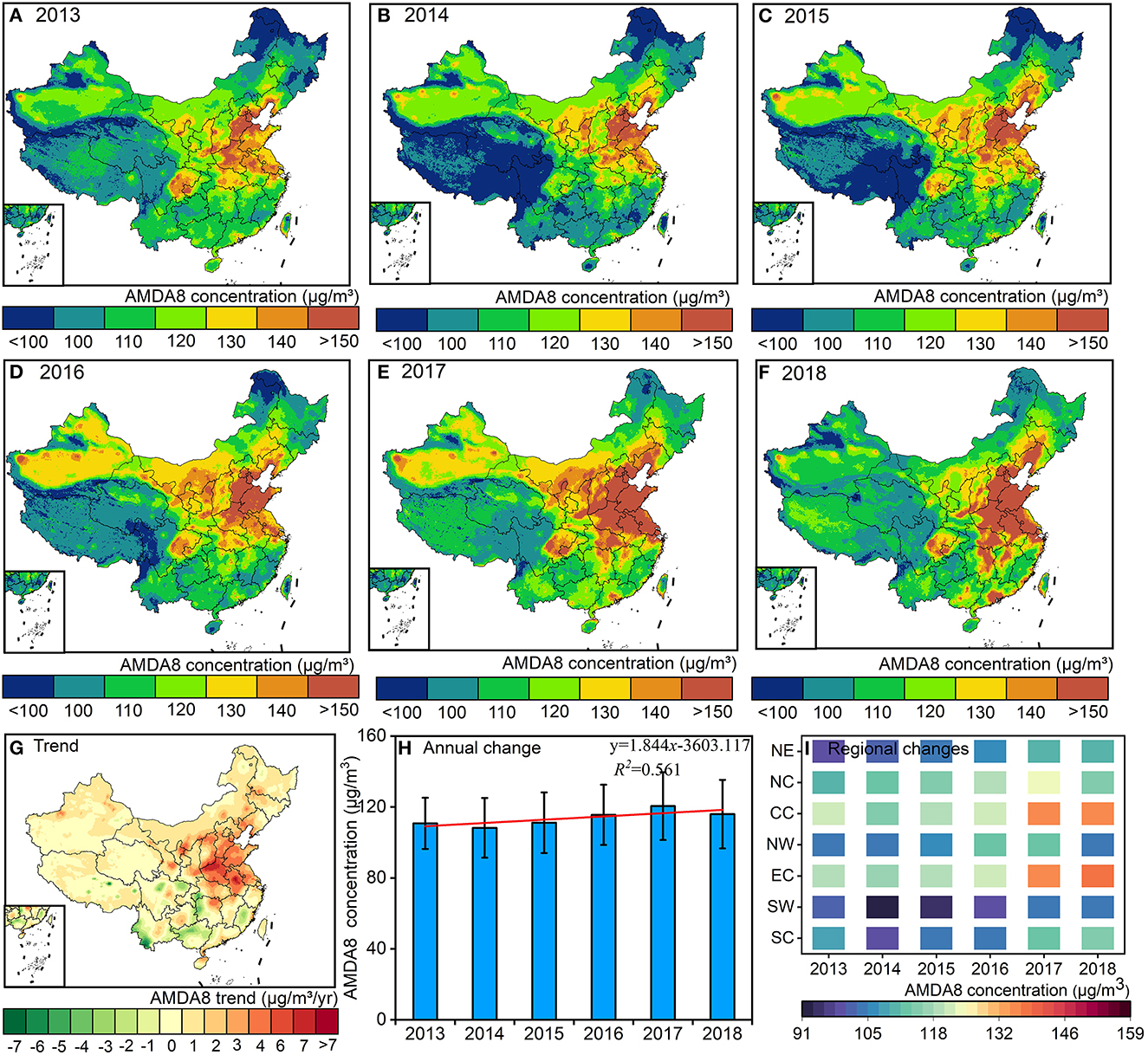
Figure 3. The spatial distribution and trend of O3 concentration from 2013 to 2018. Where, (A–F) represents the spatial distribution of O3 concentration; (G) represents the trend change of O3 concentration; (H) represents the annual average O3 concentration variation; (I) shows the annual average O3 concentration change in different regions of China.
Figure 4 represents the spatial clustering characteristics of the rate of variation of O3 concentration at county-level units in China from 2013 to 2018. The results show that the global Moran's I index is significant at the 1% level, indicating a consistent and enhanced positive spatial autocorrelation in the rate of variation of O3 concentration (Figure 4A). The results of the hot spot analysis show that there is a significant hot spot (HH) region for O3 concentration growth rate, which is mainly contiguous and focused in Shaanxi, Shanxi, central Inner Mongolia, Beijing–Tianjin–Hebei (BTH), southwest Liaoning, central Henan, eastern Hubei, Anhui, Jiangsu, and Shandong in China, which are the regions with the strongest O3 growth rate in China. In addition, we found a significant cold spot area (LL) covering a large part of China (about 90% of the territory). These regions are mainly located in northeastern, southern, southwestern, eastern, and northwestern China, where the growth rate of O3 concentration is relatively low and even decreasing regions are observed (Figures 4B, C). The standard deviation ellipsometric analysis evaluated the overall variations in the spatial pattern of O3 concentration growth rate from 2013 to 2018 in China (Figure 4D). It can be found that the regions with significantly increased O3 concentration growth rates are mainly concentrated in BTH, Shanxi, Shandong, Jiangsu, Jiangxi, Anhui, Hubei, Henan, and Shaanxi in China. This result also indicates that the above-mentioned regions are the primary contributors of O3 during the whole study period in China. Meanwhile, the center of the median growth rate of O3 concentration is located north of the standard deviation ellipse arithmetic center, indicating that the growth rate of surface O3 concentration is greater in northern China than in southern China.
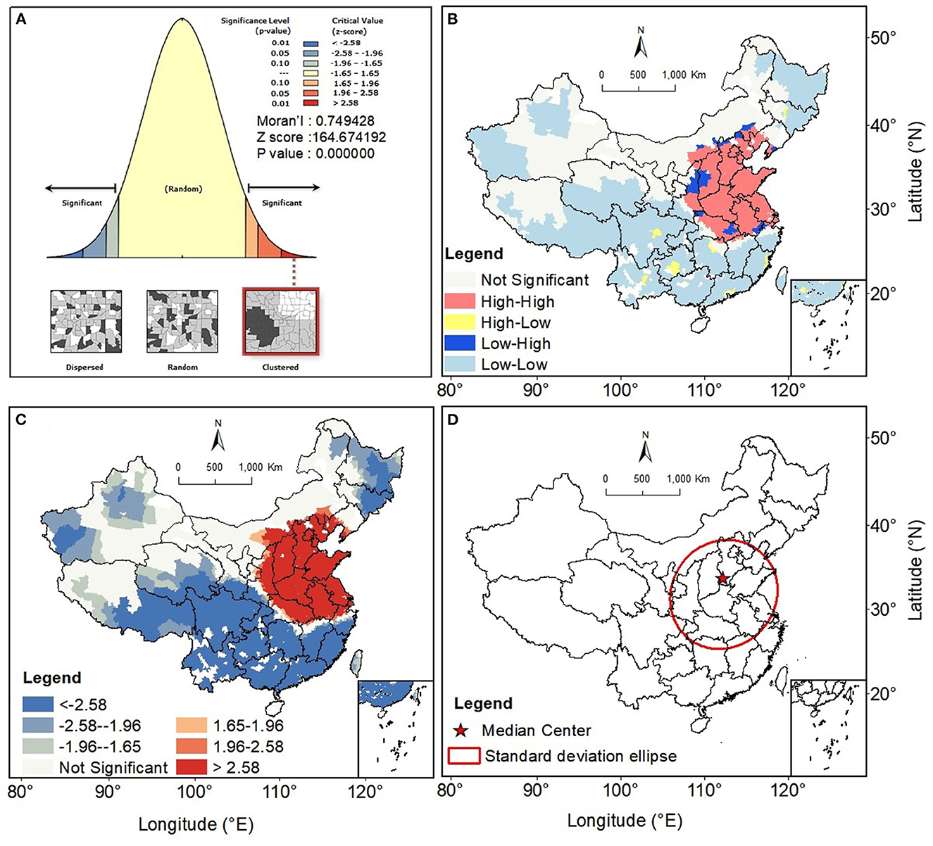
Figure 4. Spatial clustering characteristics of the rate of change of O3 concentration in county-level units in China, 2013–2018. (A) Global spatial autocorrelation test results; (B) Spatial distribution of the spatial clustering of O3 concentration variation rates; (C) Spatial distribution of cold and hot spots for the rate of change of O3 concentration, in the cold and hot spot analysis we used Getis Ord Gi* analysis to calculate Z scores, where |Zscores| > 1.65 corresponds to p < 0.10, |Zscores| > 1.96 corresponds to p < 0.05, |Zscores| > 2.58 corresponds to p < 0.01. Z scores are negative indicating a cold spot, and a positive Z score indicates a hot spot; (D) Spatial distribution of the standard ellipse of the rate of variation of surface O3 concentration and the center of change in China from 2013 to 2018.
3.2. The population exposure risk and health risk
Overall, the total population exposed to O3 > 160 μg/m3 increased from 1.2% in 2013 to 28.9% in 2018, compared to a decrease in the population exposed to O3 < 160 μg/m3 from 7.2% in 2013 to 3.6% in 2018 (Figure 5). Figures 6, 7 represents the spatial pattern of exposure risk levels attributed to O3 pollution in 2013, 2015, and 2018. We found that most regions have remained at low (52.89–55.73%) or extremely low (19.48–20.48%) O3 exposure risk levels over three time periods in China. From a temporal perspective, only 4.83% of the territory of the country was at high exposure to O3 pollution in 2013, and this percentage increased to 6.45 and 7.19% in 2015 and 2018, respectively. Similarly, the area of the territory exposed to extremely high risk also exhibits a marked increasing trend, from 7.61% in 2013 to 9.62% in 2015 and further to 11.35% in 2018 (Figures 7A–C). Spatially, the distribution patterns of O3 exposure risk levels were similar for the three time periods of 2013, 2015, and 2018 in China. With the rapid increase of O3 concentration in the North China Plain, the high exposure risk level regions of BTH and YRD have been continuous, which constitute a high O3 exposure risk level aggregation area including the Bohai Rim, YRD, Pearl River Delta (PRD), Shanxi and Guanzhong Plain urban clusters. Spatially, the distribution patterns of O3 exposure risk levels were similar for the three time periods of 2013, 2015, and 2018 in China. In contrast, the extremely low risk and lower risk areas of O3 pollution are widely distributed in China, which is mainly located in most regions of northwest, southwest, and northeast in China (Figures 7D–F).
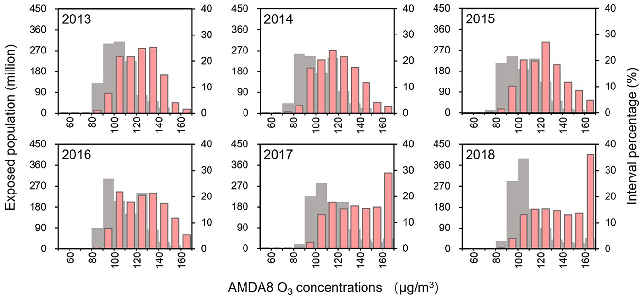
Figure 5. Probability distribution of the total population exposed to different O3 concentrations from 2013 to 2018. The red and gray bars indicate the total population and the proportion of the population exposed to different O3 concentrations, respectively.
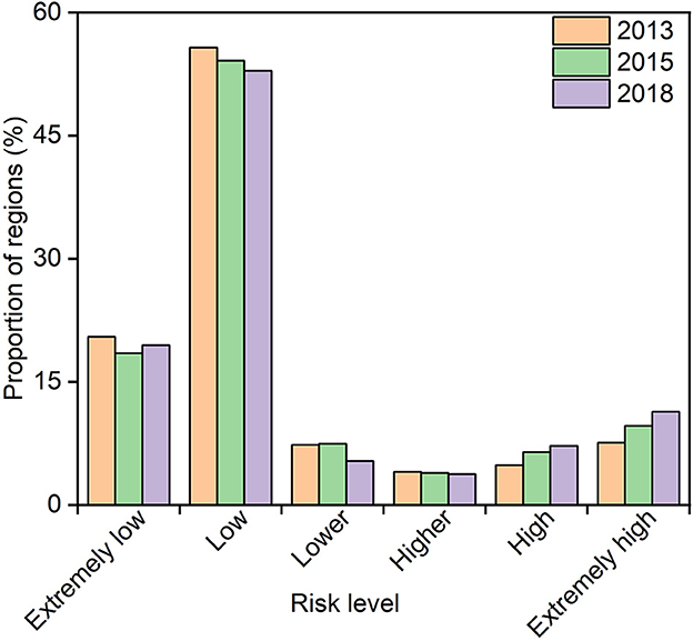
Figure 6. Proportion of regions with different O3 exposure risk levels to the total land area (%).
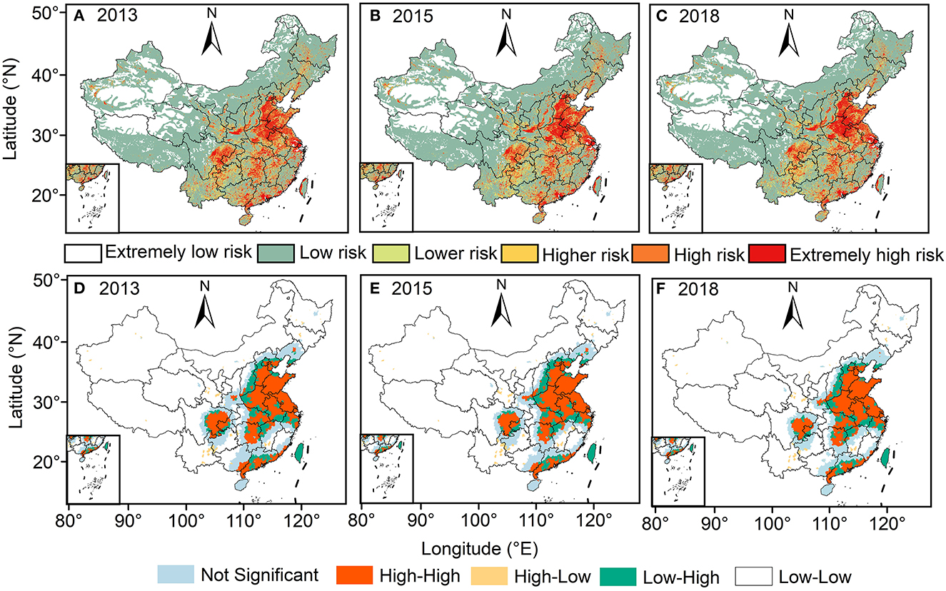
Figure 7. Spatial distribution pattern of population exposure risk levels attributed to O3 pollution from 2013 to 2018. (A–C) Indicates the spatial distribution of population exposure risk levels in 2013, 2015, and 2018, respectively; (D–F) Indicates the spatial clustering of population exposure risk levels in 2013, 2015, and 2018, respectively.
Figure 8 indicates the spatial and temporal distribution of premature deaths from respiratory diseases attributable to O3 exposure from 2013 to 2018. Overall, there was an average of over 24,000 premature deaths from respiratory diseases due to O3 exposure per year in China from 2013 to 2018, and the growth rate fluctuated at 1,178 cases per year (p < 0.05). Specifically, the number of premature deaths attributable to O3 exposure increased from 236,200 in 2013 to 272,300 in 2018, an increase of 36,100 cases compared to 2013. Spatially, the regions with <500 cases of premature death due to O3 exposure are mainly located in Tibet, Qinghai, east of Xinjiang, west of Sichuan, west of Inner Mongolia, Liaoning, and Heilongjiang; the regions with more than 500 cases are mainly located in the region east of Hu line, mainly including most of eastern China and western Xinjiang, central Inner Mongolia, southern Gansu, most of southern China, most of northern China, and Liaoning in northeast China. The regions with more than 1,000 cases are mainly located in BTH, Sichuan–Chongqing region, Fenwei Plain, East China Plain, Jianghan Plain, Yangtze River Delta, and Pearl River Delta region. Meanwhile, the regions with more than 1,000 cases of premature death due to O3 exposur e are further expanding over time.
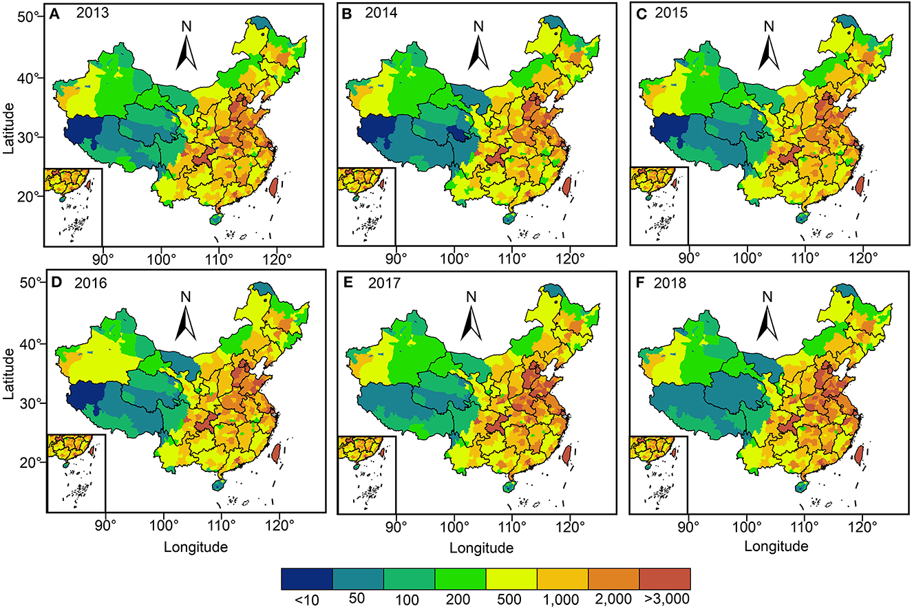
Figure 8. Spatial distribution of premature deaths attributable to O3 exposure in China, 2013 to 2018. (A–F) indicates the spatial distribution of premature death population attributable to O3 exposure at the prefecture-level city scale from 2013 to 2018 in China, respectively.
3.3. The driver of the difference in the spatial distribution of O3
Multicollinearity refers to the distortion of model estimates due to significant correlations between the independent variables in the linear modeling regression process. Therefore, before conducting model regression analysis, to test whether there is multicollinearity between each explanatory variable, we use variance inflation factor (VIF) to test the multicollinearity problem between each explanatory variable, and previous studies have shown that when VIF ≥ 10, it indicates that there is a serious multicollinearity problem between the dependent variable and the independent variable. multicollinearity problem, which should be removed from the actual model operation. The collinearity test in this study was performed in SPSS 25.0 software and the results of the analysis showed that the range of VIF values for all explanatory variables was 1.000–9.765, which indicates that there was no cointegration between the dependent and independent variables. Table 1 indicates the diagnostic information of the MGWR model for the socioeconomic and meteorological factors. In terms of the number of valid parameters, the goodness–of–fit R2 for the responses of socioeconomic and meteorological factors to O3 concentrations are 0.861 and 0.799, respectively, and the residual sum of squares (RSS) is 136.297 and 136.51 μg/m3, respectively, with the absolute values of the deficit information criterion (AIC) and the log-likelihood value (Log-likelihood) < 5,000. These regression results indicate that MGWR uses fewer parameters to obtain regression results that are closer to the true values and can be fully used to assess the relationship between O3 pollution and socioeconomic and meteorological factors.
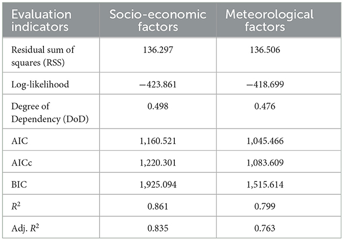
Table 1. Diagnostic information of MGWR model.
Figure 9 indicates the spatial distribution of regression coefficients of socio-economic factors. The high values (>0.27) of regression coefficients for the total population are mainly located in North and East China, where the total population is significantly and positively correlated with its corresponding O3 concentration. The influence of the share of secondary industry on surface O3 in East and North China is significantly higher than that in other regions, and its regression coefficient exceeds 0.08. We also find that over 80% of the regional disposable income per capita is positively correlated with O3, with regression coefficients ranging from 0.07 to 0.36. In contrast, Guangdong, Shandong, and Northeast provinces show a significant negative correlation between disposable income per capita and O3, with regression coefficients, were below −0.02. The industrial dust emissions in Sichuan and Chongqing are significantly (p < 0.001) positively correlated with the corresponding O3 concentration with a regression coefficient > 0.52, while industrial dust emissions in cities located in East China are significantly (p < 0.01) negatively correlated with the corresponding O3 concentration with a regression coefficient ranging from −0.53 to −0.25, where O3 concentrations in cities located in eastern Jiangsu and Anhui provinces are more affected by the negative correlation of industrial dust emissions. The NOx emissions were significantly and positively correlated with O3 concentrations in Central China, East China, South China, Sichuan and Chongqing, and parts of Southwest and Northwest China (p < 0.05), with regression coefficients ranging from 0.60 to 1.26. There was a significant (p < 0.01) negative correlation between VOCs emissions and O3 concentrations in Hubei, Jiangxi, Zhejiang, Anhui, Jiangsu, Shanghai, Guangdong, Fujian, and Guangxi cities with regression coefficients ranging from −0.53 to −0.35.
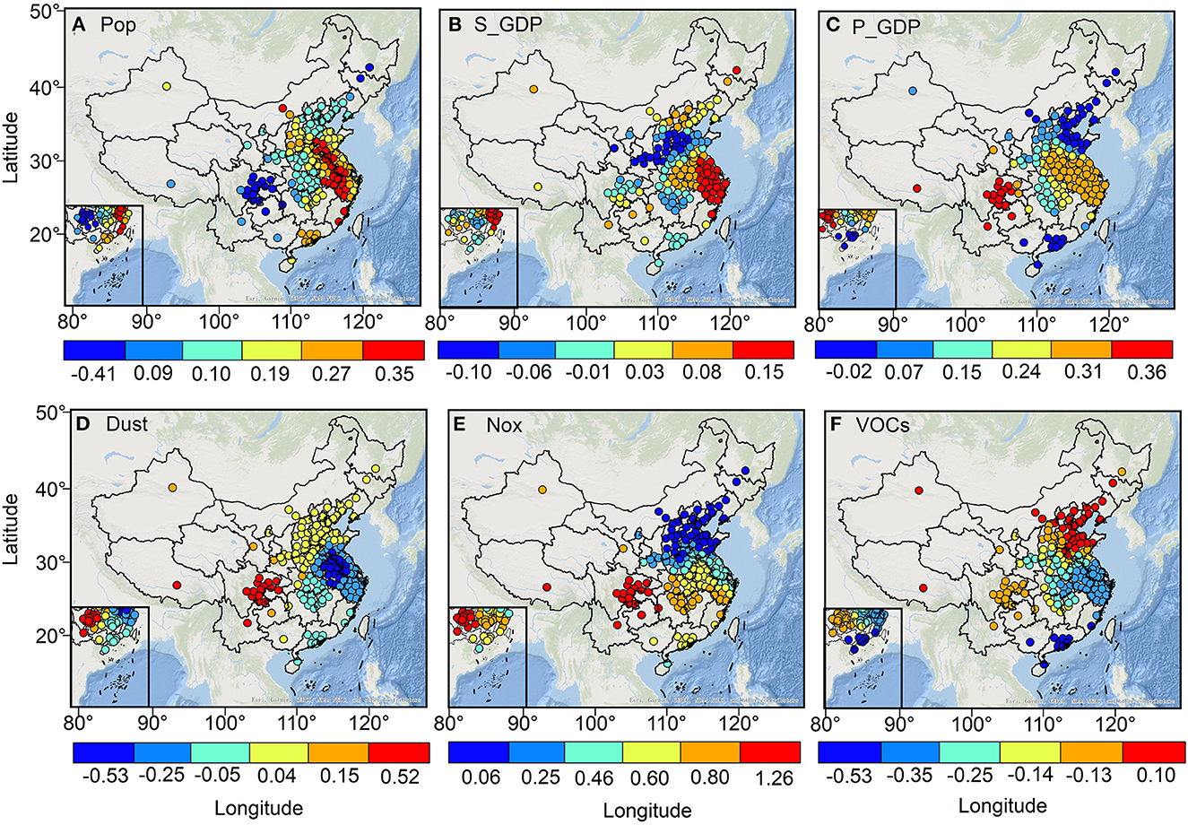
Figure 9. The spatial distribution of regression coefficients for the major socioeconomic factors of Pop (A), S_GDP (B), P_GDP (C), Dust (D), NOx (E), and VOCs (F).
Figure 10 shows the spatial differences in the effects of various meteorological factors on O3 concentration. It can be found that the temperature of cities in North, East, and Northeast China showed a significant (p < 0.05) positive correlation with O3 concentration, with regression coefficients ranging from 0.23 to 0.49. The relative humidity was negatively correlated with O3 concentration in all cities during the study period. Among them, cities in Heilongjiang, Jilin, Liaoning, Beijing, Tianjin, north-central Hebei, northwestern Shanxi, western Inner Mongolia, and northwestern Ningxia and northern Shaanxi showed a weak negative correlation between relative humidity and O3 concentration with a non-significant (p > 0.05) regression coefficient of < −0.07. In contrast, cities in southern Zhejiang, southern Anhui, Jiangxi, central Hubei, Hunan, Chongqing, Guizhou, Yunnan, and cities in Fujian, Guangdong, and Guangxi regions showed a significant (p < 0.01) strong negative correlation between relative humidity (Hum) and its corresponding O3 concentration with regression coefficients ranging from −0.18 to −0.15. Wind speed (WS) showed a significant (p < 0.05) negative correlation with O3 concentrations in Heilongjiang, Jilin, Liaoning, Guangxi, southern Henan, Hubei, eastern Shandong, Jiangsu, Shanghai, Zhejiang, Sichuan and Chongqing regions, and northern Shanxi, with regression coefficients ranging from −0.02 to −0.06. It is particularly noteworthy that cities in BTH, southwestern Shanxi, northern Henan, central Shaanxi, Ningxia, southern Gansu, western Shandong, and Anhui have a significant positive correlation between their wind speed and O3 concentration with regression coefficients >0.45. For air pressure, cities located in northern China showed a significant (p < 0.05) negative correlation between air pressure (Pa) and O3 concentration, with regression coefficients ranging from −3.6 × 10⁻³ to −1.3 × 10⁻³. Precipitation showed a significant (p < 0.05) positive correlation with O3 concentration in Heilongjiang, Jilin, South China, Guangxi, and Guangdong, with regression coefficients ranging from 3.93 to 19.21, while other regions showed negative correlations. Visibility was positively correlated with O3 concentration in all cities.
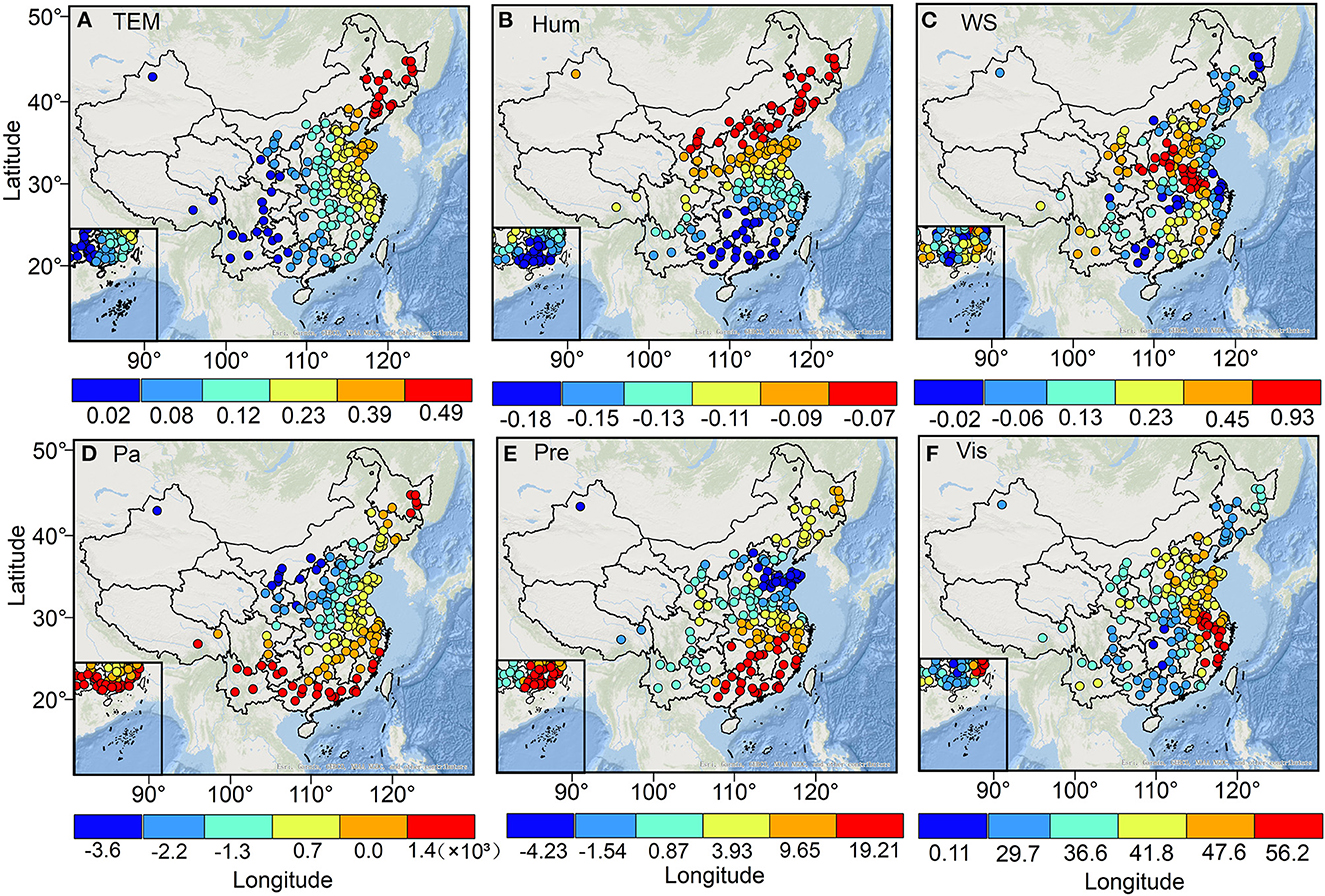
Figure 10. The spatial distribution of regression coefficients for the major meteorological factors of TEM (A), Hum (B), WS (C), Pa (D), Pre (E), and Vis (F).
4. Discussion
4.1. Spatial distribution difference of O3 concentration
The results of the spatial and temporal pattern analysis of O3 concentrations show that East, Central, and North China are the regions with the highest growth of O3 concentrations in China from 2013 to 2018, which is mainly attributed to the huge amount of anthropogenic emissions. The areas of East, Central, and North China are one of the most densely populated and industrially developed regions in China, and the massive industrial activities, transportation, and human activities result in the emission of large amounts of O3 precursors. In contrast, Southwest and South China are the regions with the largest decreases in O3 concentrations in China. Previous studies have found that Southwest and Northwest China are located in high-latitude regions, and their corresponding atmospheric vertical exchange and photochemical reactions are stronger due to the special topography and intense solar radiation compared to inland regions, resulting in higher background values of O3 concentrations in these regions (9, 31). However, the extent of the influence of solar radiation on O3 in southwest and southern China is significantly weaker than the influence of anthropogenic emissions compared to the dramatic increase in O3 concentrations due to strong anthropogenic emissions in East, Central, and North China (32).
4.2. Spatial heterogeneity of O3 concentration drivers
There are strong spatial variations in the influence of different drivers on O3. Relative to lower population density regions, a larger population size implies more energy consumption and pollution emissions, meanwhile, it also further compresses the green area of cities, leading to a significant reduction in the ability of cities to mitigate air pollution, which better explains why the positive correlation between population size and O3 concentration is significantly higher in densely populated northern and eastern China than in other regions (21, 33). Previous studies have shown that industrial emissions are the predominant source of air pollution (34). Our study found that the share of secondary industry in GDP had a significant positive correlation with O3 concentration, especially in central China, and eastern China, where industrial production is dominant, and the contribution of urban industrial production to O3 concentration is stronger than in other regions. At the urban scale, the formation of O3 concentrations depends on the VOCs–NOx ratio (35). In general, the higher the NOx emissions in cities, the lower the VOCs–NOx ratio. For example, the formation of O3 in some cities located in Central and Northern China is often limited by VOCs (36, 37). In these cities, the reduction of VOCs emissions decreases the formation of O3, but the reduction of NOx emissions increases the formation of O3. This chemical reaction tends to depend on the amount of VOCs and NOx emissions; the larger the emissions the more intense their reaction and the larger the O3 emissions generated (38). In addition, industrial dust emissions indirectly affect solar radiation intensity by affecting atmospheric visibility, which further contributes to the O3 photochemical reaction rate (39).
Temperature is an important ambient condition for photochemical reactions, and higher temperatures can promote the rapid production of O3 concentration, therefore, temperature and O3 concentration are mostly positively correlated, especially in cities in Northern, Eastern, and Northeastern China where the solar temperature is higher in the warm season (40). The wind speed has a diffusion and transport effect on pollutants in the atmosphere. For example, O3 concentrations in cities in Northeast, South, Central, and East China, and Sichuan and Chongqing regions showed a significant (p < 0.05) negative correlation with wind speed. However, our results found a significant positive correlation between O3 concentration and wind speed in most cities located in the North China Plain. Li et al. (41) attributed the significant positive correlation between O3 concentration and wind speed in the North China Plain region to the influence of warm-season burning winds, especially from June to August each year, when the burning winds blow from the mountains to the northern and western parts of the North China Plain, bringing dry the hot air further leads to a higher temperature in the region, which accelerates the photochemical reaction of O3 production to some extent. Relative humidity has a negative correlation with O3 concentration. Previous studies have shown that water vapor can not only absorb and release energy through changes in the aqueous phase but also undergo internal reactions, especially when controlling for other influencing factors, higher relative humidity leads to higher water vapor saturation, resulting in easy removal of O3 and its precursors and lower O3 concentrations (42). In addition, water vapor can reduce solar ultraviolet radiation through extinction mechanisms, thus affecting photochemical reactions and O3 concentrations (43).
4.3. The O3 control policy implications
In summary, O3 pollution in China is gradually increasing, and more and more of China's population is exposed to high O3 concentration pollution. Scientific and effective reduction of O3 concentration exposure levels in China is crucial to reduce population exposure risks (44). Under these circumstances, this study proposes policy recommendations on how to reduce O3 concentrations in Chinese cities from the perspective of the drivers affecting the spatial distribution of O3 and epidemiology. For O3 pollution areas dominated by O3 precursors (e.g., NOx, VOCs, and CO), the authorities can ensure that their emissions comply with government regulations by optimizing the industrial structure and reducing the emissions of O3 precursors. Meanwhile, the governmental department should focus on the synergistic management of PM2.5 and O3 compound pollution. Research shows that NOx is not only an important precursor for O3 generation but also an important precursor for PM2.5 (45). Therefore, strengthening the NOx deep regulation and emission reduction is a key step to promote synergistic control. Furthermore, the O3 abatement measures in the future should pay attention to different seasonal O3 control measures and strengthen regional cooperation for O3 pollution prevention.
For O3 pollution regions dominated by meteorological factors, the department should forecast the variation of O3 concentration due to the change of meteorological factors promptly, meanwhile develop a detailed O3 pollution early warning program to reduce the risk of public exposure and explore a sustainable development path for O3 pollution management in China. From an epidemiological perspective, to protect public health and improve the status of O3 pollution, it is crucial to establish studies of health effects attributed to O3 exposure from a national perspective. In addition, it is important for relevant government departments to establish a mechanism to revise the National Ambient Air Quality Standards (NAAQS) for regulatory assessment and health risk prediction of future O3 air quality standards in China (46).
4.4. Research limitations and future prospects
Surface O3 distribution has strong spatial and temporal heterogeneity, and there are significant differences in O3 concentrations with time scales. This study only focused on the interannual spatial variability characteristics of O3 concentrations, neglecting the seasonal variability of O3 concentration changes. Furthermore, due to the lack of basic research data and inadequate research methods, this study only focused on the number of premature respiratory deaths attributed to O3 pollution in the assessment of health risks attributed to O3 pollution, neglecting the all-cause premature death group. Additionally, using the same exposure risk coefficient (β) may lead to spatial errors in the estimated health risks due to significant spatial differences in O3 exposure levels. For example, Wang et al. (21) estimated the population of premature deaths from respiratory diseases caused by O3 pollution between 2013 and 2017 in China using the method of Turner et al. (47), and their results found an average of 186,000 deaths from respiratory diseases due to O3 pollution during the study period. This is slightly lower compared to our findings. A primary reason for this is that our study and Wang et al. (21) used different exposure response coefficients and critical thresholds. In addition, the interpolation of O3 concentrations at large scales of pollution can also cause large errors in the assessment results. Therefore, in the future, we hope to conduct a detailed and comprehensive analysis of seasonal differences in O3 pollution and all-cause health risks in China by utilizing more detailed surface O3 monitoring data and meta-analysis methods. To provide a scientific basis for the improvement of O3 pollution in China.
5. Conclusions
In this study, we quantitatively investigated the spatial and temporal patterns, trends, population exposure risks, health risks, and drivers of surface ozone in China from 2013 to 2018. We observed the annual average O3 concentration of China increased significantly at a rate of change of 1.84 μg/m3/yr from 2013 to 2018 (p < 0.05, R2 = 0.561). The significant increase was mainly distributed in East China, Central China, and North China. Meanwhile, the growth rate of O3 concentration has a consistent and enhanced positive spatial autocorrelation (p < 0.05), and there are significant hot and cold spots areas. During the research period, there was an average of over 24,000 premature deaths from respiratory diseases attributed to O3 exposure in China from 2013 to 2018, and the growth rate fluctuated at 1,178 per year (p < 0.05). Spatially, there was a consistency in the spatial distribution of exposure risk and health risk of populations exposed to O3. The results of the multi-scale geographically weighted regression model reveal spatial differences in the effect of various factors on O3 concentration. The impact of the total population, disposable income, the share of secondary industry in GDP, and NOx emissions factors in eastern and northern regions are significantly greater than impacts in central and western regions. Meanwhile, we found that the effect of temperature on O3 concentration in some cities in the north, east, and northeast is significantly higher than that in other regions, and relative humidity has a significant (p < 0.01) strong negative correlation with O3 concentration in east, central, southwest and south China.
Data availability statement
The datasets presented in this study can be found in online repositories. The names of the repository/repositories and accession number(s) can be found in the article/supplementary material.
Author contributions
CH conceived the idea of the study and designed research, wrote the paper, discussed the results, and revised the manuscript. LZ conceived the idea of the study and design research, discussed the results, and revised the manuscript. XG involved in funding acquisition, resources, supervision, and analyzed the data. BL and JL discussed the results and revised the manuscript. QW analyzed the data, discussed the results, and revised the manuscript. All authors contributed to the article and approved the submitted version.
Funding
This work was supported by the Natural Science Foundation of Hubei Province (2020CFB478).
Conflict of interest
The authors declare that the research was conducted in the absence of any commercial or financial relationships that could be construed as a potential conflict of interest.
Publisher's note
All claims expressed in this article are solely those of the authors and do not necessarily represent those of their affiliated organizations, or those of the publisher, the editors and the reviewers. Any product that may be evaluated in this article, or claim that may be made by its manufacturer, is not guaranteed or endorsed by the publisher.
References
1. Hu BF, Shao S, Ni H, Fu ZY, Huang MX, Chen QX, et al. Assessment of potentially toxic element pollution in soils and related health risks in 271 cities across China. Environ Pollut. (2021) 270:116196. doi: 10.1016/j.envpol.2020.116196
2. Zhan CC, Xie M, Liu JN, Wang TJ, Xu M, Chen B, et al. Surface ozone in the Yangtze River delta, China: a synthesis of basic features, meteorological driving factors, and health impacts. J Geophys Res Atmos. (2021) 126:e2020JD033600. doi: 10.1029/2020JD033600
3. Gao D, Xie M, Liu J, Wang TJ, Ma CQ, Bai HK, et al. Ozone variability induced by synoptic weather patterns in warm seasons of 2014-2018 over the Yangtze River Delta region, China. Atmos Chem Phys. (2021) 21:5847–64. doi: 10.5194/acp-21-5847-2021
4. Zhan CC, Xie M. Land-surface forcing and anthropogenic heat modulate ozone by meteorology: a perspective from the Yangtze River Delta region. Atmos Chem Phys Discussions. 22:1351–71. (2021). doi: 10.5194/acp-2021-619
5. Maji KJ, Ye WF, Arora M, Nagendra SMS. Ozone pollution in Chinese cities: assessment of seasonal variation, health effects and economic burden. Environ Pollut. (2019) 247:792–801. doi: 10.1016/j.envpol.2019.01.049
6. Wu RR, Xie SD. Spatial distribution of ozone formation in China derived from emissions of speciated volatile organic compounds. Environ Sci Technol. (2017) 51:2574–83. doi: 10.1021/acs.est.6b03634
7. Anenberg SC, Horowitz LW, Tong DQ, West JJ. An estimate of the global burden of anthropogenic ozone and fine particulate matter on premature human mortality using atmospheric modeling. Environ Health Perspect. (2010) 118:1189–95. doi: 10.1289/ehp.0901220
8. Ran L, Lin WL, Deji YZ, La B, Tsering PM, Xu XB, et al. Surface gas pollutants in Lhasa, a highland city of Tibet-current levels and pollution implications. Atmos Chem Phys. (2014) 14:10721–30. doi: 10.5194/acp-14-10721-2014
9. Yin XF, Kang SC, de Foy B, Cong ZY, Luo JL, Zhang L, et al. Surface ozone at Nam Co in the inland Tibetan Plateau: Variation, synthesis comparison and regional representativeness. Atmos Chem Phys. (2017) 17:11293–311. doi: 10.5194/acp-17-11293-2017
10. Ren YF, Fang CL, Li GD. Spatiotemporal characteristics and influential factors of eco-efficiency in Chinese prefecture-level cities: a spatial panel econometric analysis. J Clean Prod. (2020) 260:120787. doi: 10.1016/j.jclepro.2020.120787
11. Gong X, Hong S, Jaffe DA. Ozone in China: spatial distribution and leading meteorological factors controlling O3 in 16 Chinese cities. Aerosol Air Qual Res. (2018) 18:2287–300. doi: 10.4209/aaqr.2017.10.0368
12. Cao YF, Qiao X, Hopke PK, Ying Q, Zhang YY, Zeng YY, et al. Ozone pollution in the west China rain zone and its adjacent regions, Southwestern China: concentrations, ecological risk, and Sources. Chemosphere. (2020) 256:127008. doi: 10.1016/j.chemosphere.2020.127008
13. Maji KJ, Ye WF, Arora M, Nagendra SMS. PM2.5-related health and economic loss assessment for 338 Chinese cities. Environ Int. (2018) 121:392–403. doi: 10.1016/j.envint.2018.09.024
14. Lu X, Zhang L, Wang XL, Gao M, Li K, Zhang YZ, et al. Rapid increases in warm-season surface ozone and resulting health impact in China since 2013. Environ Sci Technol Lett. (2020) 7:240–7. doi: 10.1021/acs.estlett.0c00171
15. Geng GN, Xiao QY, Liu SG, Liu XD, Cheng J, Zheng YX, et al. Tracking air pollution in china: near real-time PM2.5 retrievals from multisource data fusion. Environ. Sci. Technol. (2021) 55:12106–15. doi: 10.1021/acs.est.1c01863
16. Shi YS, Matsunaga T, Yamaguchi Y, Li ZQ, Gu XF, Chen XH. Long-term trends and spatial patterns of satellite-retrieved PM2.5 concentrations in South and Southeast Asia from 1999 to 2014. Sci Total Environ. (2018) 615:177–86. doi: 10.1016/j.scitotenv.2017.09.241
17. Chen Y, Ebenstein A, Greenstone M, Li H. Evidence on the impact of sustained exposure to air pollution on life expectancy from China's Huai River policy. Proc Natl Acad Sci USA. (2013) 110:12936–41. doi: 10.1073/pnas.1300018110
18. Peng J, Chen S, Lu HL, Liu YX, Wu JS. Spatiotemporal patterns of remotely sensed PM2.5 concentration in China from 1999 to 2011. Remote Sens Environ. (2016) 174:109–21. doi: 10.1016/j.rse.2015.12.008
19. Zhao CC, Pan JH, Zhang LL. Spatio-temporal patterns of global population exposure risk of PM2.5 from 2000–2016. Sustainability. (2021) 13:7427. doi: 10.3390/su13137427
20. Apte JS, Marshall JD, Cohen AJ, Brauer M. Addressing global mortality from ambient PM2.5. Environ Sci Technol. 49:8057–66. doi: 10.1021/acs.est.5b01236
21. Wang Y, Wild O, Chen X, Wu Q, Gao M, Chen H, et al. Health impacts of long-term ozone exposure in China over 2013-2017. Environ Int. (2020) 144:106030. doi: 10.1016/j.envint.2020.106030
22. Song CB, He JJ, Wu L, Jin TS, Chen X, Li RP, et al. Health burden attributable to ambient PM2.5 in China. Environ Pollut. (2017) 223:575–86. doi: 10.1016/j.envpol.2017.01.060
23. Gu J, Shi Y, Zhu Y, Chen N, Wang H, Zhang Z, et al. Ambient air pollution and cause-specific risk of hospital admission in China: a nationwide time-series study. PLoS Med. (2020) 17:e1003188. doi: 10.1371/journal.pmed.1003188
24. Shang Y, Sun Z, Cao J, Wang X, Zhong L, Bi X, et al. Systematic review of Chinese studies of short-term exposure to air pollution and daily mortality. Environ Int. (2013) 54:100–11. doi: 10.1016/j.envint.2013.01.010
25. Song H, Zhuo H, Fu S, Ren L. Air pollution characteristics, health risks, and source analysis in Shanxi Province, China. Environ Geochem Health. (2021) 43:391–405. doi: 10.1007/s10653-020-00723-y
26. Ma Y, Cheng B, Li H, Feng F, Zhang Y, Wang W, et al. Air pollution and its associated health risks before and after COVID-19 in Shaanxi Province, China. Environ Pollut. (2023) 320:121090. doi: 10.1016/j.envpol.2023.121090
27. Lou X, Zhang P, Shi N, Ding Z, Xu Z, Liu B, et al. Associations between short-term exposure of ambient particulate matter and hemodialysis patients death: a nationwide, longitudinal case-control study in China. Sci Total Environ. (2022) 852:158215. doi: 10.1016/j.scitotenv.2022.158215
28. Tran DX, Pearson D, Palmer A, Lowry J, Gray D, Dominati EJ. Quantifying spatial non-stationarity in the relationship between landscape structure and the provision of ecosystem services: an example in the New Zealand hill country. Sci Total Environ. (2022) 808:152126. doi: 10.1016/j.scitotenv.2021.152126
29. Oshan TM, Li ZQ, Kang W, Wolf LJ, Fotheringham AS. MGWR: a python implementation of multiscale geographically weighted regression for investigating process spatial heterogeneity and scale. ISPRS Int J Geoinf. (2019) 8:269. doi: 10.3390/ijgi8060269
30. Fotheringham AS, Yang W, Kang W. Multiscale geographically weighted regression (MGWR). Ann Am Assoc Geogr. (2017) 107:1247–65. doi: 10.1080/24694452.2017.1352480
31. Lin N, Chen Y, Du W, Shen G, Zhu X, Huang T, et al. Inhalation exposure and risk of polycyclic aromatic hydrocarbons (PAHs) among the rural population adopting wood gasifier stoves compared to different fuel-stove users. Atmos Environ. (2016) 147:485–91. doi: 10.1016/j.atmosenv.2016.10.033
32. Chen Y, Zang L, Du W, Xu D, Shen G, Zhang Q, et al. Ambient air pollution of particles and gas pollutants, and the predicted health risks from long-term exposure to PM2.5 in Zhejiang province, China. Environ Sci Pollut Res Int. (2018) 25:23833–44. doi: 10.1007/s11356-018-2420-5
33. Lu X, Hong JY, Zhang L, Cooper OR, Schuztz MG, Xu XB, et al. Severe surface ozone pollution in China: a global perspective. Environ Sci Technol Lett. (2018) 5:487–94. doi: 10.1021/acs.estlett.8b00366
34. Dong YM, Li J, Guo JP, Jiang ZJ, Chu YQ, Chang L, et al. The impact of synoptic patterns on summertime ozone pollution in the North China Plain. Sci Total Environ. (2020) 735:139559. doi: 10.1016/j.scitotenv.2020.139559
35. Pusede SE, Cohen RC. On the observed response of ozone to NOx and VOC reactivity reductions in San Joaquin Valley California 1995-present. Atmos Chem Phys. (2012) 12:8323–39. doi: 10.5194/acp-12-8323-2012
36. Zeng P, Lyu XP, Guo H, Cheng HR, Jiang F, Pan WZ, et al. Causes of ozone pollution in summer in Wuhan, Central China. Environ Pollut. (2018) 241:852–61. doi: 10.1016/j.envpol.2018.05.042
37. Sicard P, Agathokleous E, de Marco A, Paoletti E, Calatayud V. Urban population exposure to air pollution in Europe over the last decades. Environ Sci Eur. (2021) 33:28. doi: 10.1186/s12302-020-00450-2
38. Wang M, Chen WT, Zhang L, Qin W, Zhang Y, Zhang XZ, et al. Ozone pollution characteristics and sensitivity analysis using an observation-based model in Nanjing, Yangtze River Delta Region of China. J Environ Sci. (2020) 93:13–22. doi: 10.1016/j.jes.2020.02.027
39. Shi CN, Yuan RM, Wu BW, Meng YJ, Zhang H, Zhang HQ, et al. Meteorological conditions conducive to PM2.5 pollution in winter 2016/2017 in the Western Yangtze River Delta. China Sci Total Environ. (2018) 642:1221–32. doi: 10.1016/j.scitotenv.2018.06.137
40. Fang CS, Zhang ZD, Jin MY, Zou PC, Wang J. Pollution characteristics of PM2.5 aerosol during haze periods in Changchun. China Aerosol Air Qual Res. (2017) 17:888–95. doi: 10.4209/aaqr.2016.09.0407
41. Li K, Jacob DJ, Liao H, Shen L, Zhang Q, Bates KH. Anthropogenic drivers of 2013–2017 trends in summer surface ozone in China. Proc Natl Acad Sci USA. (2019) 116:422–7. doi: 10.1073/pnas.1812168116
42. Zhao XL, Zhou WQ, Han LJ, Locke D. Spatiotemporal variation in PM2.5 concentrations and their relationship with socioeconomic factors in China's major cities. Environ Int. (2019) 133:105145. doi: 10.1016/j.envint.2019.105145
43. Ma YX, Ma BJ, Jiao HR, Zhang YF, Xin JY, Yu Z. An analysis of the effects of weather and air pollution on tropospheric ozone using a generalized additive model in Western China: Lanzhou, Gansu. Atmos Environ. (2020) 224:117342. doi: 10.1016/j.atmosenv.2020.117342
44. World Health Organization. WHO Global Air Quality Guidelines: Particulate Matter (PM2.5 and PM10), Ozone, Nitrogen Dioxide, Sulfur Dioxide and Carbon Monoxide. World Health Organization (2021). Available online at: https://apps.who.int/iris/handle/10665/345329 (accessed January 17, 2023).
45. Wang F, Wang W, Wang Z, Zhang Z, Feng Y, Russell AG, et al. Drivers of PM2.5-O3 co-pollution: from the perspective of reactive nitrogen conversion pathways in atmospheric nitrogen cycling. Sci Bull. (2022) 67:1833–6. doi: 10.1016/j.scib.2022.08.016
46. Li A, Zhou Q, Xu Q. Prospects for ozone pollution control in China: an epidemiological perspective. Environ Pollut. (2021) 285:117670. doi: 10.1016/j.envpol.2021.117670
Keywords: surface ozone, spatial-temporal pattern, exposure risks, health risks, dominant drivers
Citation: He C, Wu Q, Li B, Liu J, Gong X and Zhang L (2023) Surface ozone pollution in China: Trends, exposure risks, and drivers. Front. Public Health 11:1131753. doi: 10.3389/fpubh.2023.1131753
Received: 26 December 2022; Accepted: 03 March 2023;
Published: 21 March 2023.
Edited by:
Yuxia Ma, Hebei Medical University, ChinaReviewed by:
Quan Zhou, Chinese Academy of Medical Sciences and Peking Union Medical College, ChinaWei Du, Kunming University of Science and Technology, China
Song Bo, Hebei Medical University, China
Copyright © 2023 He, Wu, Li, Liu, Gong and Zhang. This is an open-access article distributed under the terms of the Creative Commons Attribution License (CC BY). The use, distribution or reproduction in other forums is permitted, provided the original author(s) and the copyright owner(s) are credited and that the original publication in this journal is cited, in accordance with accepted academic practice. No use, distribution or reproduction is permitted which does not comply with these terms.
*Correspondence: Xi Gong, gongxixigong@126.com; Lu Zhang, 541462161@qq.com