An Easy-to-Use Public Health-Driven Method (the Generalized Logistic Differential Equation Model) Accurately Simulated COVID-19 Epidemic in Wuhan and Correctly Determined the Early Warning Time

Introduction: Modeling on infectious diseases is significant to facilitate public health policymaking. There are two main mathematical methods that can be used for the simulation of the epidemic and prediction of optimal early warning timing: the logistic differential equation (LDE) model and the more complex generalized logistic differential equation (GLDE) model. This study aimed to compare and analyze these two models.

Methods: We collected data on (coronavirus disease 2019) COVID-19 and four other infectious diseases and classified the data into four categories: different transmission routes, different epidemic intensities, different time scales, and different regions, using R² to compare and analyze the goodness-of-fit of LDE and GLDE models.

Results: Both models fitted the epidemic curves well, and all results were statistically significant. The R² test value of COVID-19 was 0.924 (p < 0.001) fitted by the GLDE model and 0.916 (p < 0.001) fitted by the LDE model. The R² test value varied between 0.793 and 0.966 fitted by the GLDE model and varied between 0.594 and 0.922 fitted by the LDE model for diseases with different transmission routes. The R² test values varied between 0.853 and 0.939 fitted by the GLDE model and varied from 0.687 to 0.769 fitted by the LDE model for diseases with different prevalence intensities. The R² test value varied between 0.706 and 0.917 fitted by the GLDE model and varied between 0.410 and 0.898 fitted by the LDE model for diseases with different time scales. The GLDE model also performed better with nation-level data with the R² test values between 0.897 and 0.970 vs. 0.731 and 0.953 that fitted by the LDE model. Both models could characterize the patterns of the epidemics well and calculate the acceleration weeks.

Conclusion: The GLDE model provides more accurate goodness-of-fit to the data than the LDE model. The GLDE model is able to handle asymmetric data by introducing shape parameters that allow it to fit data with various distributions. The LDE model provides an earlier epidemic acceleration week than the GLDE model. We conclude that the GLDE model is more advantageous in asymmetric infectious disease data simulation.

Introduction

Starting in December 2019, coronavirus disease 2019 (COVID-19) outbreak has spread widely around the world (1, 2). On March 11, the WHO declared COVID-19 as a global pandemic (3). Up to now, the total number of confirmed cases has reached 338,164,251, including 55,67,277 deaths, which causes a severe disease burden in many countries and regions around the world.

In addition to COVID-19, a variety of emerging infectious diseases in recent years, such as severe acute respiratory syndrome (SARS), influenza A virus subtype H1N1 (A/H1N1), Ebola virus disease (EVD), Middle East respiratory syndrome, and avian influenza, also pose serious threats to human health and life safety (4–6). Since the SARS outbreak in 2003, the government, research institutions, and public health departments have fully realized the importance of rapid identification and early intervention in infectious diseases (7, 8). In the following years, China's public health system has undergone a series of adjustments. Early prevention and control strategies of the epidemic were gradually improved through the implementation of various prevention and control measures, which have also greatly improved the prevention and control of infectious diseases in China (4, 9). However, with the rampant emergence of new infectious diseases such as COVID-19, the global infectious disease prevention and control situation remain grim and poses a serious threat to the global economy and national wellbeing (10).

Currently, the development of epidemic response strategies is usually based on traditional epidemiological and empirical methods. However, these methods are difficult to meet public health requirements, such as assessing the effectiveness of prevention and control measures, when there are significant uncertainties in the epidemiology of infectious diseases, including unknown or readily mutable epidemic pathogens, unclear transmission characteristics, long and complex pathogenesis, and low reproducibility in most cases. Therefore, when analyzing epidemics, we need an effective tool to repeatedly simulate the transmission routes of infectious diseases and to rapidly predict epidemics in different severity states for the purpose of prediction and early warning. In this context, the phenomenological model is particularly important for disease transmission modeling to estimate transmission potential at an early stage, predict the epidemic trajectory in the short term, and forecast the final epidemic size (11).

Since the end of the 20th century, mathematical models have been widely used in the reproduction of the new features of the dynamics of the epidemic, simulating, predicting, early warning, and the formulation of public health strategies (12–16), such as the logistic differential equation (LDE) model, autoregressive integrated moving average model, and transmission dynamic model. Due to the lack of strict mechanistic explanation of transmission and disease etiology (such as incubation period, latent period, and infectious period), the application of the logistic models in human epidemiology is not as extensive as that of transmission dynamic models such as susceptible-infective-removed (SIR) and susceptible-exposed-infective-asymptomatic-removed (SEIAR) models (1, 2, 17). However, its simplicity, low parameter requirements, and ability to visualize and rapidly reflect the prevalence of an epidemic have given it a place in the study of mechanistic models (18, 19), especially considering the urgency and severe consequence of the COVID-19 pandemic for public health management and decision-making. In the context of COVID-19, the LDE model was used to explain the epidemic (20–22). Studies have demonstrated that the LDE model can show differences in key disease dynamic parameters before and after interventions in China (17) and can determine when the rate of epidemic growth decreases (2). The generalized logistic differential equation (GLDE) model has also been used in practical applications (1, 21, 23–26). For example, studies have used the GLDE model to make simple predictions of the transmission potential and end time of the COVID-19 pandemic, which suggests it is a valuable tool for characterizing the transmission dynamics of COVID-19(19) and the effectiveness of interventions (27).

Our research team has previously applied the LDE model to quantify epidemics into early, medium, and late stages and to predict and warn of other infectious diseases such as hand, foot, and mouth disease (HFMD) (28), influenza A (H1N1) (28, 29), infectious diarrhea (30), and mumps (31). As mentioned in our research (32), although the results show good fitness, there were limitations. The LDE model requires data symmetry and is not suitable for long-term fitting. However, the actual data are asymmetric and the fitting curve is “narrower and taller” or “broader and shorter” than the actual curve when using the LDE model. The GLDE model adds shape parameters based on the LDE model to compensate for these drawbacks. Therefore, we intend to use COVID-19 data from Wuhan City to compare and analyze the advantages and disadvantages of these models in simulating infectious diseases and to generalize and validate them in other diseases.

Materials and Methods

Data Sources

We collected COVID-19 data. To further generalize and test the models, we also collected data on the other four diseases, which include influenza, mumps, HFMD, and acute hemorrhagic conjunctivitis (AHC). Transmission routes of these diseases were via respiratory, intestinal, and contact, respectively. Most of the data of incidence were collected from the National Health Commission of the People's Republic of China, and some were from published studies or WHO.

1) COVID-19: Daily COVID-19 data for Wuhan, China, from December 2, 2019 to March 16, 2020, were cited from a previous study by our team (33).

2) Other diseases: (A) Transmission via the respiratory tract: COVID-19, influenza, and mumps were used as examples in this paper. We collected the national-level influenza surveillance data published by WHO for China from the 1st week of 2001 to the 46th week of 2015. The influenza data included five subtypes: A(H1N1) seasonal, A(H1N1pdm09), A(H3N2), B (Victoria lineage), B (Yamagata lineage), and the sum of influenza A and B. We also collected national-level influenza surveillance data published by WHO for Argentina, Australia, China, Germany, South Africa, and the United States of America from the 1st week of 2015 to the 52nd week of 2019, and we used the total number of influenza-positive viruses. Daily data of mumps for Yichang City, from January 1, 2004 to December 31, 2016, were collected from the National Health Commission of the People's Republic of China.

b) Transmission via intestinal: We took the HFMD of two regions in China as an example. The weekly HFMD data from the 1st week of 2009 to the 52nd week of 2016 in Xi'an City, China were collected from the National Health Commission of the People's Republic of China. The weekly HFMD data from the 1st week of 2009 to the 52nd week of 2017 in Changsha City, China, were collected from our team's previous study (34).

c) Transmission via contact: AHC was taken as an example. The daily reported AHC data from September 1, 2010 to September 21, 2010 in Hunan Province, China, were collected from our team's previous study (35).

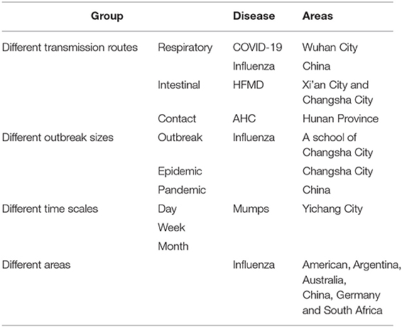
We compared and analyzed the goodness-of-fit and early warning of the LDE and GLDE models through COVID-19 data. To further generalize and test, we also classified other disease data into four categories from different perspectives: different transmission routes, different epidemic intensities, different time scales, and different areas to analyze the advantages and disadvantages of the models (Table 1). The research framework is shown in Figure 1.

TABLE 1

Table 1. Disease types and areas at different levels.

FIGURE 1

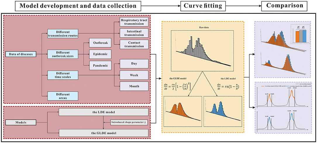
Figure 1. Research framework. GLDE, Generalized logistic differential equation; LDE, logistic differential equation; **p < 0.01; ***p < 0.001; EAW, epidemic accelerate week; WRW, warning remove week.

Epidemic Intensity Definition Based on Scales of Cases

We classified the influenza data as three epidemic intensities: outbreak, epidemic, and pandemic according to the definition from The Centers for Disease Control and Prevention (CDC) (36).

Epidemic refers to an increase, often sudden, in the number of cases of a disease above what is normally expected in that population in that area.

Outbreak carries the same definition of epidemic but is often used for a more limited geographic area.

Pandemic refers to an epidemic that has spread over several countries or continents, usually affecting a large number of people.

Model Development

The LDE Model

The LDE model was mainly used to describe population growth in the early stage and gradually was applied to the medical field (22). The differential equation is in Equation (1) (32), and its general solution is in Equation (2),

$\begin{array}{ll}\frac{dn}{dt}=rn(1-\frac{n}{N})& (1)\end{array}$

$\begin{array}{ll}n=\frac{N}{1+e^{-rt-c}}& (2)\end{array}$

where n is the cumulative number of cases, N is the upper line of the cumulative cases, r is the growth rate coefficient, and c is the constant generated when solving the LDE. dn/dt is the ratio of cumulative cases to time, which represents the change rate of cumulative cases n of infectious diseases at time t, and can also represent the model characteristics of new cases over time.

This model has three parameters, r, n, and N. The parameter values of r and N determine the specific shape of the model curve, and accurate parameter estimation will greatly improve fitting. According to the initial and critical conditions set, the critical value N at both ends of the LDE is known, and only the parameter r is unknown. However, in practical applications, the value of N is difficult to obtain because of the limitation of conditions; therefore, parameter estimation is sometimes required.

As the disease develops and immune barriers are built up in the population, the epidemic gradually reaches a stable state and the number of new cases gradually decreases until the epidemic is over. Therefore, the logistic model curve presents a “slow–fast–slow” trend, which shows an S shape. The point where the LDE model curve changes from slow to fast is called the inflection point. Doing the third-order derivation over Equation (2) to make the new equation equal to zero, and the result is Equation (3), whereas t₁ in Equation (4) is the inflection point of the curve of the LDE model, that is epidemic accelerate week.

$\begin{array}{ll}t=-c\pm 1.317/r& (3)\end{array}$

$\begin{array}{ll}{t}_1=-c-1.317/r& (4)\end{array}$

The GLDE Model

The LDE model requires data to be symmetrical, but data in some cases do not meet this requirement. Half a century ago, one classical logistic model was extended to allow S-shape to have more flexible curvature in the case of the asymmetric growth curve, so as to establish Richards' curve, that is, the GLDE model (37). After applying four parameters to the LDE model, there were five types of the GLDE model. The GLDE model with shape parameters can fit case data of various distribution types, so of interest in this study was the type of shape parameter introduced. The differential equation is in Equation (5), and the general solution is in Equation (6).

$\begin{array}{ll}\frac{dn}{dt}=\frac{rn}{\lambda }\left[1-{\left(\frac{n}{N}\right)}^{\lambda }\right]& (5)\end{array}$

$\begin{array}{ll}n=\frac{N}{{\left(1+e^{-rt+c}\right)}^{\frac{1}{\lambda }}}\left(N,\lambda ,r\rangle 0\right)& (6)\end{array}$

By calculating the first and second derivatives of the general solution of the GLDE and letting it be 0, we can obtain the unique inflection point. The growth rate of the GLDE model curve decreases with a decrease in nt, and the rate of decrease is related to the shape parameter λ. At first, the curve shape is concave, and the growth rate accelerates; after the inflection point, the curve is convex, the growth rate declines and finally tends to saturation. The GLDE model curve has four parameter values, r, n, N, and λ, and the shape of the curve is determined by the values of r, N, and λ.

As can be seen from the equation, when the shape parameters fall within the range of (0,1), the distribution is skewed to the left; when they are >1, the distribution is skewed to the right, and when they are equal to 1, the graph is symmetrically distributed, that is, the general logistics distribution.

Doing the third-order derivation over Equation (6) to make the new equation equal to zero, and the result is in Equation (7), whereas t₁ in Equation (8) is the inflection point of the curve of the GLDE model, that is epidemic accelerate week.

$\begin{array}{ll}t=-\frac{c-ln(\frac{3\pm \sqrt{5}}{2}\lambda )}{r}& (7)\end{array}$

$\begin{array}{ll}{t}_1=-\frac{c-ln(\frac{3-\sqrt{5}}{2}\lambda )}{r}& (8)\end{array}$

Parameter Estimation

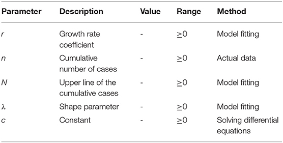
As shown in Table 2, there were five parameters, where r is the growth rate coefficient, n is the cumulative number of cases, N is the upper line of the cumulative cases, λ is the shape parameter, and c is the constant generated when solving the differential equations.

TABLE 2

Table 2. Definitions and sources of model parameter.

The corresponding parameters r, N, and λ are obtained by model fitting (see Supplementary File 1).

Model Fitting

Model fitting was performed on the number of cases. From the plots of the LDE model, the epidemic data in accordance with the LDE model, the plot of the number of cases over time should have a single-wave shape. Therefore, before fitting, the data must be divided into different segments, each consisting of a wave. The division of the data cycle could be determined according to the transmission characteristics of the diseases. For diseases with an obvious time cycle, it could be segmented according to their epidemic cycles. However, most infectious diseases did not have a specific cycle, or the cycle was not constant over time due to changes in influencing factors. Therefore, it was difficult to segment data according to a certain period of time.

Therefore, based on the assumptions of the LDE model and the characteristics of the curves, we segmented the period during the epidemic season (the interval between the first trough and the next trough). When two peaks with large intervals or fine tail segments appear, we removed these segments and fit only the peaks of the data. For data where peaks had bifurcations, we could choose whether to perform segmentation based on the size of the bifurcation. We compared the differences in the results by fitting the disease data of different disease types, different epidemic intensities, different time scales, and different areas to verify whether the two models can be used to fit the data of different types of epidemics and to explore their respective applicable conditions when dividing the “slow–fast–slow” period for infectious disease progression.

Epidemic Accelerate Time Prediction

The epidemic accelerate weeks of influenza data in each country were calculated by Equations (5) and (8), respectively. The epidemic accelerate time in 2019 was predicted according to the corresponding median from 2015 to 2018 and then compared to the reality to analyze the predicting effects.

Statistical Methods

Berkeley Madonna 8.3.18 software was used in the simulation of these models. Microsoft Excel 2019 software (Microsoft Corp, USA) was used for entering and managing related data and related mapping. The differential equation solving method was used with a fourth-order Runge-Kutta method with a tolerance of 0.001. The model convergence method was the least root mean square (LRMS) of the simulated data and the actual data. IBM SPSS Statistics for Windows, version 21.0 was used to calculate the coefficient of determination (R²) and p-values as the criterion to analyze and compare the goodness-of-fit of curves,

$\begin{array}{ll}{R}^2=\frac{S_{y^{\prime }}^2}{S_y^2}& (9)\end{array}$

where the ${\text{S}}_{{\text{y}}^{\text{′}}}^2$is the variance of the fitted value, the ${\text{S}}_{\text{y}}^2$ is the variance of the actual value. When p < 0.05, the closer R² was to 1, the better the goodness-of-fit of the model. The example data and Berkeley Madonna code are given in Supplementary Files 2, 3.

Results

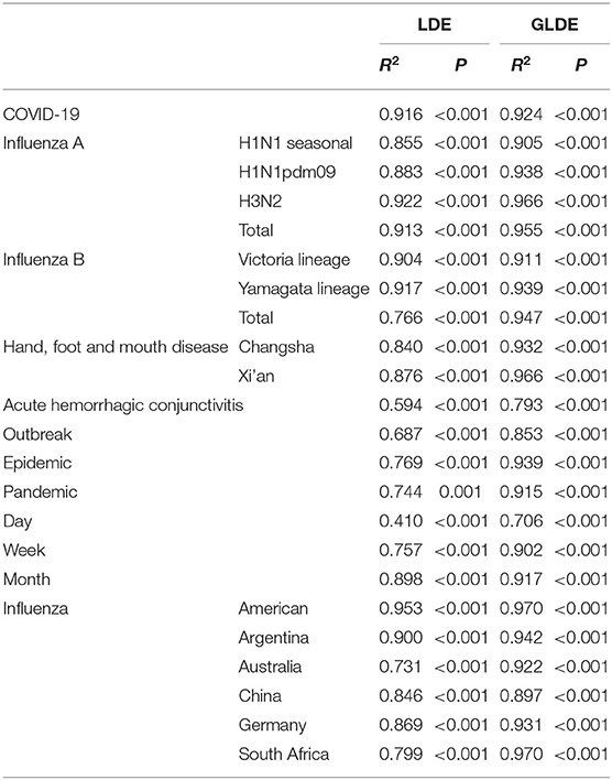
The fitting graphs showed that both models fitted the case data well, and the GLDE model was more suitable for the actual data. We performed LRMS analysis on the results of the two models separately and found that all results were statistically significant (p < 0.05). However, the R² calculated using the GLDE model to fit the data was higher (Table 3, Figure 2).

TABLE 3

Table 3. The results of goodness-of-fit.

FIGURE 2

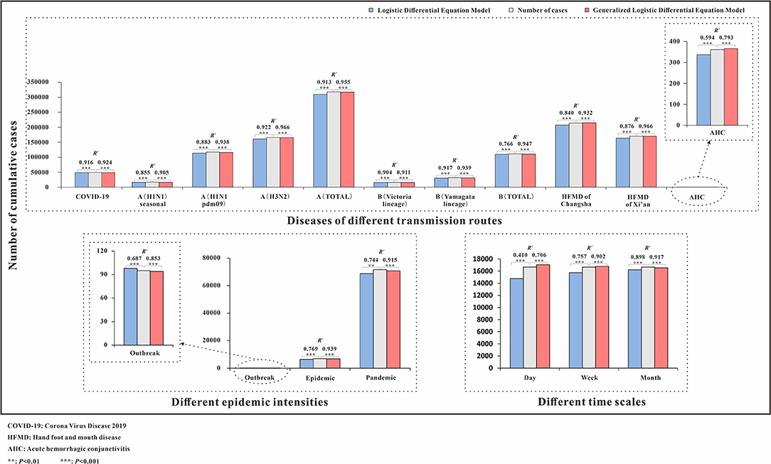
Figure 2. Number of cumulative cases and R² of logistic and generalized logistic differential equation models. COVID-19, coronavirus disease 2019; HFMD, hand, foot, and mouth disease; AHC, acute hemorrhagic conjunctivitis; **p < 0.01; ***p < 0.001.

COVID-19

The fitting diagram of COVID-19 in Wuhan city of the two methods is shown in Figure 3. The first wave of the COVID-19 pandemic in Wuhan lasted 106 days, and the cases showed an overall single-peak distribution so the data were not segmented. The number of cases began to decline after January 26, and there was an outlier on February 1. The R² test value fitted by the LDE model was 0.916 (p < 0.001) and the R² test value fitted by the GLDE model was 0.905 (p < 0.001).

FIGURE 3

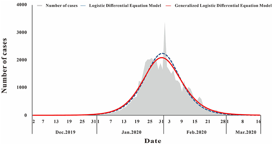
Figure 3. Curve fitting results of logistic and generalized logistic differential equation models of COVID-19.

According to Equations 5, 8, the epidemic acceleration time of COVID-19 in Wuhan calculated by the LDE model and the GLDE model was January 23 and January 24, respectively, and the LDE model was slightly earlier than the GLDE model.

Other Diseases

Infectious Diseases With Different Transmission Routes

The fitting diagram of A (H1N1) seasonal, A (H1N1pdm09), A (H3N2), and the total number of influenza A infections among respiratory infectious diseases are shown in Figures 4a–d. The figure showed how disease peaks of different subtypes of influenza differed. The A (H1N1) seasonal data from the 48th week of 2010 to the 46th week of 2015 were 0. After abandoning these data, the remaining data were divided into 14 segments according to the epidemic curve. There were obvious fluctuations in the two peaks in 2009 and 2010. The epidemic curve showed that there were more cases in 2001 and 2005 than in 2009. The highest number of cases per week was 355, and it appeared in week 8 of 2009. The R² test value fitted by the LDE model was 0.855 (p < 0.001), and the R² test value fitted by the GLDE model was 0.905 (p < 0.001). In the influenza A (H1N1pdm09) data, the data from the 1st week of 2001 to the 17th week of 2009 were all zero. Therefore, the fitting data starting from the 18th week of 2009 were divided into eight segments. The epidemic curve showed that the number of cases in 2009 reached maximum, with an obvious wave peak. The highest number of cases per week reached 5,383, which occurred in the 39th week of 2009. At other times, the number of cases was low and sporadic. The R² test value fitted by the LDE was 0.883 (p < 0.001), and the R² test value fitted by the GLDE was 0.938 (p < 0.001). The distribution of influenza A (H3N2) data showed that it could be divided into 26 segments. The peaks in 2007 and 2012 were different from the traditional peaks, and they were fluctuated, with a small fluctuation at the peak. In 2001, from 36 weeks in 2005 to 36 weeks in 2006, and from 14 to 27 weeks in 2011, the number of cases was relatively small, and the wave peak was not distinct. The highest number of cases per week was 2,747, which occurred in the fourth week of 2015. The R² test value fitted by the LDE model was 0.922 (p < 0.001), and the R² test value fitted by the GLDE model was 0.966 (p < 0.001). The distribution map of the influenza A summary data showed that it could be divided into 28 segments. The number of cases after the 28th week of 2009 increased significantly compared with before, and the peak in 2012 was more flat; the highest number of cases per week was 7,280, which occurred in the 37th week of 2009. The R² test value fitted by the LDE model was 0.913 (p < 0.001), and the R² test value fitted by the GLDE model was 0.955 (p < 0.001).

FIGURE 4

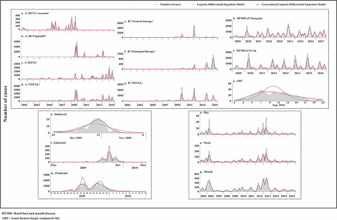
Figure 4. Curve fitting results of logistic and generalized logistic differential equation models. (a) A (H1N1) seasonal, (b) A (H1N1pdm09), (c) A (H3N2), (d) A (Total), (e) B (Victoria lineage), (f) B (Yamagata lineage), (g) B (Total), (h) HFMD of Changsha, (i) HFMD of Xi'an, (j) AHC, (k) Outbreak, (l) Epidemic, (m) Pandemic, (n) Day, (o) Week, and (p) Month. HFMD, Hand foot and mouth disease; AHC, Acute hemorrhagic conjunctivitis.

The fitting graphs of B (Victoria lineage), B (Yamagata lineage), and the total number of B types are shown in Figures 4e–g. B (Victoria lineage) influenza data, which could be divided into eight segments according to the epidemic curve, showed that cases began to appear in the 20th week of 2008. The highest number of weekly cases reached 1,041, which occurred in week 8 of 2012. The R² test value fitted by the LDE model was 0.904 (p < 0.001), and the R² test value fitted by the GLDE model was 0.911 (p < 0.001). The B (Yamagata lineage) influenza data, which could be divided into 12 segments according to the epidemic curve, with four obvious peaks, showed that the cases appeared in week 20 of 2008. Among them, the 2014 and 2015 peaks were different from the traditional peaks, and all were serrated, that was, had two peak values. The highest number of cases per week reached 1,055, which occurred in week 10 of 2015. The R² test value fitted by the LDE model was 0.917 (p < 0.001), and the R² test value fitted by the GLDE model was 0.939 (p < 0.001). The distribution map of the influenza B summary data showed that it could be divided into 17 segments, among which four relatively dense peak groups appeared after 2010. In contrast to the traditional wave peaks, they were serrated. The highest number of cases per week was 2,630, which occurred in week 8 of 2012. The R² test value fitted by the LDE model was 0.766 (p < 0.001), and the R² test value fitted by the GLDE model was 0.947 (p < 0.001).

The fitting diagrams of HFMD in Xi'an city and Changsha City among enteric diseases are shown in Figures 4h,i, and the epidemic curves showed that the two cities annually presented double seasonal peaks. The epidemic curve of HFMD in Xi'an City could be divided into 14 segments. From 2009 to 2015, the peak in the first half was significantly higher than in the second, and the two peaks in 2016 were not significantly different. The highest number of cases per week reached 2,013, which occurred in week 23 of 2015. The R² test value fitted by the LDE model was 0.876 (p < 0.001), and the R² test value fitted by the GLDE was 0.966 (p < 0.001). The epidemic curve of HFMD in Changsha City could be divided into 19 segments. The distribution in 2015 differed from other years, not being an obvious bimodal distribution. Moreover, the first peaks in 2010, 2014, and 2016 differed from the traditional wave peak, all being serrated. The highest number of cases per week reached 2,163, which occurred in week 17 of 2014. The R² test value fitted by the LDE model was 0.840 (p < 0.001), and the R² test value fitted by the GLDE model was 0.932 (p < 0.001).

The fitting diagram of AHC in contact infectious diseases is shown in Figure 4j, and the data were not segmented. The R² test value fitted by the LDE model was 0.594 (p < 0.001), and the R² test value fitted by the GLDE model was 0.793 (p < 0.001).

Infectious Diseases With Different Epidemic Intensities

The fitting graphs of the outbreak, epidemic, and pandemic are shown in Figures 4k–m. The outbreak data fitting results showed that the goodness-of- fit of the GLDE model (R² = 0.853, p < 0.001) was better than that of the LDE model (R² = 0.687, p < 0.001). The epidemic data were fitted with the flu data of Changsha City as an example, and the epidemic curve could be divided into seven segments. The R² test value fitted by the LDE model was 0.769 (p < 0.001), and the R² test value fitted by the GLDE was 0.939 (p < 0.001). The pandemic data contained the 2009 and 2010 influenza data of China as an example, and the epidemic curve could be divided into four segments. The R² test value fitted by the LDE model was 0.744 (p < 0.001), and the R² test value fitted by the GLDE model was 0.915 (p < 0.001).

Infectious Disease From Different Time Scales

We used two methods to fit the mumps data from Yichang City with time scales of days, weeks, and months. The results are shown in Figures 4n–p. When taking days as the time scale, it could be divided into 21 segments according to the epidemic curve. Among them, there were more cases in 2006 and 2013 with the highest number of daily cases being 56, which occurred on 13 May 2013. The R² test value fitted by the LDE model was 0.410 (p < 0.001), and the R² test value fitted by the GLDE model was 0.706 (p < 0.001). When taking weeks as the time scale, it could be divided into 21 segments according to the epidemic curve. The highest number of weekly cases was 208, which occurred in week 19 of 2013. The R² test value fitted by the LDE model was 0.757 (p < 0.001), and the R² test value fitted by the GLDE model was 0.902 (p < 0.001). When the month was taken as the time scale, it could be divided into 15 segments according to the epidemic curve. The highest number of monthly cases was 686, which occurred in May 2013. The R² test value fitted by the LDE model was 0.898 (p < 0.001), and the R² test value fitted by the GLDE model was 0.917 (p < 0.001).

Infectious Diseases in Different Areas

The fitting diagram of influenza in each country is shown in Figure 5. Influenza data in Argentina were divided into 5 segments according to the epidemic curve. The highest number of weekly cases was 1,072, which occurred in week 22 of 2016. The R² test value fitted by the LDE model was 0.9 (p < 0.001) and the R² test value fitted by the GLDE model was 0.942 (p < 0.001). Influenza data in Australia were divided into 6 segments according to the epidemic curve. The highest number of weekly cases was 1,002, which occurred in week 26 of 2019. The R² test value fitted by the LDE model was 0.731 (p < 0.001) and the R² test value fitted by the GLDE model was 0.922 (p < 0.001). Influenza data in China were divided into 8 segments according to the epidemic curve. The highest number of weekly cases was 8,426, which occurred in week 3 of 2019. The R² test value fitted by the LDE model was 0.846 (p < 0.001), and the R² test value fitted by the GLDE model was 0.897 (p < 0.001). Influenza data in Germany were divided into 5 segments according to the epidemic curve. The highest number of weekly cases was 292, which occurred in week 9 of 2018. The R² test value fitted by the LDE model was 0.869 (p < 0.001), and the R² test value fitted by the GLDE model was 0.931 (p < 0.001). Influenza data in South Africa were divided into 6 segments according to the epidemic curve. The highest number of weekly cases was 197, which occurred in week 24 of 2019. The R² test value fitted by the LDE model was 0.799 (p < 0.001) and the R² test value fitted by the GLDE model was 0.875 (p < 0.001). Influenza data in America were divided into 6 segments according to the epidemic curve. The highest number of weekly cases was 26,386, which occurred in week 5 of 2018. The R² test value fitted by the LDE model was 0.953 (p < 0.001), and the R² test value fitted by the GLDE model was 0.97 (p < 0.001).

FIGURE 5

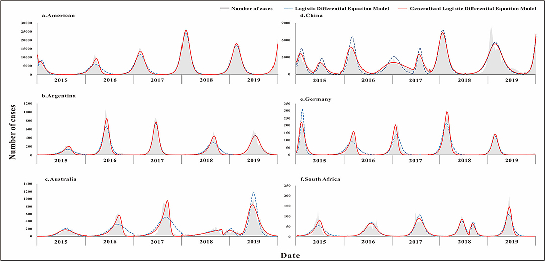
Figure 5. Curve fitting results of logistic and generalized logistic differential equation models in different areas. (a) American, (b) Argentina, (c) Australia, (d) China, (e) Germany, and (f) South Africa.

The results showed that the goodness-of-fit of the GLDE model was all better than that of the LDE model in each country, and the cumulative cases and the R² values of the goodness-of-fit test are shown in Figure 6.

FIGURE 6

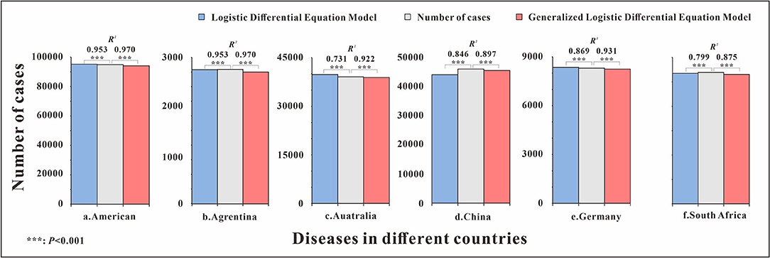
Figure 6. Number of cumulative cases and R² of logistic and generalized logistic differential equation models in different areas. ***p < 0.001.

Determination of the Early Warning Week

The parameters were plugged into Equations 5, 8 to calculate each country's annual epidemic acceleration week. The last segment data of the United States and China in 2019 were not a complete wave, and it was not possible to calculate the warning week, so it was omitted. The epidemic acceleration weeks of influenza in each country are shown in Figure 7. There was only one incidence peak (in winter) in two countries (United States and Germany). There was only one incidence peak (in summer) in two countries (Argentina and South Africa), and there was also a small peak (in autumn) in South Africa in 2018. There was only one incidence peak (in autumn) in Australia, and there was also a small peak (in winter) in 2018. In addition to the winter peak, there was also a summer peak in 2015 and 2017 in China, and there was only one winter peak in the other years. The parametric test results showed that the calculated t-test statistic was −0.236 with a corresponding p-value of 0.025, and the difference was statistically significant, rejecting the assumption that the EAW calculated by the LDE and GLDE models was the same. So, it can be considered that EAW calculated by the LDE model was earlier than the GLDE model.

FIGURE 7

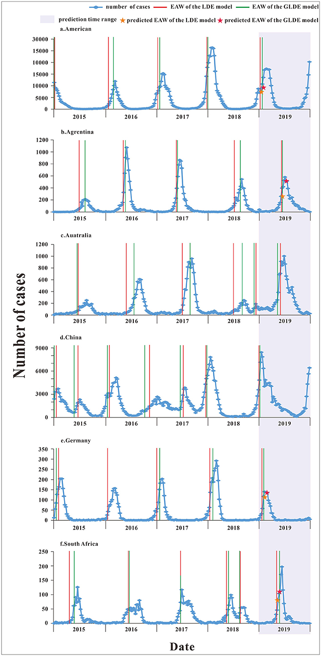
Figure 7. The epidemic acceleration week of logistic and generalized logistic differential equation models in different areas. (a) American, (b) Argentina, (c) Australia, (d) China, (e) Germany, and (f) South Africa.

According to the corresponding median from 2015 to 2018, the epidemic acceleration time in 2019 was predicted. Because the data were divided according to the epidemic curve of the disease, the specific starting time of the epidemic in each year was different, which may affect the prediction of the epidemic accelerate week, so we excluded prediction values that were not in the actual year. For example, in Australia, the number of cases started to increase later in 2019 late than in other years; and in China, the number of cases began to increase in late 2018 and reached relatively high in early 2019, and these two predicted values differed greatly from the actual values, so they were omitted. The specific numerical value of the epidemic accelerate week of each country are shown in Supplementary File 4.

Discussions

Feasibility Analysis of Models

The curves of the LDE model are sigmoidal or antisigmoidal (increasing or decreasing). When the second and third derivatives of the model equation are solved, two inflection points and one peak point can be obtained. The two inflection points divide the LDE model curve into the growth, rapid growth, and slow growth phases, which respectively correspond to the beginning, peak, and end of peak periods of the epidemic curve (29). The LDE model is suitable for symmetric data and has been widely used in various infectious disease prevention, control, and early warning studies (28, 29, 38, 39). The curves of the GLDE model are similar to those of the LDE model and can be divided into the same three periods. However, due to the introduction of shape parameters, the GLDE model is suitable for symmetric data and can be used to fit asymmetric data. Currently, some studies use the GLDE model for data fitting (38).

Advantages and Disadvantages Analysis of the Models

From the perspective of model derivation, in theory, both models can be used to predict the development trend of infectious diseases, but the applicable conditions are different and there are advantages and disadvantages in the fitting of epidemic data. The LDE model is simple, understandable, and the second derivative can be used to determine the early warning time. However, it has several disadvantages, for example, the model's inflexibility, poor fit of asymmetric or fine-tailed distribution data, and unsuitability for long-term prediction. The GLDE model can be used for epidemic data of different distribution types by introducing shape parameters, but the calculation of epidemic inflection points is more complex. The comparison of the LDE and GLDE models is shown in Table 4.

TABLE 4

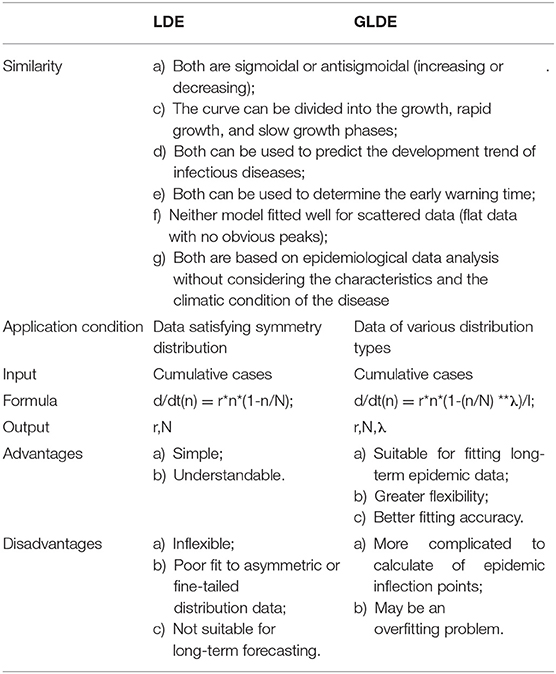
Table 4. Comparison of logistic differential equation (LDE) and generalized logistic differential equation (GLDE).

The Difference of Model Fitting Results

Both LDE and GLDE models fitted the epidemic curve of the COVID-19 well, and correlations between fitting data and actual data were found (R²> 0.9, p < 0.05), and the goodness-of- fit of the GLDE model was better than that of the LDE model. The COVID-19 epidemic curve was asymmetrical, and the GLDE model added shape parameters to make it more suitable for fitting such data.

Observing the epidemic curves of infectious diseases with different transmission routes, we found that the regularity of the epidemic curve of influenza in respiratory infectious diseases was not distinct. There were many abnormal values and abnormal peaks. In enteric diseases, the peaks of HFMD were relatively uniform and had a notable regularity, with double seasonal peaks in spring and early winter (40–43). Among contagious infectious diseases, the AHC peak was also slightly different from the traditional peak.

There were significant outliers in A (H1N1) seasonal 2006, A (H1N1pdm09) 2009, and the total number of influenza cases in 2006, B (Yamagata lineage), 2010, and 2011. Only the outlier segmentation point of B (Yamagata lineage) in 2011 was used, and the other outliers were at their peak. The goodness-of-fit test showed that both methods could be used to data fit the outliers and, except for the LDE model in the form of B (Yamagata lineage) in 2011, the GLDE model fitted the remaining exceptions better. The derivation process of the LDE and GLDE models indicates that the models are highly stable. Individual values do not affect the overall shape of the disease epidemic curve due to long-term dispersal fluctuations. Therefore, the appearance of individual outliers does not affect the fit. Due to shape parameters being introduced, the GLDE may better fit the emergent outliers.

For data with a bifurcated peak, if it was not obvious, we ignored the bifurcation point and directly fit the entire segment, such as the thirteenth segment of A (H1N1) seasonal data. If it was obvious, we used the bifurcation point to segment, such as in the sixth and seventh segments of A (H1N1). The test results confirmed that with the two methods, the data could be fitted, but the GLDE model fitted better. This may be because the GLDE model introduces shape parameters that can be used for irregular data fitting.

In addition, there were many flat data with no obvious peaks in the influenza data, and the results of the goodness-of-fit tests showed that neither model fitted well for such scattered data. The sixth segment data of A (H1N1) seasonal cannot be fitted with the GLDE model, and the 8th and 10th segments data of B (Yamagata lineage) cannot be fitted with the LDE model. This may be because the assumption provided by the LDE model was that the data should be continuous and the data characteristics should be distributed. The “0” value often appeared in scattered data; therefore, the LDE and GLDE models were less commonly used for fitting scattered data. This is why outbreak, epidemic, and pandemic data were chosen when fitting data from different epidemic intensities. The test results also showed that the GLDE fitted well. The epidemic curve showed that the data of the three epidemic intensities were asymmetrically distributed and that the model better fitted asymmetrical distribution data after introducing the shape parameters.

When the same data were integrated into different time scales, the fitting results showed that both models produced the best goodness-of-fit using monthly data, rather than weekly and daily data. When observing the epidemic curve, we found that the monthly data distribution was smoother, which indicated that the data distribution somewhat affected the fitting. In addition, the GLDE model fitted better than the LDE model at different time scales. We speculate that the GLDE is more suitable for data with flat fluctuations after the introduction of the shape parameters.

When fitting cases data in different countries, the GLDE model fitted better than the LDE model. The pattern of the epidemic curves of influenza differed among countries, which was associated with different climatic environments, geographical conditions, population density, different traditions, and preventive and control measures (23).

In summary, although the logistic model is simple and rough, it accurately fits the disease data and describes the epidemic dynamics. The LDE and GLDE models can be used to fit epidemic data at different levels. The GLDE model fits the actual data more accurately than the LDE model, and the same result can be seen in Pelinovsky's research (23). The approximation accuracy increased significantly using the GLDE model than the LDE model, including the data for which the simple LDE model was not suitable. Studies (44, 45) also found that the introduction of the shape parameter within the GLDE model significantly improved the adjustment compared with the LDE model. Due to the significant contribution of the shape parameter, the GLDE model can not only better approximate the dynamics of data but can also capture the real data better. As the LDE model has limitations regarding the requirements for a skewed data distribution, in addition, over a long period, the parameters are not stable due to the interference factors changing, which render the LDE model unsuitable for fitting long-term epidemic data. The GLDE model is more suitable for fitting various distribution data and has better goodness-of-fit than LDE model, and this improvement is partly due to the additional parameter based on the LDE model. In fact, it is the result of the general statistical rule that the increase of the number of approximate curve parameters leads to the increase of the coefficient of determination (23). Therefore, the GLDE model may have the problem of overfitting. In practical application, we need to select an appropriate model based on the specific distribution of data. For asymmetrically distributed disease data, the GLDE model demonstrates greater flexibility and better fitting accuracy.

The Difference of Determination of the Early Warning Week

The epidemic acceleration time of COVID-19 in Wuhan city calculated by the LDE and GLDE models was January 23 and January 24, respectively. The actual time of lockdown of Wuhan was January 23, and the calculation result of the LDE model was closer to reality. The LDE model can accurately calculate the epidemic accelerate time and then determine the critical time of the epidemic, which has important reference significance for relevant departments to take prevention and control measures, especially in major public health events.

Both LDE and GLDE models can well characterize the patterns of influenza epidemics in different countries and calculate the annual acceleration weeks. In general, The EAW calculated by the LDE model is slightly earlier than that calculated by the GLDE model. The advantages and disadvantages of the LDE and GLDE models in early warning need further study.

The fitting principle of logistic models is simple, and the calculation efficiency is high (46). The current COVID-19 pandemic is a scenario for such models that are of obvious significance (44). It can provide a rapid and timely description of epidemic dynamics in the early stage, using simple indicators, when the epidemiological characteristics of the diseases are unclear (2). When other factors become widespread, such as the difference between public health interventions and input cases abroad, the transmission of infectious diseases may complicate the research methods, and the logistic models may not be enough (47). However, it is still an important tool in modeling epidemics as it accurately estimates the critical points of the epidemic, allowing public health workers and managers to better understand the whole process of epidemic development and formulate scientific prevention and control measures (48).

Combined with the actual data of COVID-19 data and other infectious diseases, a comparative study was conducted using the LDE and GLDE models for infectious disease epidemic simulation and early warning. The scope of our study included infectious diseases with different transmission routes (respiratory tract transmission, enteric transmission, and contact transmission), different epidemic intensities (outbreak, epidemic, and pandemic), different time scales (day, week, and month), and different areas. Using R², an indicator that reflects the goodness-of-fit, we found that the GLDE model provided a more accurate fit of data than the LDE model. Through the parametric test, we found that the LDE model provided earlier early warning week than the GLDE model. Therefore, we have reason to believe that the GLDE model is more advantageous in asymmetric infectious disease data simulation, however, its advantages of quantification in the middle and late stages of the epidemic, prediction, and early warning need to be further studied. In practice, we can choose appropriate models for disease prediction and early warning according to the region and the severity of the disease.

Conclusion

The GLDE model provides more accurate goodness-of-fit to the data than the LDE model. The GLDE model is able to handle asymmetric data by introducing shape parameters that allow it to fit data with various distributions. The LDE model provides the earlier epidemic acceleration week than the GLDE model. We conclude that the GLDE model is more advantageous in asymmetric infectious disease data simulation.

Data Availability Statement

The datasets used and analyzed during the current study are available from Zhuoyang Li (ODA1NDkzOTI5JiN4MDAwNDA7cXEuY29t) on reasonable request.

Author Contributions

YS, BZ, HZ, JL, KL, Y-CC, and TC made substantial contributions to conception and design and critically revised the manuscript for important intellectual content. YB, HZ, JL, and KL collected data. ZL, SL, JR, YB, YS, BZ, HZ, JL, KL, Y-CC, and TC conceived the experiments. ZL, SL, JR, YB, BD, QC, YZ, LL, SY, WL, and SZ conducted experiments and analyzed results. ZL, SL, JR, and YB wrote the manuscript. All authors read and approved the final manuscript.

Funding

This study was supported by the Bill & Melinda Gates Foundation (INV-005834). The funder had no role in study design, data collection and analysis, decision to publish, or preparation of the manuscript.

Conflict of Interest

The authors declare that the research was conducted in the absence of any commercial or financial relationships that could be construed as a potential conflict of interest.

Publisher's Note

All claims expressed in this article are solely those of the authors and do not necessarily represent those of their affiliated organizations, or those of the publisher, the editors and the reviewers. Any product that may be evaluated in this article, or claim that may be made by its manufacturer, is not guaranteed or endorsed by the publisher.

Acknowledgments

We thank the support from the Undergraduate Innovation Practice Platform of the School of Public Health, Xiamen University.

Supplementary Material

The Supplementary Material for this article can be found online at: https://www.frontiersin.org/articles/10.3389/fpubh.2022.813860/full#supplementary-material

Abbreviations

LDE, logistic differential equation; GLDE, generalized logistic differential equation; COVID-19, coronavirus disease 2019; SARS, severe acute respiratory syndrome; A/H1N1, influenza A virus subtype H1N1; EVD, Ebola virus disease; SIR, susceptible-infective-removed; SEIAR, Susceptible-exposed-infective-asymptomatic-removed; HFMD, hand, foot, and mouth disease; AHC, acute hemorrhagic conjunctivitis; CDC, The Center for Disease Control and Prevention; WHO, World Health Organization; LRMS, the least root mean square; R², the coefficient determination.

References

1. Wu K, Darcet D, Wang Q, Sornette D. Generalized logistic growth modeling of the COVID-19 outbreak: comparing the dynamics in the 29 provinces in China and in the rest of the world. Nonlinear Dynam. (2020) 101:1561–81. doi: 10.1007/s11071-020-05862-6

PubMed Abstract | CrossRef Full Text | Google Scholar

2. Zou Y, Pan S, Zhao P, Han L, Wang X, Hemerik L, et al. Outbreak analysis with a logistic growth model shows COVID-19 suppression dynamics in China. PLoS ONE. (2020) 15:e0235247. doi: 10.1371/journal.pone.0235247

PubMed Abstract | CrossRef Full Text | Google Scholar

3. Sanyaolu AO, Okorie C, Hosein ZA, Patidar R, Marinkovic A, JIDR Treatment. Global pandemicity of COVID-19: Situation Report as of June 9, 2020. Infect Dis Res Treat. (2021) 14:1–8. doi: 10.1177/1178633721991260

PubMed Abstract | CrossRef Full Text | Google Scholar

4. Yan WR, Nie SF, Xu B, Dong HJ, Palm L, Diwan VK. Establishing a web-based integrated surveillance system for early detection of infectious disease epidemic in rural China: a field experimental study. BMC Med Inform Decis Mak. (2012) 12:4. doi: 10.1186/1472-6947-12-4

PubMed Abstract | CrossRef Full Text | Google Scholar

5. Fraser C, Donnelly CA, Cauchemez S, Hanage WP, Van Kerkhove MD, Hollingsworth TD, et al. Pandemic potential of a strain of influenza A (H1N1): early findings. Science. (2009) 324:1557–61. doi: 10.1126/science.1176062

PubMed Abstract | CrossRef Full Text | Google Scholar

6. Yen MY, Chiu AW, Schwartz J, King CC, Lin YE, Chang SC, et al. From SARS in 2003 to H1N1 in 2009: lessons learned from Taiwan in preparation for the next pandemic. J Hosp Infect. (2014) 87:185–93. doi: 10.1016/j.jhin.2014.05.005

PubMed Abstract | CrossRef Full Text | Google Scholar

7. Kwok KO, Davoudi B, Riley S, Pourbohloul B. Early real-time estimation of the basic reproduction number of emerging or reemerging infectious diseases in a community with heterogeneous contact pattern: using data from Hong Kong 2009 H1N1 Pandemic Influenza as an illustrative example. PLoS ONE. (2015) 10:e0137959. doi: 10.1371/journal.pone.0137959

PubMed Abstract | CrossRef Full Text | Google Scholar

8. Hsiang S, Allen D, Annan-Phan S, Bell K, Bolliger I, Chong T, et al. The effect of large-scale anti-contagion policies on the COVID-19 pandemic. Nature. (2020) 584:262–7. doi: 10.1038/s41586-020-2404-8

PubMed Abstract | CrossRef Full Text | Google Scholar

9. Tong MX, Hansen A, Hanson-Easey S, Cameron S, Xiang J, Liu Q, et al. Infectious diseases, urbanization and climate change: challenges in future China. Int J Environ Res Public Health. (2015) 12:11025–36. doi: 10.3390/ijerph120911025

PubMed Abstract | CrossRef Full Text | Google Scholar

10. Li DF, Shen T, Zhang Y, Wu HY, Gao LD, Wang DM, et al. [Strategy for prevention and control of imported infectious disease]. Zhonghua Liu Xing Bing Xue Za Zhi. (2018) 39:1291–7. doi: 10.3760/cma.j.issn.0254-6450.2018.10.001

PubMed Abstract | CrossRef Full Text | Google Scholar

11. Chowell G, Hincapie-Palacio D, Ospina J, Pell B, Tariq A, Dahal S, et al. Using phenomenological models to characterize transmissibility and forecast patterns and final burden of zika epidemics. PLoS Curr. (2016) 8:ecurrents.outbreaks.f14b2217c902f453d9320a43a35b9583. doi: 10.1371/currents.outbreaks.f14b2217c902f453d9320a43a35b9583

PubMed Abstract | CrossRef Full Text | Google Scholar

12. Mandal S, Bhatnagar T, Arinaminpathy N, Agarwal A, Chowdhury A, Murhekar M, et al. Prudent public health intervention strategies to control the coronavirus disease 2019 transmission in India: a mathematical model-based approach. Indian J Med Res. (2020) 151:190–9. doi: 10.4103/ijmr.IJMR_504_20

PubMed Abstract | CrossRef Full Text | Google Scholar

13. Chowell G, Sattenspiel L, Bansal S, Viboud C. Mathematical models to characterize early epidemic growth: a review. Phys Life Rev. (2016) 18:66–97. doi: 10.1016/j.plrev.2016.07.005

PubMed Abstract | CrossRef Full Text | Google Scholar

14. Havumaki J, Meza R, Phares CR, Date K, Eisenberg MC. Comparing alternative cholera vaccination strategies in Maela refugee camp: using a transmission model in public health practice. BMC Infect Dis. (2019) 19:1075. doi: 10.1186/s12879-019-4688-6

PubMed Abstract | CrossRef Full Text | Google Scholar

15. Driedger SM, Cooper EJ, Moghadas SM. Developing model-based public health policy through knowledge translation: the need for a 'Communities of Practice'. Public Health. (2014) 128:561–7. doi: 10.1016/j.puhe.2013.10.009

PubMed Abstract | CrossRef Full Text | Google Scholar

16. Kim S, Lee J, Jung E. Mathematical model of transmission dynamics and optimal control strategies for 2009 A/H1N1 influenza in the Republic of Korea. J Theor Biol. (2017) 412:74–85. doi: 10.1016/j.jtbi.2016.09.025

PubMed Abstract | CrossRef Full Text | Google Scholar

17. Wu JT, Leung K, Leung GM. Nowcasting and forecasting the potential domestic and international spread of the 2019-nCoV outbreak originating in Wuhan, China: a modelling study. Lancet. (2020) 395:689–97. doi: 10.1016/S0140-6736(20)30260-9

PubMed Abstract | CrossRef Full Text | Google Scholar

18. Batista M. Estimation of the final size of the second phase of the coronavirus epidemic by the logistic model. medRxiv [Preprint]. (2020). doi: 10.1101/2020.03.11.20024901

CrossRef Full Text | Google Scholar

19. Aviv-Sharon E, Aharoni A. Generalized logistic growth modeling of the COVID-19 pandemic in Asia. Infect Dis Model. (2020) 5:502–9. doi: 10.1016/j.idm.2020.07.003

PubMed Abstract | CrossRef Full Text | Google Scholar

20. Liang K. Mathematical model of infection kinetics and its analysis for COVID-19, SARS and MERS. Infect Genet Evol. (2020) 82:104306. doi: 10.1016/j.meegid.2020.104306

PubMed Abstract | CrossRef Full Text | Google Scholar

21. Sonnino G. Dynamics of the COVID-19-comparison between the theoretical predictions and real data. arXiv [Preprint]. (2020). arXiv:2003.13540.

22. Verhulst P-F. Notice sur la loi que la population suit dans son accroissement. Corresp Math Phys. (1838) 10:113–26.

23. Pelinovsky E, Kurkin A, Kurkina O, Kokoulina M, Epifanova A. Logistic equation and COVID-19. Chaos Soliton Fract. (2020) 140:110241. doi: 10.1016/j.chaos.2020.110241

PubMed Abstract | CrossRef Full Text | Google Scholar

24. Cássaro F. Pires LJT. Can we predict the occurrence of COVID-19 cases? Considerations using a simple model of growth. Sci Total Environ. (2020) 728:138834. doi: 10.1016/j.scitotenv.2020.138834

PubMed Abstract | CrossRef Full Text | Google Scholar

25. Tappe S. A simple mathematical model for the evolution of the corona virus. arXiv [Preprint]. (2020). arXiv:2003.09477.

26. Vasconcelos GL, Brum AA, Almeida FAG, Macedo AMS, Duarte-Filho GC, Ospina R. Standard and anomalous waves of COVID-19: A multiple-wave growth model for epidemics. Braz J Phys. (2021) 51:1867–83. doi: 10.1007/s13538-021-00996-3

CrossRef Full Text | Google Scholar

27. Wang XS, Wu J, Yang Y. Richards model revisited: validation by and application to infection dynamics. J Theor Biol. (2012) 313:12–9. doi: 10.1016/j.jtbi.2012.07.024

PubMed Abstract | CrossRef Full Text | Google Scholar

28. Zhang XX, Liu RC, Xie Z, Li YM, Chen SL, Zhao J, et al. Logistic differential equation model applying in the study of HFMD warning. China Trop Med. (2015) 15:942–61. doi: 10.13604/j.cnki.46-1064/r.2015.08.10

CrossRef Full Text | Google Scholar

29. Zhang XX, Chen TM, Liu RC, Wei H, Xie Z, Li YM, et al. Application of Logistic model in simulating influenza A (H1N1) pandemic. Practical Prev Med. (2014) 21:1052–5. doi: 10.3969/j.issn.1006-3110.2014.09.009

CrossRef Full Text | Google Scholar

30. Zhang XX, Liu RC, Xie Z, Chen TM. Early warning of infectious diarrhea by using logistic differential equation model. J Med Pest Control. (2017) 33:913–5. doi: 10.7629/yxdwfz201709001

CrossRef Full Text | Google Scholar

31. Xie Z, Chen TM, Lin X, Chen SL, Zao J, Liu RC. Establishment and application of Logistic differential equation model in the early warning of mumps. J Public Health Prev Med. (2015) 26:14–7.

32. Rui J, Luo KW, Chen QP, Zhang DX, Zhao QL, Zhang YH, et al. Early warning of hand, foot, and mouth disease transmission: a modeling study in mainland, China. PLoS Negl Trop Dis. (2021) 15:e0009233. doi: 10.1371/journal.pntd.0009233

PubMed Abstract | CrossRef Full Text | Google Scholar

33. Lin SN, Rui J, Chen QP, Zhao B, Yu SS, Li ZY, et al. Effectiveness of potential antiviral treatments in COVID-19 transmission control: a modelling study. Infect Dis Poverty. (2021) 10:53. doi: 10.1186/s40249-021-00835-2

PubMed Abstract | CrossRef Full Text | Google Scholar

34. Yang D, Liu R, Ye L, Hu Q, Rui J, Zhou Y, et al. Hand, foot, and mouth disease in Changsha City, China, 2009-2017: A new method to analyse the epidemiological characteristics of the disease. Infect Dis. (2020) 52:39–44. doi: 10.1080/23744235.2019.1675902

PubMed Abstract | CrossRef Full Text | Google Scholar

35. Zhang S, Hu Q, Deng Z, Hu S. Chen TJSR. Transmissibility of acute haemorrhagic conjunctivitis in small-scale outbreaks in Hunan Province, China. Sci Rep. (2020) 10:119. doi: 10.1038/s41598-019-56850-9

PubMed Abstract | CrossRef Full Text | Google Scholar

36. Dicker RC, Coronado F, Koo D, Parrish RG. Principles of epidemiology in public health practice. 3rd ed. In: An Introduction to Applied Epidemiology and Biostatistics. Atlanta, GA: US Department of Health and Human Services (2006).

37. Richards FJ. A flexible growth function for empirical use. J Exp Bot. (1959) 10:290–301. doi: 10.1093/jxb/10.2.290

CrossRef Full Text | Google Scholar

38. Liang R, Lu Y, Qu X, Su Q, Li C, Xia S, et al. Prediction for global African swine fever outbreaks based on a combination of random forest algorithms and meteorological data. Transbound Emerg Dis. (2020) 67:935–46. doi: 10.1111/tbed.13424

PubMed Abstract | CrossRef Full Text | Google Scholar

39. Pang FR, Luo QH, Hong XQ, Wu B, Zhou JH, Zha WT, et al. The study on the early warning period of varicella outbreaks based on logistic differential equation model. Epidemiol Infect. (2019) 147:e70. doi: 10.1017/S0950268818002868

PubMed Abstract | CrossRef Full Text | Google Scholar

40. Zhuang ZC, Kou ZQ, Bai YJ, Cong X, Wang LH Li C, et al. Epidemiological research on hand, foot, and mouth disease in mainland China. Viruses. (2015) 7:6400–11. doi: 10.3390/v7122947

PubMed Abstract | CrossRef Full Text | Google Scholar

41. Han Y, Chen Z, Zheng K, Li X, Kong J, Duan X, et al. Epidemiology of Hand, foot, and mouth disease before and after the introduction of enterovirus 71 vaccines in Chengdu, China, 2009-2018. Pediatr Infect Dis J. (2020) 39:969–78. doi: 10.1097/INF.0000000000002745

PubMed Abstract | CrossRef Full Text | Google Scholar

42. Xing W, Liao Q, Viboud C, Zhang J, Sun J, Wu JT, et al. Hand, foot, and mouth disease in China, 2008–12: an epidemiological study. Lancet Infect Dis. (2014) 14:308–18. doi: 10.1016/S1473-3099(13)70342-6

PubMed Abstract | CrossRef Full Text | Google Scholar

43. Zhang Y, Zhu Z, Yang W, Ren J, Tan X, Wang Y, et al. An emerging recombinant human enterovirus 71 responsible for the 2008 outbreak of hand foot and mouth disease in Fuyang city of China. Virol J. (2010) 7:94. doi: 10.1186/1743-422X-7-94

PubMed Abstract | CrossRef Full Text | Google Scholar

44. Bürger R, Chowell G, Lara-Díaz LY. Measuring differences between phenomenological growth models applied to epidemiology. Math Biosci. (2021)334:108558. doi: 10.1016/j.mbs.2021.108558

PubMed Abstract | CrossRef Full Text | Google Scholar

45. Bürger R, Chowell G, Lara-Díiaz LY. Comparative analysis of phenomenological growth models applied to epidemic outbreaks. Math Biosci Eng. (2019) 16:4250–73. doi: 10.3934/mbe.2019212

PubMed Abstract | CrossRef Full Text | Google Scholar

46. Wang P, Zheng X, Li J, Zhu B. Prediction of epidemic trends in COVID-19 with logistic model and machine learning technics. Chaos Solitons Fractals. (2020) 139:110058. doi: 10.1016/j.chaos.2020.110058

PubMed Abstract | CrossRef Full Text | Google Scholar

47. Shen CY. Logistic growth modeling of COVID-19 proliferation in China and its international implications. Int J Infect Dis. (2020) 96:582–9. doi: 10.1016/j.ijid.2020.04.085

PubMed Abstract | CrossRef Full Text | Google Scholar

48. Allaman IB, Jelihovschi EG. Estimation of the critical points of an epidemic by means of a logistic growth model. Research Square [Preprint]. (2021). doi: 10.21203/rs.3.rs-740771/v1

CrossRef Full Text | Google Scholar