 Deshun Sun
 Jingxiang Liu
 Xiuyun Su1†
- 1Intelligent Medical Innovation Center, Southern University of Science and Technology Hospital, Shenzhen, China
- 2Shenzhen Key Laboratory of Tissue Engineering, Shenzhen Second People's Hospital (The First Hospital Affiliated to Shenzhen University, Health Science Center), Shenzhen, China
- 3School of Marine Electrical Engineering, Dalian Maritime University, Dalian, China
In this article, a fractional-order differential equation model of HBV infection was proposed with a Caputo derivative, delayed immune response, and logistic proliferation. Initially, infection-free and infection equilibriums and the basic reproduction number were computed. Thereafter, the stability of the two equilibriums was analyzed based on the fractional Routh–Hurwitz stability criterion, and the results indicated that the stability will change if the time delay or fractional order changes. In addition, the sensitivity of the basic reproduction number was analyzed to find out the most sensitive parameter. Lastly, the theoretical analysis was verified by numerical simulations. The results showed that the time delay of immune response and fractional order can significantly affect the dynamic behavior in the HBV infection process. Therefore, it is necessary to consider time delay and fractional order in modeling HBV infection and studying its dynamics.
Introduction
Hepatitis B virus (HBV) can attack the liver and cause both acute and chronic diseases and further lead to fibrosis, cirrhosis, or even cancer. It is estimated that 296 million people have chronic hepatitis B, and 1.5 million new infections are reported each year; 820 000 people died of hepatitis B infections in 2019 (1). Therefore, HBV has become a major public health problem affecting human health (2).
Mathematical modeling and analysis of infectious viruses help understand the infection mechanism and realize the disease progression (3–5). Furthermore, mathematical modeling can also provide new insights to find the key factors to treat infectious diseases (6). In 1996, the basic ordinary differential equation (ODE) model of HBV infection was established with uninfected cells, infected cells, and free viruses (7). This is an early mathematical model for studying the spread of viruses. As research progresses, the mathematical modeling of virus transmission has become more and more complicated. For instance, Peter et al. (3) established a deterministic ODE model with six compartments to study the transmission dynamics of measles and obtained the best fit using available data, which could help health workers in decision-making and policymakers to frame policies to eradicate the spread of measles in Nigeria. Mayowa et al. (5) divided the population into six classes and formulated a six-compartmental deterministic model to investigate the effect of vaccination on the dynamics of tuberculosis in a given population. All the aforementioned mathematical models are based on ordinary differential equations with bilinear incidence rate.
Subsequently, a large number of dynamic models were proposed to describe and analyze virus infection according to different biological mechanisms (8–13); for example, because hepatocytes have the ability to regenerate, the models are constrained by the number of healthy and infected hepatocytes. Li et al. (10) developed a logistic growth model of HBV. Moreover, in order to characterize the time of a body's immune response after the virus infection of target cells, time delay has been considered. Therefore, Zhang et al. (13) proposed a susceptible-vaccinated-exposed-infectious-removed (SVEIR) epidemic model with two time delays and constructed a Lyapunov function to discuss the asymptotic stability of the positive equilibrium point. Babasola et al. (14) modeled the spread of COVID-19 with a convex incidence rate incorporated with a time delay and proved that delay can destabilize the system and lead to periodic oscillation.
In recent years, a fractional derivative for describing memory, history, and heredity effects in modeling physical, chemical, financial, and biological systems has received increasing attention (15–28). For example, Diethelm (29) used a fractional-order model to simulate the dynamics of a dengue fever outbreak. The results showed that the simulation accuracy of the fractional-order model is much higher than that of the integer-order derivative. Gilberto et al. (30) proposed a fractional-order model to research the dynamics of influenza A (H1N1), and the results showed that the fractional-order model was in good agreement with real data. Similarly, Ogunrinde et al. (27) divided the population into five classes and proposed a fractional-order differential equation model to study COVID-19. The basic reproduction number was calculated by the spectral radius method, and the stability analysis of the model was carried out by constructing the Lyapunov function. Finally, the parameters were estimated by collected data, and the model can offer guidance to policymakers.
In addition to the mathematical modeling of fractional differential equations for the aforementioned infectious diseases, there are also many studies that use the fractional-order model to characterize the process of HBV infections (31–33). For example, Simelane and Dlamini (33) established a fractional-order HBV model with a saturated incidence rate by using the Caputo fractional derivatives. Then, the basic reproduction number was calculated, and the stability of the equilibriums was discussed. The simulation results demonstrated that the fractional-order model is more appropriate for modeling HBV transmission dynamics than the integer-order model. The time of HBV entry into the healthy liver cells and the production of new virus particles should be taken into account; therefore, Gao et al. (32) established a three-dimensional delayed fractional-order HBV model, which included healthy hepatocytes, infected hepatocytes, and free viruses, as follows:
This model has not considered the cytotoxic T lymphocyte (CTL) and alanine aminotransferase (ALT) levels, which reflect the extent of liver damage. Therefore, the items of CTL and ALT will be considered in our established model.
However, until now, no study has been designed to analyze the dynamics of HBV involving logistic proliferation, time delay, and items of CTL and ALT by fractional-order differential equations. Motivated by the aforementioned discussion, we proposed a fractional-order differential equation model with time delay and logistic proliferation in order to better understand the transmission mechanism of HBV in the human body.
The remaining part of this article is organized as follows: Section Mathematical model deals with the formulation of the model. Section Equilibriums and the basic reproduction number discusses the infection-free and infection equilibriums and the basic reproduction number. Section Equilibriums and the basic reproduction number discusses the stability analysis of the two equilibriums and analyzes the sensitivity of the basic reproduction number. Section Numerical simulation gives an account of the numerical simulations of equilibriums and the Hopf bifurcation. Finally, Section Conclusion and discussion comprises the conclusion and discussion.
Mathematical model
Therefore, based on our work (34), we proposed a fractional-order differential equation model with time delay and logistic proliferation as follows:
where the variables x, y, v, z, and w represent the uninfected cells, infected cells, viruses, CTL level, and ALT level, respectively; ξ and r are the production rate and proliferation rate of uninfected cells, respectively; Tmax is the maximum hepatocyte count in the liver; d is the death rate of uninfected cells; b is the infection rate of uninfected cells to become infected cells; a is the death rate of infected cells; k1 represents the cure rate of infected cells by CTL; k and ε are the production rate and death rate of free viruses, respectively; k2 represents the clearance rate of free viruses by CTL; k3 and k4 are the production rate and death rate of CTL, respectively; k5 is the natural production rate of ALT; k6 is the production rate of ALT from infected cells; k7 is the death rate; τ is time delay with the order of α (0 < α ≤ 1); and , , , , and denote the Caputo fractional derivatives. Hence, is defined as follows:
where n − 1 < α < n, n ∈ ℕ and Γ(▪) is the gamma function. When 0 < α < 1,
Based on the aforementioned model, the equilibriums and stability analysis are discussed in Section Equilibriums and the basic reproduction number.
Equilibriums and the basic reproduction number
In the following paragraphs, the equilibriums and the basic reproduction number are discussed.
Equilibriums
The method to compute the equilibrium is to set , , , , and . Hence, we get the following equations:
The infection-free equilibrium E0 denotes x ≠ 0, w ≠ 0, y = v = z = 0; thus, the infection-free equilibrium is as follows:
Similarly, the infection equilibrium E1, which denotes x ≠ 0, y ≠ 0, v ≠ 0, z ≠ 0, w ≠ 0, was computed by the following equations:
The previous equations were solved, and the infection equilibrium was obtained as follows:
.
where
Thus, the infection equilibrium is as follows:
Basic reproduction number
The basic reproduction number can be calculated by the method of integral operator spectral radius given as follows:
Thus, the basic reproduction number of E0 is as follows:
where
Similarly, the basic reproduction number of E1 is as follows:
Stability and sensitivity analyses
The local asymptotic stability of E0 and E1 is discussed in this part.
First, the Jacobi matrix was computed as follows:
Based on the previous Jacobi matrix, we got the characteristic determinant:
Let Sα = λ, then the simplified characteristic determinant is as follows:
Local asymptotic stability of the infection-free equilibrium
The characteristic determinant at the infection-free equilibrium (E0) is as follows:
When |λI − Jac| = 0, the eigenvalues are , , , , and .
Since d > r and , we have λ1,2,3,4,5 < 0. Thus, .
Thus, we get the conclusion that when , E0 is locally asymptotically stable.
Local asymptotic stability of the infection equilibrium
The characteristic determinant at the infection equilibrium (E1) is as follows:
where .
For convenience, we made the following simplifications:
where
where
where
Thus, the characteristic determinant becomes as follows:
where
For further simplification, we derived the following assignment:
The characteristic determinant is as follows:
When τ = 0, the previous equation becomes as follows:
where
Based on equation (9), we get the following lemma by applying the Routh–Hurwitz criterion.
Lemma If equation (9) satisfies Δ1 ≡ D1 > 0, , and , E1 is locally asymptotically stable when τ = 0.
Proof. The detailed proof can be referred to Peter et al. (26), Ogunrinde et al. (27).
The aforementioned lemma indicated that when τ = 0, all roots of H(λ; τ) are to the left of the imaginary axis, and some roots may cross to the right from the imaginary axis as τ increases. Thus, E1 is unstable because of its positive real parts.
Then, the stability of system (2) was investigated when τ > 0.
Both sides of equation (8) were multiplied by eλτ:
Suppose the aforementioned equation has a purely imaginary root λ = iω (ω > 0), then we have eiω = cosω+isinω, e−iω = cosω − isinω. Substituting λ = iω into equation (10), we have
Therefore, equation (10) becomes as follows:
For convenience, we assumed the following:
Thus, we get
The real part after separating the real and imaginary parts is as follows:
and the imaginary part is as follows:
It follows from the real part and imaginary part that
Suppose equation (10) has ñ(1 ≤ ñ ≤ 5) positive real roots, denoted by xn(1 ≤ n ≤ ñ).
Let , we get
Let
Here, the positive integer n satisfies 1 ≤ n ≤ ñ, j = 0, 1, 2, ...
Thus, from the aforementioned equation, we know that the characteristic equation has a pair of purely imaginary roots . We define as the root of equation (10) near for every 1 ≤ n ≤ ñ and j, satisfying and . In summary, we arrived at the following theorem:
Theorem 1 When and there are positive real roots in equation (10), infection equilibrium E1 is locally asymptotically stable, where
Proof. When and equation (10) have no positive real roots, where , all the roots have strictly negative real parts. Thus, E1 is locally asymptotically stable for .
Sensitivity of the basic reproduction number
In this part, the sensitivity index of the basic reproduction number is explored in order to find out the most sensitive parameter that can significantly affect the basic reproduction number and give proper treatment strategies (3).
The sensitivity index can be computed by using the following equation:
The basic reproduction number of E0 is as follows:
The results of sensitivity indexes (Table 1) demonstrated that the infection rate of uninfected cells to become infected cells (b), production rate of free viruses (k), maximum hepatocyte counts in the liver (Tmax), and production rate of uninfected cells (ξ) have the highest positive index. Therefore, decreasing the infection rate, the production rate of free viruses, and the production rate of uninfected cells can help treat patients with hepatitis B. On the contrary, the death rate of infected cells (a), the death rate of free viruses (ε), and the death rate of uninfected cells (d) have the highest negative index. This also suggests that increasing the death rate of infected cells, the death rate of free viruses, and the death rate of uninfected cells can also keep R0 < 1 and help the treatment of patients with hepatitis B.
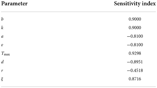
Table 1. Sensitivity indexes of R0 to model parameters.
Numerical simulation
In this section, a simulation is carried out to prove the accuracy of the aforementioned theoretical analysis.
Algorithm
Before the simulation, first, we provide the algorithm to solve the fractional-order differential equation (35, 36):
where Tsim is time length, k = 1, 2, 3, ..., N, N = [Tsim/h], m = [τ/h], and x(0) = x0, v(0) = v0, w(0) = w0, y(t) = y0, z(t) = z0, t ∈ [−τ, 0] are the initial conditions. .
Simulation of asymptotically stable infection-free equilibrium
First, we simulate the case of infection-free. The parameters are shown in Table 2.
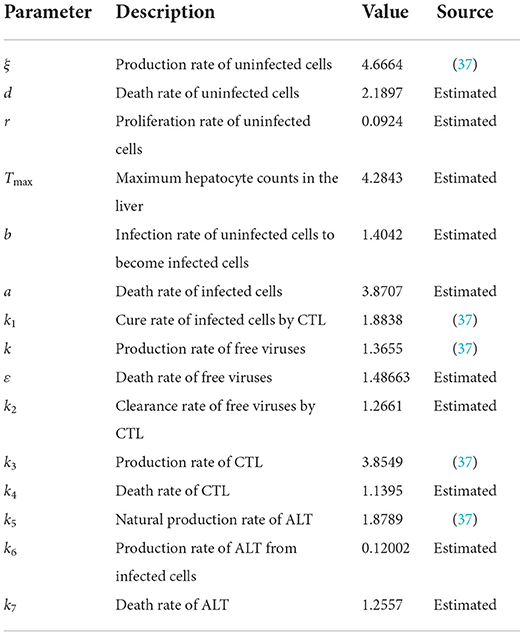
Table 2. Description of parameters and values when R0 < 1.
The time length is 400, and the initial conditions are x(0) = 1, v(0) = 1, w(0) = 1, y(t) = 1, z(t) = 1, t ∈ [−τ, 0]. The order α = 0.9 and the time delay τ = 0.7. Therefore, we have E0 = (x0, y0, v0, z0, w0) = (2.0289, 0, 0, 0, 1.4372), and the basic reproduction number R0 = 0.7546.
The behaviors of the uninfected cells (x), infected cells (y), free viruses (v), CTLs (z), and ALT (w) are shown in Figure 1. In Figure 1, all individuals converge to the infection-free equilibrium E0, and the basic reproduction number R0 is 0.7546, which is smaller than 1. This coincides with our theoretical analysis, which showed that when R0 < 1, the infection-free equilibrium E0 is asymptotically stable.
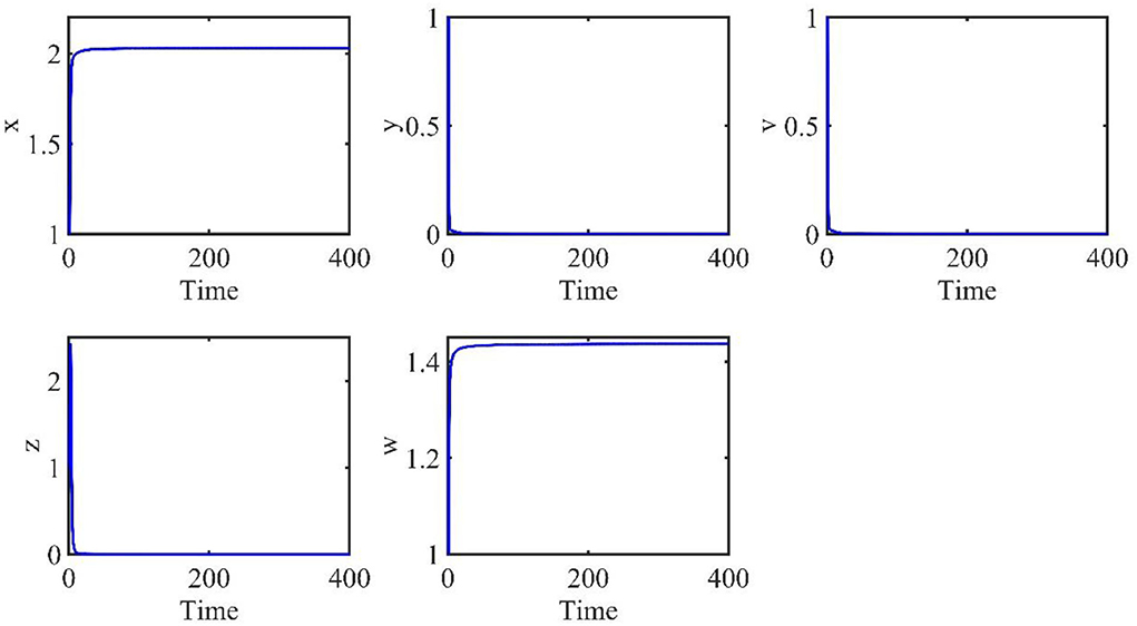
Figure 1. Dynamic change trend of uninfected cells (x), infected cells (y), free viruses (v), CTLs (z), and ALT (w) with R0 < 1 and τ = 0.7.
Simulation of asymptotically stable infection equilibrium
The theoretical analysis of the infection equilibrium is verified in this section. Similarly, the parameters are shown in Table 3.
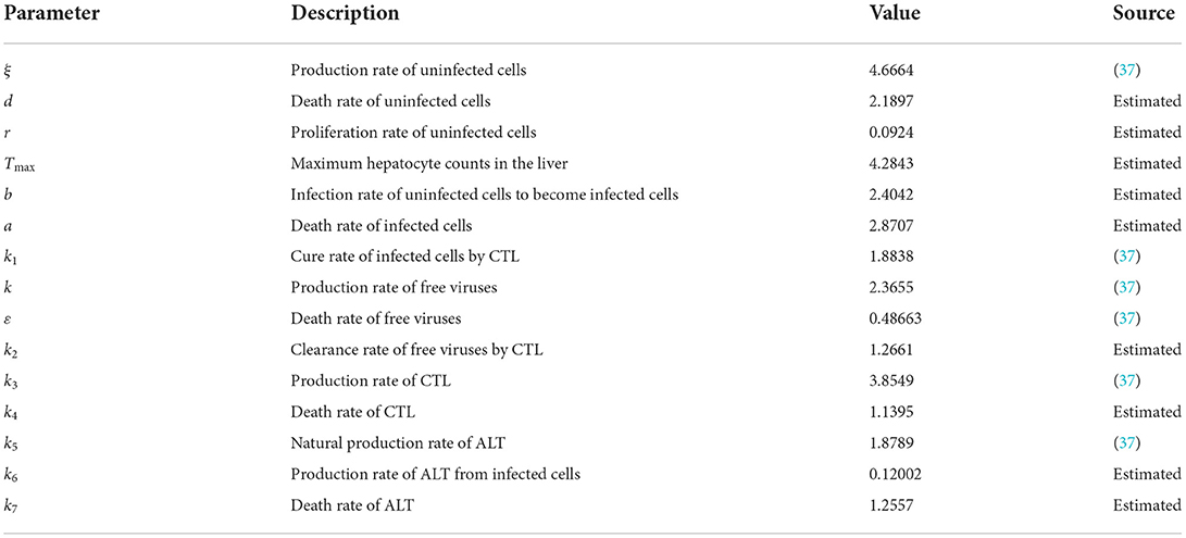
Table 3. Description of parameters and values when R1 > 1.
The initial conditions are the same as in the previous section. The time length is 400. The order α = 0.9, and the time delay τ = 1.2. Therefore, the infection equilibrium is as follows: E1 = (x1, y1, v1, z1, w1) = (1.2762, 0.3341, 0.5338, 1.0787, 1.4802), and the basic reproduction number is R1 = 2.0132.
Figure 2 is the behavior of the uninfected cells (x), infected cells (y), free viruses (v), CTLs (z), and ALT (w) with R1 > 1 and τ = 1.2. From Figure 2, we know that although all the individuals oscillate at the beginning, they converge to infection equilibrium E1shortly. Figure 3 shows the phase portraits of the uninfected cell–infected cell–free virus space; the arrow indicates the direction of convergence of the phase portraits, and it converges to the infection equilibrium E1 (red dot).
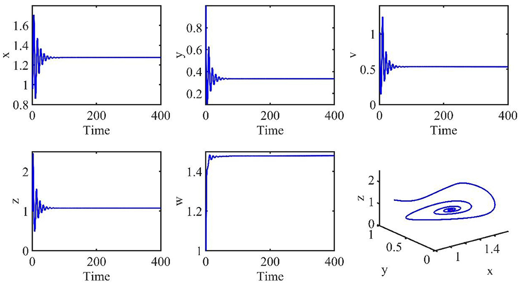
Figure 2. Dynamic change trend of uninfected cells (x), infected cells (y), free viruses (v), CTLs (z), ALT (w), and phase portraits of the xyz-space with R1 > 1 and τ = 1.2.
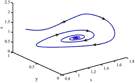
Figure 3. Phase portraits of the xyz-space with R1 > 1 and τ = 1.2.
Simulation of the Hopf bifurcation of the infection equilibrium
In this subsection, the Hopf bifurcation of the infection equilibrium is simulated. All parameters are the same as those in Section Simulation of asymptotically stable infection equilibrium, except τ = 3.2.
Figure 4 shows that when τ = 3.2, the uninfected cells (x), infected cells (y), free viruses (v), CTLs (z), and ALT (w) oscillate periodically around the infection equilibrium E1. Figure 5 shows the phase portraits of the uninfected cell–infected cell–free virus space, and when τ = 3.2, the phase portraits are a stable limit cycle which is around the infection equilibrium E1. The bifurcation diagram (Figure 6) shows that the stability of infection equilibrium E1 changes at τ = 1.2.
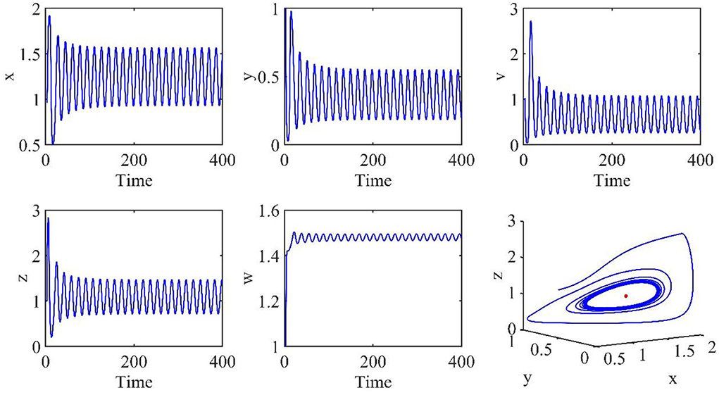
Figure 4. Dynamic change trend of uninfected cells (x), infected cells (y), free viruses (v), CTLs (z), ALT (w), and phase portraits of the xyz-space with τ = 3.2.
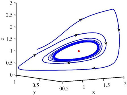
Figure 5. Phase portraits of the xyz-space with τ = 3.2.
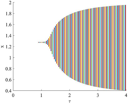
Figure 6. One parameter bifurcation diagram with respect to τ.
Simulation of phase portraits with different orders
In this section, the phase portraits with different orders are studied by using the method of numerical simulation. The initial order is α = 0.75, and with step of 0.05, the order increases to 0.99. The phase portraits also used the uninfected cell–infected cell–free virus space. As shown in Figure 7, when τ = 1.2 and the order (α) increases from 0.75 to 0.99, the volume of the phase portraits becomes bigger and the phase portraits become more complicated. Furthermore, the numerical simulations indicated that when the order increases from 0.75 to 0.95, the uninfected cell–infected cell–free virus space converges to the infection equilibrium E1. However, when α = 0.99, the phase portrait is a stable limit cycle, which is around the infection equilibrium E1. This indicated that the order can significantly affect the stability of the system.
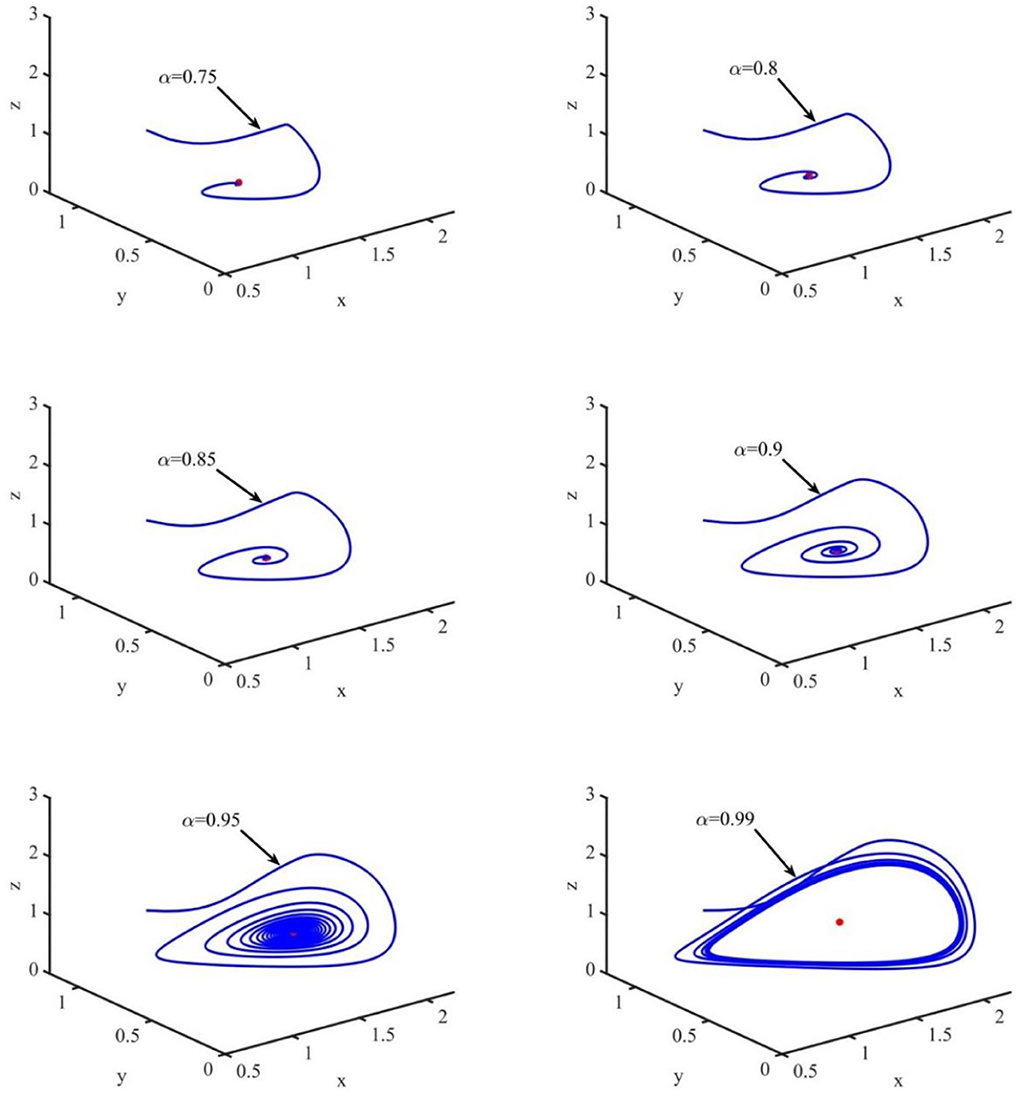
Figure 7. Phase portraits of the xyz-space with τ = 1.2 and α = 0.75, α = 0.80, α = 0.85, α = 0.90, and α = 0.99.
Conclusion and discussion
In this study, a fractional differential model of HBV infection with time delay and logistic proliferation was proposed in order to better understand the infection mechanism and realize the infection progression. First, the infection-free equilibrium, infection equilibrium, and the basic reproduction number were computed. In epidemiology, R0 is considered the most important parameter, which provides an insight into how the disease spreads and helps us understand how to control the disease. Therefore, we proved that if the basic reproduction number , the infection-free equilibrium (E0) is locally asymptotically stable, which indicated that if the basic reproduction number R0 < 1 can be controlled in patients, hepatitis B will disappear. Similarly, the stability analysis of the infection-free equilibrium (E1) was discussed. In addition, the Hopf bifurcation of the infection equilibrium was studied at the theoretical level. Furthermore, sensitivity was analyzed to screen out the parameters that can significantly affect the basic reproduction number in our model. The results indicated that decreasing the infection rate (b), production rate of free viruses (k) and production rate of uninfected cells (ξ) can significantly decrease the basic reproduction number (R0). Similarly, increasing the death rate of infected cells (a), the death rate of free viruses (ε) and he death rate of uninfected cells (d) can also decrease the basic reproduction number (R0). Therefore, in order to keep R0 < 1, the patient can decrease parameters b, k, and ξ or increase a, ε, and d to achieve the purpose of treatment.
In order to verify the accuracy of the aforementioned theoretical analysis, the numerical simulations were carried out. The simulation results showed that when R0 < 1 and τ < 1.2, the infection-free equilibrium E0 is asymptotically stable, which indicates that the disease will disappear. When R1 > 1 and τ < 1.2, the infection equilibrium E1 is asymptotically stable, which indicates that the disease could be mitigated and will lead to a lower infectious class over a period. However, with the increase in τ, the uninfected cells, infected cells, free viruses, CTL levels, and ALT levels oscillate periodically around the infection equilibrium E1, and the phase portrait is a stable limit cycle, which around the infection equilibrium E1 indicate that the disease would be out of control. Furthermore, the simulations also indicated that the order can significantly affect the stability of the system. For example, if the order is in the range of 0.75–0.95, the phase portraits converge to the infection equilibrium E1, and when α = 0.99, the phase portrait is a stable limit cycle.
Therefore, time delay and fractional order are necessary factors that should be considered in modeling HBV infection and for researching dynamic characteristics. Although the process of HBV infection is more complicated than is established in this study, we believe that the model and analysis can play an important role in improving the HBV treatment regimen.
Data availability statement
The original contributions presented in the study are included in the article/supplementary material, further inquiries can be directed to the corresponding authors.
Author contributions
DS: conceptualization, methodology, software, and writing—reviewing and editing. JL: software, methodology, and writing. XS: supervision, writing—review editing. GP: writing—review editing. All authors contributed to the article and approved the submitted version.
Funding
The work is supported by The National Natural Science Foundation of China (62103287 and 62003071), Basic Research General Project of Shenzhen (JCYJ20210324103209026), PhD Basic Research Initiation Project (RCBS20200714114856171), and Clinical Research Project of Shenzhen Second People's Hospital (20213357007).
Conflict of interest
The authors declare that the research was conducted in the absence of any commercial or financial relationships that could be construed as a potential conflict of interest.
Publisher's note
All claims expressed in this article are solely those of the authors and do not necessarily represent those of their affiliated organizations, or those of the publisher, the editors and the reviewers. Any product that may be evaluated in this article, or claim that may be made by its manufacturer, is not guaranteed or endorsed by the publisher.
References
1. WHO. Hepatitis B. (2021). Available online at: https://www.who.int/news-room/fact-sheets/detail/hepatitis-b (accessed June 24, 2022).
2. Li M, Zu J. The review of differential equation models of HBV infection dynamics. J Virol Methods. (2019) 266:103–13. doi: 10.1016/j.jviromet.2019.01.014
3. James Peter O, Ojo MM, Viriyapong R, Abiodun Oguntolu F. Mathematical model of measles transmission dynamics using real data from Nigeria. J Diff Equ Appl. (2022) 28:753–70. doi: 10.1080/10236198.2022.2079411
4. Peter OJ, Qureshi S, Yusuf A, Al-Shomrani M, Idowu AA. A new mathematical model of COVID-19 using real data from Pakistan. Result Phys. (2021) 24:104098. doi: 10.1016/j.rinp.2021.104098
5. Ojo MM, Peter OJ, Goufo EFD, Panigoro HS, Oguntolu FA. Mathematical model for control of tuberculosis epidemiology. J Appl Math Comput. (2022). doi: 10.1007/s12190-022-01734-x
6. Elaiw AM, AlShamrani NH. Global stability of humoral immunity virus dynamics models with nonlinear infection rate and removal. Nonlinear Anal Real World Appl. (2015) 26:161–90. doi: 10.1016/j.nonrwa.2015.05.007
7. Nowak MA, BS, Hill AM. Viral dynamics in hepatitis B virus infection. Proc Natl Acad Sci U S A. (1996) 93:4398–402. doi: 10.1073/pnas.93.9.4398
8. Su Y, Sun D, Zhao L. Global analysis of a humoral and cellular immunity virus dynamics model with the Beddington–DeAngelis incidence rate. Math Methods Appl Sci. (2015) 38:2984–93. doi: 10.1002/mma.3274
9. Manna K, Chakrabarty SP. Chronic hepatitis B infection and HBV DNA-containing capsids: modeling and analysis. Commun Nonlinear Sci Numer Simul. (2015) 22:383–95. doi: 10.1016/j.cnsns.2014.08.036
10. Li J, Wang K, Yang Y. Dynamical behaviors of an HBV infection model with logistic hepatocyte growth. Math Comput Model. (2011) 54:704–11. doi: 10.1016/j.mcm.2011.03.013
11. Prakash M, Balasubramaniam P. Bifurcation analysis of macrophages infection model with delayed immune response. Commun Nonlinear Sci Numer Simul. (2016) 35:1–16. doi: 10.1016/j.cnsns.2015.10.012
12. Sun C, Cao Z, Lin Y. Analysis of stability and Hopf bifurcation for a viral infectious model with delay. Chaos, Soliton, and Fractals. (2007) 33:234–45. doi: 10.1016/j.chaos.2005.12.029
13. Zhang Z, Kundu S, Tripathi JP, Bugalia S. Stability and Hopf bifurcation analysis of an SVEIR epidemic model with vaccination and multiple time delays. Chaos, Solitons, and Fractals. (2020) 131:109483. doi: 10.1016/j.chaos.2019.109483
14. Babasola O, Oshinubi K, Peter OJ, Onwuegbuche FC, Khan I. Time-delayed modelling of the COVID-19 dynamics with a convex incidence rate. Res Sq. (2022). doi: 10.21203/rs.3.rs-1814397/v1
15. Chinnathambi R, Rihan FA. Stability of fractional-order prey–predator system with time-delay and Monod–Haldane functional response. Nonlinear Dyn. (2018) 92:1637–48. doi: 10.1007/s11071-018-4151-z
16. Sun D, Lu L, Liu F, Duan L, Wang D, Xiong J. Analysis of an improved fractional-order model of boundary formation in the Drosophila large intestine dependent on Delta–Notch pathway. Adv Differ Equ. (2020) 2020:377. doi: 10.1186/s13662-020-02836-1
17. Mondal S, Lahiri A, Bairagi N. Analysis of a fractional order eco-epidemiological model with prey infection and type 2 functional response. Math Methods Appl Sci. (2017) 40:6776–89. doi: 10.1002/mma.4490
18. Almeida R. Analysis of a fractional SEIR model with treatment. Appl Math Lett. (2018) 84:56–62. doi: 10.1016/j.aml.2018.04.015
19. George Maria Selvam A, Abraham Vianny D. Bifurcation and dynamical behaviour of a fractional order Lorenz-Chen-Lu like chaotic system with discretization. J Phys Conf Ser. (2019) 1377:012002. doi: 10.1088/1742-6596/1377/1/012002
20. Wang X, Wang Z, Huang X, Li Y. Dynamic analysis of a delayed fractional-order SIR model with saturated incidence and treatment functions. Int J Bifurc Chaos. (2019) 28:1850180. doi: 10.1142/S0218127418501808
21. Li H, Huang C, Li T. Dynamic complexity of a fractional-order predator–prey system with double delays. Phys A Stat Mech Appl. (2019) 526:120852. doi: 10.1016/j.physa.2019.04.088
22. Balci E, Öztürk I, Kartal S. Dynamical behaviour of fractional order tumor model with Caputo and conformable fractional derivative. Chaos, Solitons, and Fractals. (2019) 123:43–51. doi: 10.1016/j.chaos.2019.03.032
23. Ye Y, Kou C. Stability analysis for a fractional HIV-1 model with time delay. In 4th International Conference on Biomedical Engineering and Informatics. IEEE, New York, NY (2011).
24. Nwajeri UK, Fadugba D, Ohaeri EO, Oshinubi K, Ogunrinde RR, Ogunrinde PB. Co-Dynamic Model of Drug Trafficking and Money Laundering Coupled with Atangana-Baleanu Derivative. (2022). doi: 10.2139/ssrn.4165832
25. Peter OJ. Transmission Dynamics of Fractional Order Brucellosis Model Using Caputo–Fabrizio Operator. Int. J. Diff. Equ. (2020) 2020:2791380. doi: 10.1155/2020/2791380
26. Peter OJ, Shaikh AS, Ibrahim MO, Nisar KS, Baleanu D, Khan I, et al. Analysis and dynamics of fractional order mathematical model of COVID-19 in Nigeria using Atangana–Baleanu operator. Comput Mater Contin. (2021) 66:1823–48. doi: 10.32604/cmc.2020.012314
27. Ogunrinde RB, Nwajeri UK, Fadugba SE, Ogunrinde RR, Oshinubi KI. Dynamic model of COVID-19 and citizens reaction using fractional derivative. Alex Eng J. (2021) 60:2001–12. doi: 10.1016/j.aej.2020.09.016
28. Peter OJ, Yusuf A, Oshinubi K, Oguntolu FA, Lawal JO, Abioye AI, et al. Fractional order of pneumococcal pneumonia infection model with Caputo Fabrizio operator. Result Phys. (2021) 29:104581. doi: 10.1016/j.rinp.2021.104581
29. Diethelm K, A. fractional calculus based model for the simulation of an outbreak of dengue fever. Nonlinear Dyn. (2012) 71:613–9. doi: 10.1007/s11071-012-0475-2
30. González-Parra G, Arenas AJ, Chen-Charpentier BM. A fractional order epidemic model for the simulation of outbreaks of influenza A(H1N1). Math Methods Appl Sci. (2014) 37:2218–26. doi: 10.1002/mma.2968
31. Danane J, Allali K, Hammouch Z. Mathematical analysis of a fractional differential model of HBV infection with antibody immune response. Chaos, Solitons, and Fractals. (2020) 136:109787. doi: 10.1016/j.chaos.2020.109787
32. Gao F, Li X, Li W, Zhou X. Stability analysis of a fractional-order novel hepatitis B virus model with immune delay based on Caputo–Fabrizio derivative. Chaos, Solitons, and Fractals. (2021) 142:110436. doi: 10.1016/j.chaos.2020.110436
33. Simelane SM, Dlamini PG, A. fractional order differential equation model for Hepatitis B virus with saturated incidence. Result Phys. (2021) 24:104114. doi: 10.1016/j.rinp.2021.104114
34. Su Y, Sun D. Optimal control of anti-HBV treatment based on combination of traditional Chinese medicine and western medicine. Biomed Signal Process Control. (2015) 15:41–8. doi: 10.1016/j.bspc.2014.09.007
35. Adebisi AF, Ojurongbe TA, Okunlola KA, Peter OJ. Application of Chebyshev polynomial basis function on the solution of Volterra integro-differential equations using Galerkin method. Math Comput Sci. (2021) 2:41–51. doi: 10.30511/mcs.2021.540133.1047
36. Christie I, Adebayo T, Peter O, Folasade A. Numerical solution of two-dimensional Fredholm integro-differential equations by Chebyshev integral operational matrix method. J Appl Math Comput Mech. (2022) 21:29–40. doi: 10.17512/jamcm.2022.1.03
Keywords: HBV model, time delay, fractional order, stability, Hopf bifurcation
Citation: Sun D, Liu J, Su X and Pei G (2022) Fractional differential equation modeling of the HBV infection with time delay and logistic proliferation. Front. Public Health 10:1036901. doi: 10.3389/fpubh.2022.1036901
Received: 05 September 2022; Accepted: 27 September 2022;
Published: 11 November 2022.
Edited by:
Olumide Babatope Longe, Academic City University College, GhanaReviewed by:
Kayode Oshinubi, Université Grenoble Alpes, FranceOlumuyiwa James Peter, University of Medical Sciences, Nigeria
Olalekan Lekings Abdulrasheed Ogunjimi, Trinity University Lagos, Nigeria
Copyright © 2022 Sun, Liu, Su and Pei. This is an open-access article distributed under the terms of the Creative Commons Attribution License (CC BY). The use, distribution or reproduction in other forums is permitted, provided the original author(s) and the copyright owner(s) are credited and that the original publication in this journal is cited, in accordance with accepted academic practice. No use, distribution or reproduction is permitted which does not comply with these terms.
*Correspondence: Deshun Sun, c3VuX2Rlc2h1bkBoaXQuZWR1LmNu; Guoxian Pei, cGVpZ3hAc3VzdGVjaC5lZHUuY24=
†These authors have contributed equally to this work