Tracking Ideal Varieties and Cropping Techniques for Agroecological Weed Management: A Simulation-Based Study on Pea

Pea or Pisum sativum L. is a key diversification crop, but current varieties are not very competitive against weeds. The objective was to identify, depending on the type of cropping system and weed flora, (1) the key pea parameters that drive crop production, weed control and weed contribution to biodiversity, (2) optimal combinations of pea-parameter values and crop-management techniques to maximize these goals. For this, virtual experiments were run, using FLORSYS, a mechanistic simulation model. This individual-based 3D model simulates daily crop-weed seed and plant dynamics over the years, from the cropping system and pedoclimate. Here, this model was parameterized for seven pea varieties, from experiments and literature. Moreover, ten virtual varieties were created by randomly combining variety-parameter values according to a Latin Hypercube Sampling (LHS) plan, respecting parameter ranges and correlations observed in the actual varieties. A global sensitivity analysis was run, using another LHS plan to combine pea varieties, crop rotations and management techniques in nine contrasting situations (e.g., conventional vs. organic, no-till, type of weed flora). Simulated data were analyzed with classification and regression trees (CART). We highlighted (1) Parameters that drive potential yield and competitivity against weeds (notably the ability to increase plant height and leaf area in shaded situations), depending on variety type (spring vs. winter) and cropping system. These are pointers for breeding varieties to regulate weeds by biological interactions; (2) Rules to guide farmers to choose the best pea variety, depending on the production goal and the cropping system; (3) The trade-off between increasing yield potential and minimizing yield losses due to weeds when choosing pea variety and management, especially in winter peas. The main pea-variety rules were the same for all performance goals, management strategies, and analyses scales, but further rules were useful for individual goals, strategies, and scales. Some variety features only fitted to particular systems (e.g., delayed pea emergence is only beneficial in case of herbicide-spraying and disastrous in unsprayed systems). Fewer variety rules should be compensated by more management rules. If one of the two main weed-control levers, herbicide or tillage, was eliminated, further pea-variety and/or management rules were needed.

Introduction

Today, pea (Pisum sativum L.) is a minor crop in temperate arable cropping systems (e.g., for France¹). However, integrating pea into rotations potentially has many benefits. As a legume crop, it allows reducing nitrogen fertilizer use (Nemecek et al., 2008) and diversifying cereal-based rotations to control weed infestations (Chauvel et al., 2001) or pests (Ratnadass et al., 2012). Pea also provides proteins for both human and animal food supply (Voisin et al., 2014; Duc et al., 2015; Watson et al., 2017).

Pea reduces weed infestation at the rotation scale by diversifying weed control options and disrupting the growing season of the more harmfula utumn-emerging weeds (Chauvel et al., 2001). These effects are essential in the necessary shift from herbicide-based to agroecological weed management (Weisberger et al., 2019). However, the current pea varieties are not very competitive against weeds, notably because of a slow crop establishment (McDonald, 2003). Pea is known to be genetically diverse, in terms of flowering precocity, soil cover, plant height, and architecture (Espósito et al., 2007; Vocanson and Jeuffroy, 2008; Burstin et al., 2015; Spies et al., 2017), and collections of pea lines are available (Smýkal et al., 2012; Tayeh et al., 2015; Siol et al., 2017). Potentially, more competitive varieties could be produced. But, though the traits that make a crop competitive against weeds are known in general (Colbach et al., 2019) and, particularly for cereals (maize, Ford and Pleasant, 1994; barley, Christensen, 1995; Mennan and Zandstra, 2005; wheat, Drews et al., 2009; rice, Mahajan et al., 2014), they are not yet known specifically for pea. These studies highlighted the key role of shade response, which is not among the traits routinely monitored during crop selection.

Screening existing pea lines in experiments is not only time-consuming but presents methodological drawbacks when it comes to assessing weed harmfulness. It is notoriously difficult to correctly estimate crop yield loss due to weeds because it is next to impossible to ensure a continuously weed-free control to measure potential yield (Colbach et al., 2020c). Many studies thus use weed biomass (or worse, weed densities) as a proxy for yield loss (see references in Colbach et al., 2020c) but the results are often difficult to extrapolate to other situations. Indeed, competitive crop traits were shown to vary in terms of impact between years, because of weather or management effects (see references in Andrew et al., 2015).

Working with mechanistic (process-based) models makes it easier to identify limiting factors and relevant species traits. Consequently, many studies now rely on simulation to assess crop genotypes or to identify ideotypes (i.e., theoretical ideal crop plants that combine traits to optimize crop performance in a particular environment, crop management and end-use, Martre et al., 2015), whether for, e.g., tolerance to climate change (Tao et al., 2017), fruit quality (Memmah et al., 2014) or for weed management (Bastiaans et al., 1997; Colbach et al., 2019). One of the rare pea studies (Jeuffroy et al., 2012) compared contrasting pea varieties (including virtual ones based on expert knowledge), evaluating their performance in response to soil compaction in interaction with tillage/sowing dates and weather. However, their objective was to assess the robustness of genotypes and management strategies relative to weather repetitions rather than to identify key parameters or optimal parameter-value combinations.

The quality of these various assessments is highly dependent on the model type and its prediction quality. When focusing on pea competitivity against weeds, we need models that produce realistic predictions of crop-weed interactions in a large range of cropping systems, pedoclimates, and weed floras. This means an individual-based model to account for the temporal and morphological plasticity in weeds (Renton, 2013; Colbach et al., 2021). It should be parameterized for many crop and weed species to account for the diverse weed floras in arable crops (Fried et al., 2008). It must include all crop management techniques to account for both direct and indirect (e.g., via impacts on the environment) effects on weeds (Colbach and Debaeke, 1998; Colbach et al., 2021), and this over several years or decades to account for weed seed persistence in the soil (Lewis, 1973). To date, FLORSYS (Colbach et al., 2021) is the model that best meets these needs.

The objective of the present study was to identify parameters that make pea competitive against weeds, depending on management strategies. To achieve this, we (1) parameterized the FLORSYS model with contrasting pea varieties from experiments and literature, (2) created virtual varieties based on these data, (3) ran virtual experiments with these actual and virtual varieties in contrasting cropping systems to identify the pea parameters that drive crop production, weed disservices and services (hence (dis)services), (4) identified optimal pea-parameter value combinations, depending on the production goal and the cropping-system type. Production goals included not only yield, but also reduced herbicide use and weed contribution to biodiversity.

Materials and Methods

The Virtual Field FLORSYS

FLORSYS is a virtual field on which cropping systems can be experimented with a large range of virtual measurements of crop, weed, and environmental state variables (Gardarin et al., 2012; Munier-Jolain et al., 2013, 2014; Colbach et al., 2014a,b, 2021; Pointurier et al., 2021).

Weed and Crop Life Cycle

The input variables of FLORSYS consist of (1) a description of the simulated field (daily weather, latitude, and soil characteristics); (2) all the crops and management operations in the field, with dates, tools, and options; and (3) the initial weed seed bank. These input variables influence the annual life cycle of annual weeds and crops, with a daily time-step.

Pre-emergence stages (surviving, dormant, and germinating seeds, emerging seedlings) are driven by seed depth, soil structure, temperature, and water potential. The crop-weed canopy is represented in 3D, with each crop and weed plant schematized as a cylinder (above ground) and on top of a spilled cone (below ground). Post-emergence processes (e.g., photosynthesis, respiration, growth, shade response) are driven by light availability and air temperature. At plant maturity, weed seeds are added to the soil seed bank; crop seeds are harvested to determine crop yield. Nitrogen stress is disregarded in the present model version, and water stress is only considered for pre-emergent processes.

The model is currently parameterized for 26 frequent and contrasting annual weed species and 32 crop species (section A.2 of the Supplementary Material).

Effect of Cultural Techniques

Life-cycle processes depend on the dates, options, and tools of management techniques (tillage, sowing, herbicides, mechanical weeding, mowing, harvesting), in interaction with weather and soil conditions on the day the operations are carried out (section A.3 of the Supplementary Material).

Indicators of Weed Impact on Crop Production and Biodiversity

FLORSYS simulates crop yield as well as indicators assessing weed impacts on crop production and biodiversity (Mézière et al., 2015; Colbach et al., 2020a) (see section A.4 of the Supplementary Material). Here, one yield indicator was considered, i.e., potential crop yield from weed-free simulations. Then, two indicators of weed harmfulness for crop production were analyzed: crop yield loss, as the relative crop yield difference of simulations with and without weeds, as well as field infestation. In addition, two indicators of weed contribution to biodiversity were included, i.e., weed species richness (illustrating wild plant biodiversity) and weed contribution to feeding domestic bees (as an example for functional biodiversity).

Domain of Validity

FLORSYS was evaluated with independent field data (Colbach et al., 2016; Pointurier et al., 2021). This showed that crop yields, daily weed species densities, and densities averaged over the years were generally well predicted and ranked as long as a corrective function was added to keep weeds from flowering during winter at more southern latitudes. Higher crop yield losses than those reported in previous field studies resulted from the simulation plan. This does not adapt practices to simulated weed floras and interannual weather variability (as farmers or trial managers would do), in order to discriminate the effect of crop species and management practices on weeds from the effect of weeds on the choice of crops and practices (Colbach and Cordeau, 2018).

Parameterize Contrasting Pea Varieties

Choosing Contrasting Pea Varieties and Necessary Experiments

For this study, seven pea varieties contrasting in terms of seasonality and morphology were chosen (Table 1A) and parameterized for FLORSYS. In FLORSYS, a crop species is represented by 220 parameters (section A.4 of the Supplementary Material). To parameterize pea varieties, we used existing literature (Lecomte et al., 2003; Raveneau et al., 2011; Tayeh et al., 2015; Castel et al., 2017; Varela Nicola, 2017; Colbach et al., 2020b), extracted parameters from other models (Brisson et al., 2009; Pointurier et al., 2021) and set up experiments when no parameter source was available. This was mainly the case for parameters describing potential plant morphology in unshaded conditions and response to shading by neighbor plants. These key processes drive crop-weed competition and determine how fast plants occupy space once they emerge, how much space they occupy, and how they adapt light capture when surrounded by neighbor plants. In FLORSYS, potential plant morphology in unshaded conditions depends on eight parameters per species and stage, for 11 plant stages (Figures 1A–H). Two further parameters determine maximum plant height and width in unlimiting growth conditions. These parameters determine plant dimensions, leaf area, and leaf-area distribution along plant height in unshaded conditions. Another five parameters per species and stage drive species response to shading, determining whether shaded plants invest more into plant height vs. width or into leaf vs. stem biomass, whether they reduce their leaf thickness to increase leaf area, and whether they shift their leaves upward or downward (Figures 1I–M).

TABLE 1

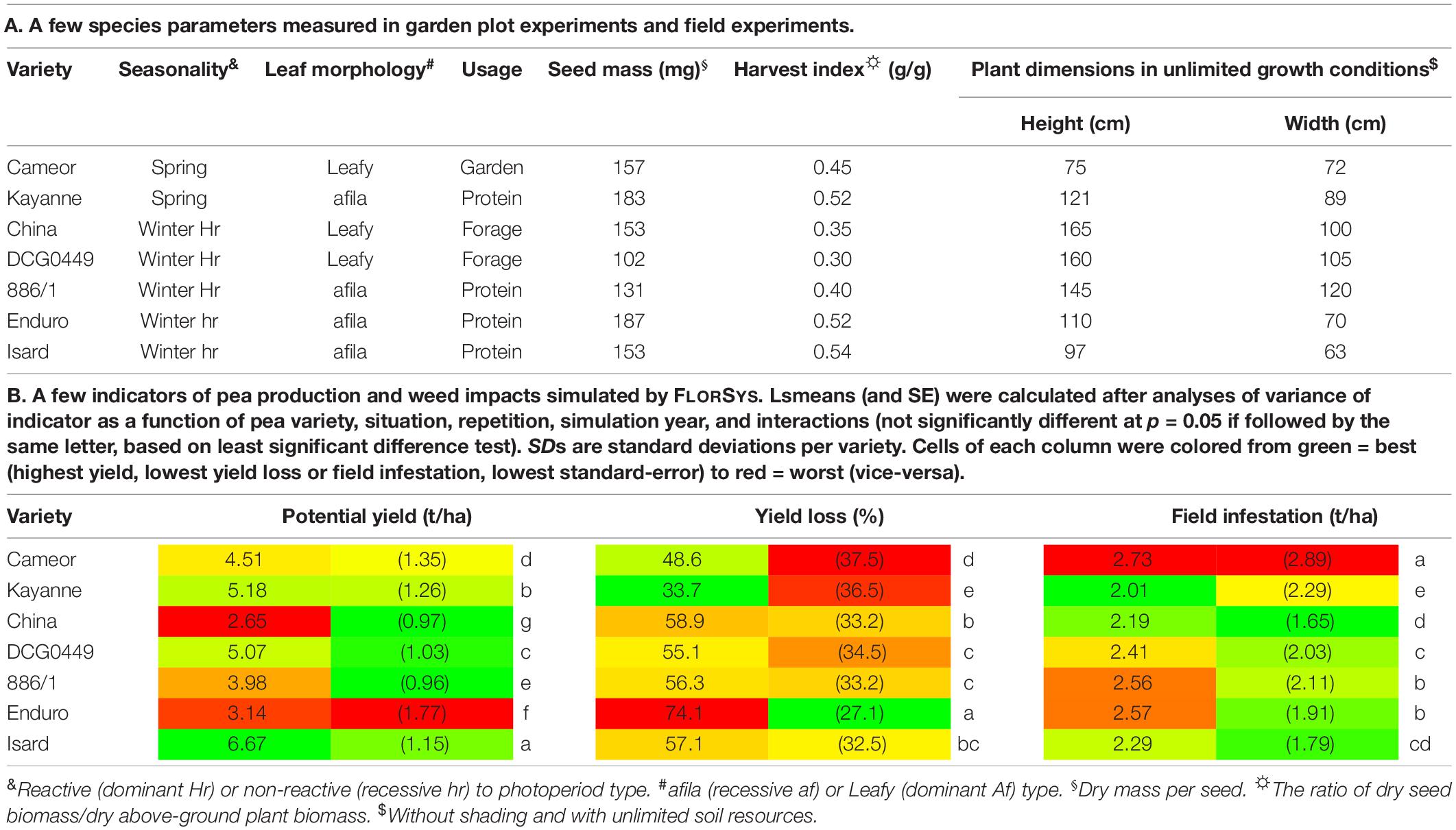
Table 1. List of pea (Pisum sativum L.) varieties tested in the present experiments.

FIGURE 1

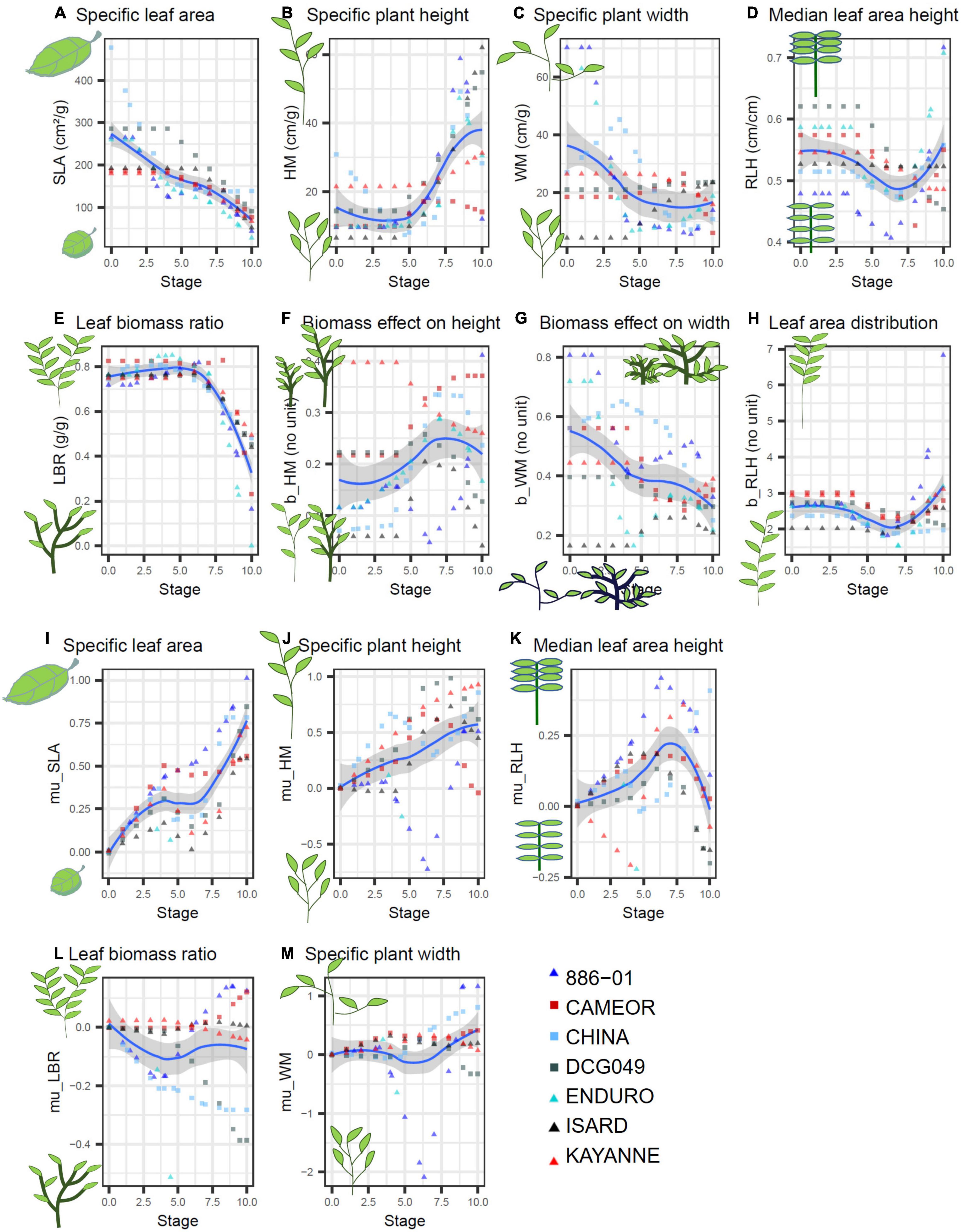
Figure 1. Parameters describing potential plant morphology in unshaded conditions (A–H) and shading response (I–M) measured on 7 pea varieties (red symbols = spring varieties, blueish colors = winter varieties, ▲ = afila, ■ = Leafy) over plant stages (BBCH) estimated from garden-plot experiments. SLA, plant leaf area/plant leaf biomass; LBR, plant leaf biomass/plant above-ground biomass; HM, plant height/plant above-ground biomass^b_HM; WM, plant width/plant above-ground biomass^b_WM; RLH, plant height below which 50% of leaf area are located/total plant height; b_RLH, shape parameter for leaf area distribution along plant height. mu_X shapes shade response of morphogical variable X (SLA, LBR, etc.) via X = X_unshaded ⋅ exp(-mu_X ⋅ shading intensity) (Colbach, 2020 ).

Garden Plot Experiments

The principle for estimating parameters of potential morphology and shading response in garden plots was described by Colbach et al. (2020b), based on the experimental and computational approaches developed by Munier-Jolain et al. (2014). In summary, isolated plants were sown in garden plots at the usual crop sowing dates, either under shading nets to mimic shading by neighbor plants or in unshaded conditions. The plants were placed at a distance exceeding 50 cm to avoid any interference. With each sampling date, plant-plant distance increased as more plants were taken out for measurements. Temperature and incident photosynthetically radiation (PAR) were measured continuously from sowing up to harvest inside and outside the shading cage. The plots were fertilized, watered, and hand-weeded regularly to avoid any water or nitrogen stress. Experiments were carried out in Dijon Burgundy, France (47°19′2.624″N, 5°4′26.883″E, 257 m asl), in 2010 (varieties 886/1, China, Enduro) and 2018 (varieties Cameor, DCG0449, Isard, Kayanne). The soil was 0.33 g/g clay, 0.49 g/g silt, and 0.17 g/g sand, with pH = 8.3 and 0.31 g organic matter/g soil.

For each variety, four to eight plants were sampled at five stages, ranging from the 2-leaf stage to the end of flowering. A vertical RGB image of each sampled plant was taken with a Canon powerShot SX20 IS (Canon Inc., Tokyo, Japan) commercial digital camera. For each image, a white calibration square (10 cm x 10 cm) was placed next to the plant to determine the spatial resolution of the camera. Vegetation was discriminated from the background using the excess green vegetation index (ExG) developed by Woebbecke et al. (1995). Then, binary thresholding (B&W) was performed using Otsu’s method (Otsu, 1979; Gée et al., 2021). Finally, the distribution of leaf area vs. relative plant height was determined. All the image-processing algorithms were implemented in Matlab (Version 2016b, The Mathworks, Natick, MA, United States).

Then, plant height and width, leaf area and biomass as well as total above-ground biomass were measured. For the latter two, leaves (including petioles), stems, and reproductive parts were discriminated. At each sampling stage and for each variety, these measurements were used to determine eight parameters (Figures 1A–H) characterizing potential plant morphology by fitting key state variables (e.g., plant height or width) against above-ground biomass using the plants grown in unshaded conditions. Then, five shade-response parameters (Figures 1I–M) were estimated by fitting the main morphology variables (e.g., specific leaf area SLA) against shading intensity (i.e., 1 – PAR in shaded/PAR in unshaded conditions) with a non-linear regression using all (shaded and unshaded) plants sampled at the same stage. Finally, for each variety, the parameter values from the five sampling stages were extrapolated to obtain parameter values for 11 BBCH stages ranging from emergence (stage 0) to full maturity (stage 10), using non-parametric regressions. All statistical analyses were carried out, using SAS (PROC REG, NLIN, and LOESS). Further details can be found in section B of the Supplementary Material.

Virtual Experiments

Create Virtual Pea Varieties

To determine correlations among pea parameters, Pearson correlations coefficients were calculated among the 220 parameters of the seven parameterized pea varieties, using corr() of Hmisc package of R (R Core Team, 2016). In addition, the minimum and maximum values for each quantitative parameter were determined for pea (section D.3 of the Supplementary Material). This range of variation was extended to [0.9 × min, 1.1 × max] for each parameter, but capped to remain biologically realistic (e.g., a proportion such as a harvest index needed to be in [0, 1] g/g).

Furthermore, ten virtual pea varieties were created by randomly drawing parameter values inside the extended range of variation of the seven actual varieties following a Latin Hypercube Sampling (LHS) plan and using the correlation matrix as constraints. This was done using the randomLHS() and LHScorcorr() functions of the lhs package of R.

Simulation Plan

The simulation plan aimed to evaluate the impact of pea parameters and management techniques in contrasting cropping systems, with a global sensitivity analysis (i.e., varying factors simultaneously to analyze the sensitivity to factors and their interactions, Saltelli et al., 2000). First, nine situations were chosen, varying in terms of rotation length and diversity, management techniques, and initial weed seed bank (Table 2). The two contrasting weed seed banks were based on a preliminary simulation study linking weed species to weed impact (section D.1 of the Supplementary Material).

TABLE 2

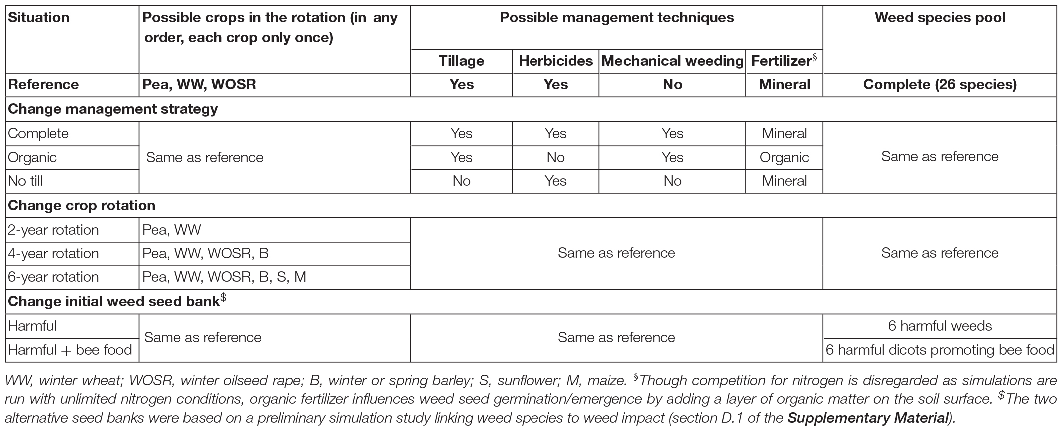
Table 2. Contrasting situations used to stratify the simulation plan testing the sensitivity of crop production and weed impact to pea parameters and management techniques with FLORSYS simulations. The two alternative weed seed banks were based on a preliminary simulation study linking weed species to weed impact (section D.1 of the Supplementary Material). For each situation, 400 cropping systems were built by randomly choosing management techniques based on a Latin Hypercube Sampling (LHS) plan and respecting the constraints of the situation. Pea varieties were chosen among a pool of 18 (virtual and actual) varieties.

For each situation, 400 cropping systems were built by randomly choosing management techniques based on a Latin Hypercube Sampling (LHS) plan and respecting the constraints of Table 2. For pea, varieties were chosen among a pool of 18 varieties: the seven actual varieties of Table 1, the ten virtual ones of section “Create Virtual Pea Varieties,” and a final one whose parameters were estimated from simulations with the STICS crop model (Brisson et al., 2003). Dates and options of techniques (e.g., depth, speed, and tool for tillage) were randomly chosen for each crop but respecting agronomic logic (e.g., winter wheat could not be sown in spring, sowing and harvesting dates of pea varieties allowed full maturation, no-tillage after crop sowing). The analysis of the Pearson correlations among simulation factors showed that our simulation plan was adequate to avoid confusing effects among management techniques. Indeed, the median correlation coefficient among crop management techniques as well as between techniques and rotation or situation varied from 0.05 to 0.09, depending on variety types and crops (details in section D.2.1 of the Supplementary Material). Pea parameters and management techniques were even less correlated (0.03–0.06). The Latin Hypercube Sampling (LHS) plan thus allowed decorrelating management variables. Correlations among rotation variables or between rotation and situation were much higher (0.12–0.21), reflecting the rotation rules fixed for each situation. Pea parameters were highly correlated (0.23–0.3), reflecting the biological correlations among variety characteristics, which we introduced by constraining the LHS via parameter correlations.

The 9 × 400 cropping systems were simulated over 12 consecutive years to assess long-term effects and repeated five times with five weather series consisting of randomly chosen records from the INRAE Dijon weather station (INRAE Climatik database). Each system × repetition was run twice, once starting with weeds and once without, to assess potential crop yield. Crop yield loss due to weeds was then calculated as (yield from weed-free simulation – yield from weedy simulation)/(yield from weed-free simulation). This simulation plan succeeded in producing differences in pea and weed (dis)services across situations (see details in section D.6 of the Supplementary Material).

Statistics

To make the indicators of potential crop yield and weed (dis)services (see section “Indicators of Weed Impact on Crop Production and Biodiversity”) comparable, they were rescaled to [0,1] with 0 corresponding to the worst value (lowest yield or biodiversity, highest harmfulness) across all situations, cropping systems, years and weather repetitions, and 1 to the best (highest yield or biodiversity, lowest harmfulness). To stress that a rescaled weed-harmfulness value of 1 means low harmfulness (e.g., low yield loss), we renamed such indicators as “weed-harmfulness control” (e.g., yield-loss control).

To analyze trade-offs among indicators of yield and weed (dis)services, a PCA was run across all situations with the PCA() function of R software version 4.0.1 (R Core Team, 2021), separately for cropping systems with spring vs. winter varieties.

To identify which simulation factors (situation, pea parameters, management techniques for peas and other crops, weather repetition) influence the indicators, classification and regression trees (CART) (Breiman et al., 1984) were run per pea variety type (spring or winter), either on annual data (years with a pea) or data averaged over the simulation, including years grown with crops other than a pea (rotation scale). The trees predict a continuous response variable (here either individual indicators, or a combination of several indicators hence called “performance profile”) from a set of discrete or continuous predictors (here situation, pea-variety parameters, crop management techniques). The data set is recursively split into two subsets along a threshold value of the predictor in order to maximize the difference between subsets (see example in Figure 2). Branches are combinations of predictor values that lead to predictions contained in leaf nodes. The trees were computed with the R package mvpart (Glenn De’ath, 2014). The optimal tree size was internally identified using a 10-fold cross-validation procedure to avoid overfitting. In the following, R² refers to the cross-validated R² of the resulting tree.

FIGURE 2

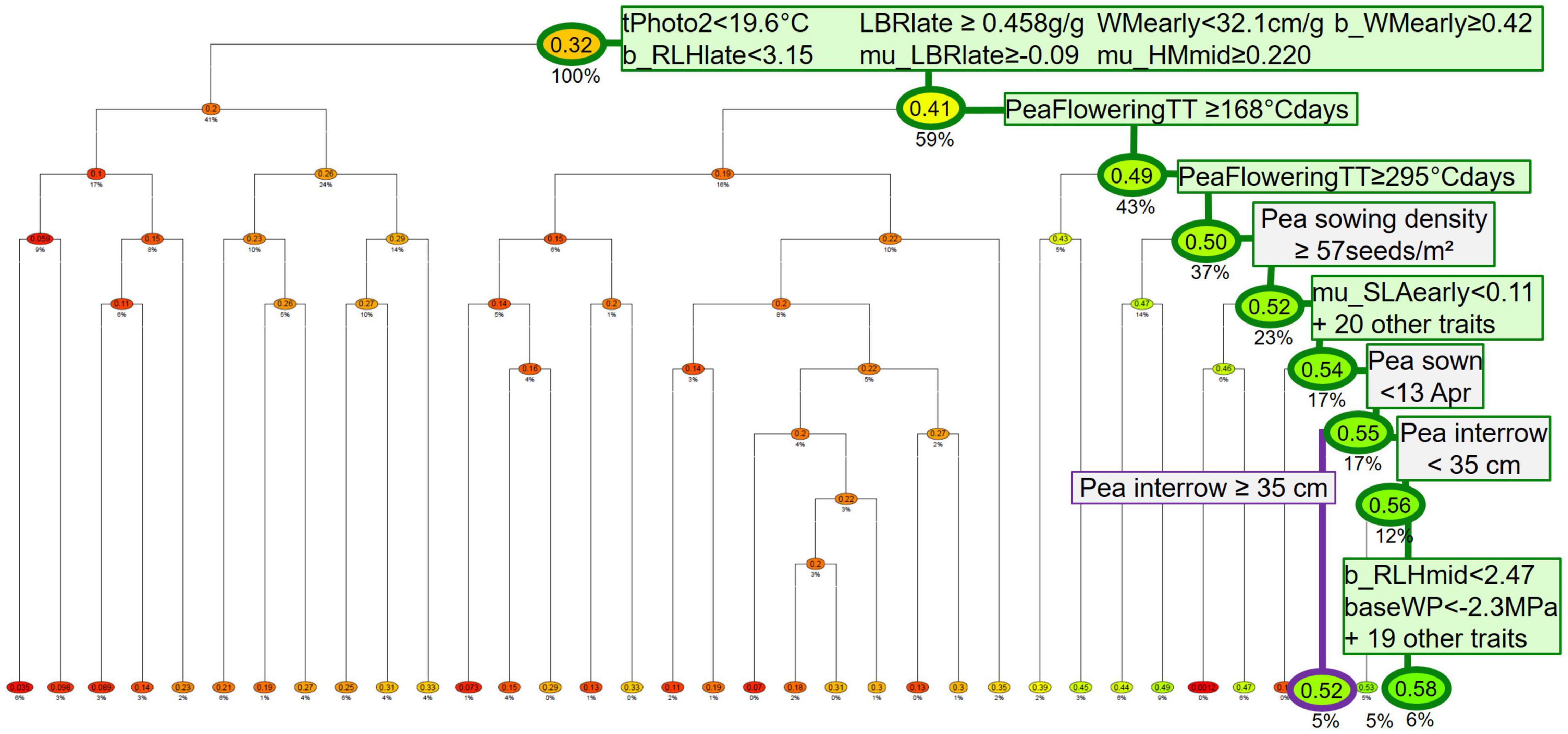
Figure 2. Example of regression and classification tree (CART) analyzing potential yield of spring pea from weed-free simulations (response variable) as a function of pea parameters (in green), pea management techniques, and other-crop techniques (in gray) (predictors). Only pea crops with herbicides were used here. The highlighted branches show the best and third-best performances (which are also shown in Table 5A). Boxes show principal and surrogate predictors and thresholds for splitting branches (only for the two highlighted branches). Leaves (at the bottom of the tree) and nodes show indicator values normed to [0 = lowest yield, 1 = highest yield of simulated data set]; leaves are colored from red (lowest yield) through yellow (intermeidate yield) to green (highest yield). Percentages below nodes show the proportion of individuals that fall into that node. The root node at the top of the tree has 100% since the dataset has not been split yet (Colbach, 2021 ).

TABLE 3

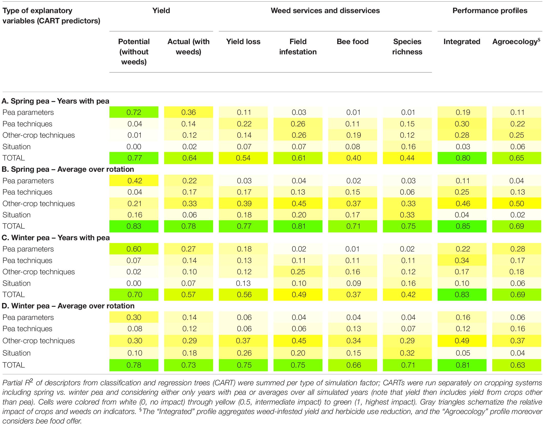
Table 3. Variability in weed (dis)service indicators is explained by the different types of simulation factors.

TABLE 4

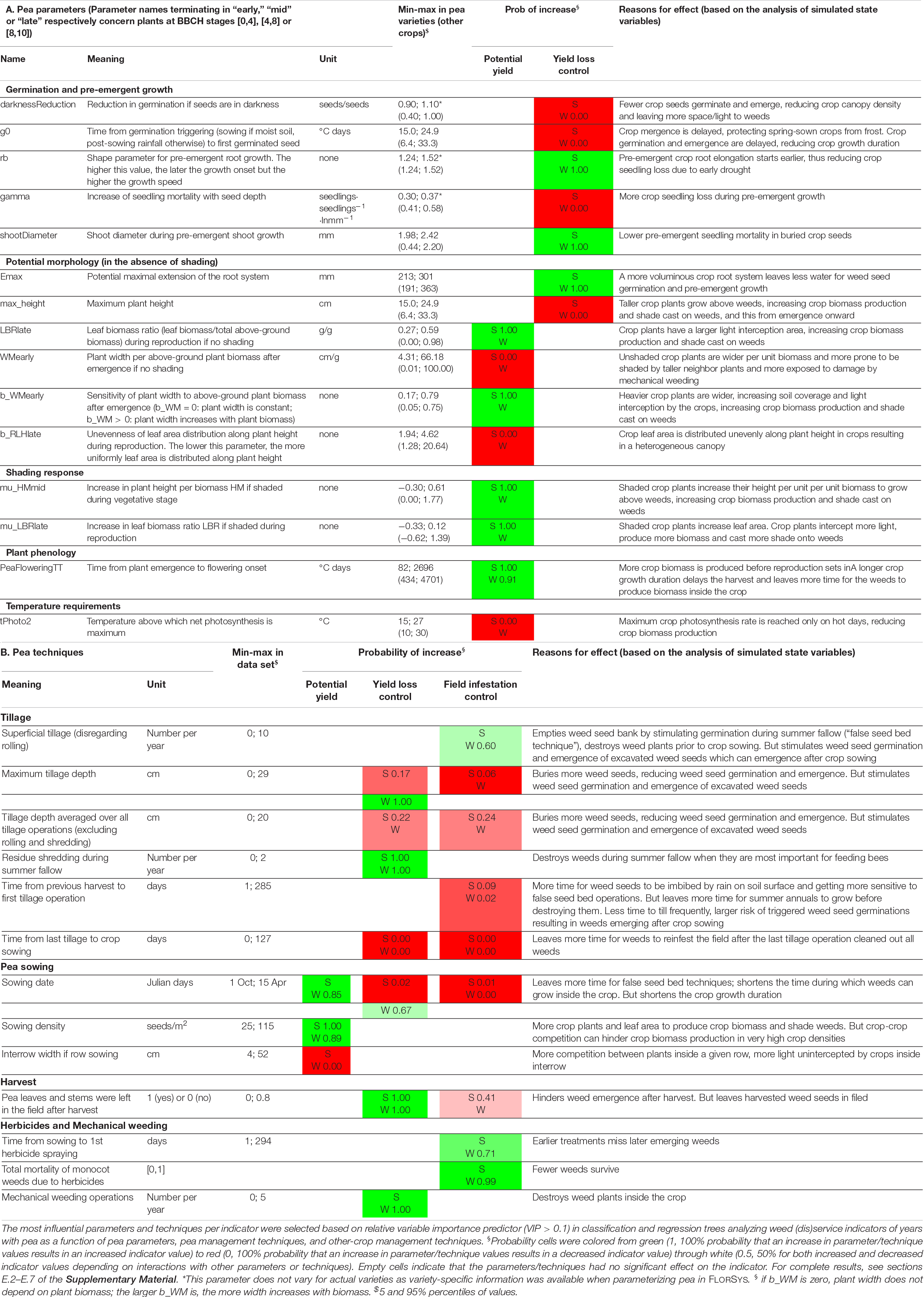
Table 4. The key pea parameters and techniques driving potential yield and yield loss due to weeds in Spring (S) and Winter (W) pea.

TABLE 5

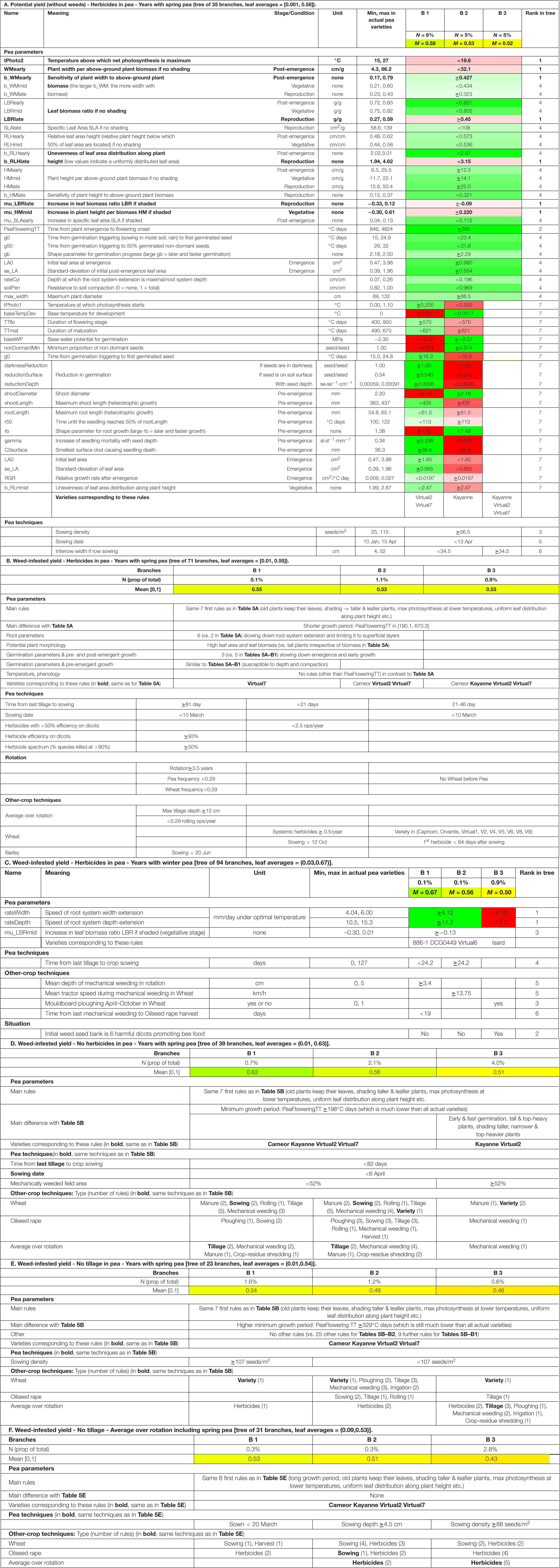
Table 5. Optimal combinations of pea parameters, pea management, and other-crop management, depending on the goal, situation, analysis scale, and pea variety type (complete results in section E.8 of the Supplementary Material). The three best scenarios (branches B1, B2, and B3) identified with classification and regression trees applied to 400 cropping systems × 12 years × 10 weather repetitions per situation. Indicator values were normed to [0, 1] with 0 the worst performance (i.e., lowest yield or highest yield loss) over all situations and 1 the best one (i.e., highest yield or lowest yield loss). In the case of multivariate response variables, branches were ordered by increasing values of the minimum of the response variables (see section “Statistics”). A and C: rules were colored from green (100% of the parameter range of variation of actual varieties consistent with the rule) to red (0% of the range covered) through white (50%).

Predictors (including surrogate variables that would split the data set exactly as the primary splitting variables) were ranked according to their relative Variable Importance Predictor (VIP, rescaled here by dividing by the total amount of variability explained by the tree, see section D.4 of the Supplementary Material). The CARTs were built, allowing up to “perfect” 20 surrogates (i.e., with raw agreement = 1) per split. In addition, the probability that the analyzed response variable increases when the predictor value increases were estimated by summing the relative number of individuals that split the branch toward a higher predictor value, over all tree nodes including the predictor as a primary or surrogate splitting variable. We defined the partial R² of a predictor as its relative VIP multiplied by the total R² of the tree. To assess the contribution of predictor classes (situation, pea parameters, pea techniques, other-crop techniques), partial R² was calculated for each class, summing partial R² over all predictors belonging to the class.

Finally, optimal combinations of pea parameter values and crop management techniques were identified for different performance goals, per variety type (spring or winter), analysis scale (years with pea or average over-rotation including all crops), and situation. Several individual performance goals were considered, maximizing either potential pea yield (i.e., yield in weed-free simulations), weed-infested pea yield (from weed-inclusive simulations), weed-based trophic resources for domestic bees, or weed species richness, or minimizing either crop yield loss due to weeds or field infestation. In addition, composite goals were included, called “Integrated” (maximizing weed-infested yield and minimizing herbicide use intensity), and “Agroecology” (the former plus maximizing bee-food offer). To identify these optimal combinations, CARTs were run per goal, variety type, and analysis scale (years with pea vs. average over-rotation). The three best branches were selected, i.e., those leading to the leaves with the highest indicator value (remember that, e.g., the lowest yield loss gives the highest rescaled indicator value). For multi-variate goals, the best branches were those with the highest minimum value of the constituting indicators. The best branch b of a given tree answers to the following condition:

$\underset{\mathrm{over}\mathrm{i}}{\min }\left({\text{T}}_{\text{bi}}\right)>\underset{\mathrm{over}{\mathrm{b}}^{\prime }}{\max }\left(\underset{\mathrm{over}\mathrm{i}}{\min }\left({\text{T}}_{{\mathrm{b}}^{\prime }\mathrm{i}}\right)\right)$

where T_bi is the value of the indicator i for branch b.

Here, only a few examples were presented, the complete results are in sections E and F of the Supplementary Material.

Results

Parameterizing Contrasting Pea Varieties

The garden-plot experiments allowed estimating the parameters related to potential plant morphology and shading response. These parameters were among those that the most discriminated the seven pea varieties (see section C.3 of the Supplementary Material). Differences between varieties depended on the analyzed parameter (Figure 1). There was, for instance, little difference among varieties for the leaf biomass ratio, i.e., the ratio of leaf biomass divided by aboveground plant biomass (Figure 1E). This ratio was around 0.8 until nearly flowering onset and then continuously decreased until full maturity, regardless of the variety. Other parameters differed according to the seasonal type, e.g., at early stages, specific leaf area (SLA, ratio of total leaf area divided by total leaf biomass) was lower for the two spring varieties (Cameor and Kayanne) tested here than for the five winter varieties (except Isard, Figure 1A). But, most parameters greatly varied among varieties, regardless of seasonal or morphological type (i.e., afila vs. leafy).

Trade-Offs Among Indicators of Pea Yield and Weed (Dis)services

Across the nine simulated situations, weed-infested pea yield (in the presence of weeds) was opposed to direct weed harmfulness for pea production (yield loss, harvest pollution by weed seeds and debris, harvesting problems) in the Principal Component Analysis (PCA), regardless of the pea variety type (Figures 3A,C). The potential yield (yield from weed-free simulations) was badly represented in the first two PCA axes (the corresponding arrow was short) and was little correlated to yield loss due to weeds (Pearson correlation coefficients = −0.23 and −0.30 for spring and winter varieties, respectively). This means that the situations maximizing potential pea yield were not necessarily good at controlling weeds, and vice-versa. Correlations among weed-harmfulness indicators were higher in spring pea (Figure 3A) than winter pea (Figure 3C). Irrespective of the variety type, weed harmfulness was not or little correlated to either herbicide use intensity or biodiversity (weed species richness and evenness, trophic resources for birds, carabids, and pollinators).

FIGURE 3

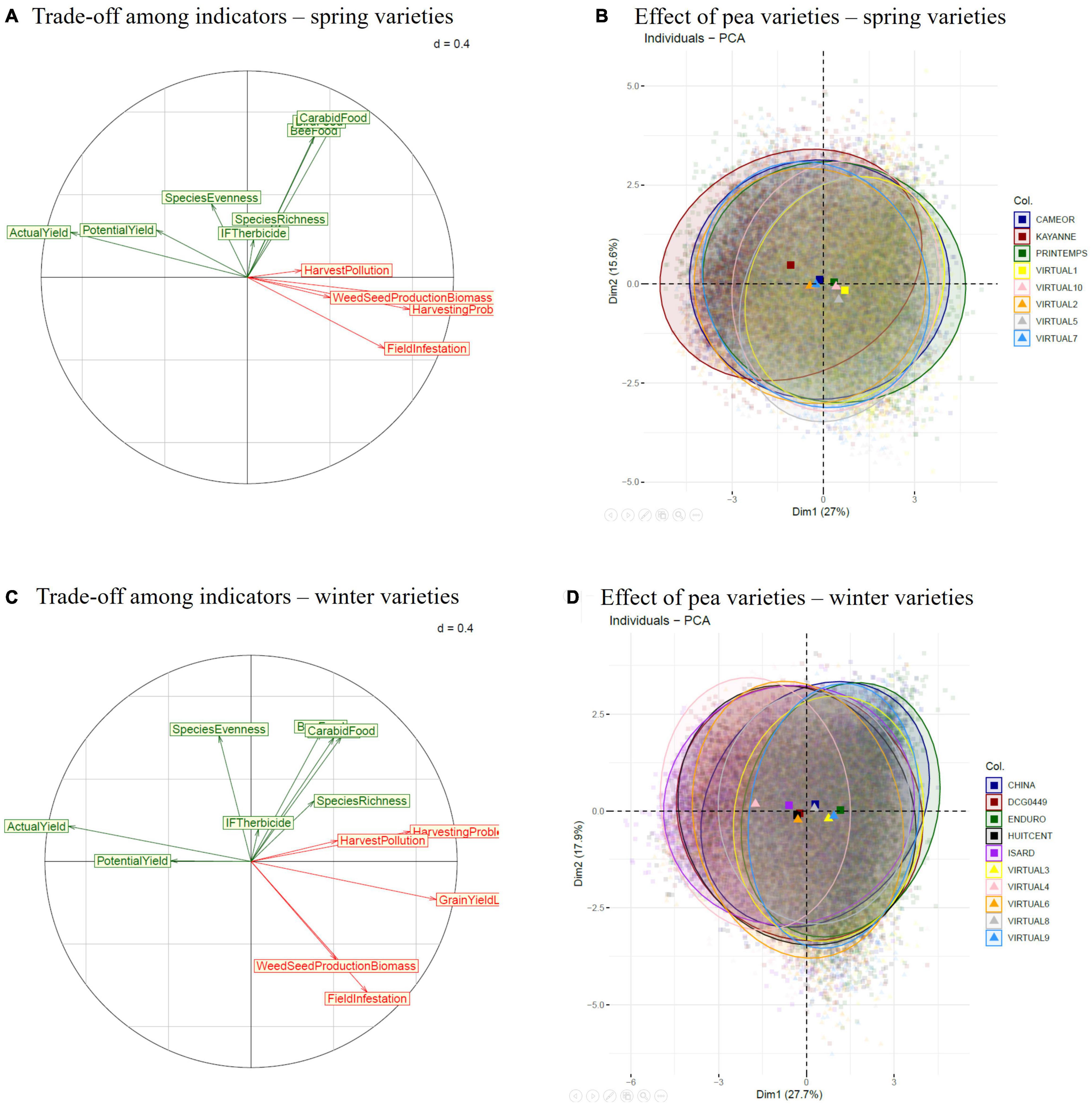
Figure 3. Trade-offs among indicators of pea yield and weed (dis)service identified with Principal Component Analyses (PCA) for spring (A,B) and winter pea varieties (C,D) on the nine simulated situations, using annual simulated data. Pea-yield and biodiversity indicators are shown in green, weed harmfulness for pea production is in red (Colbach, 2020 ).

Pea Varieties Differ in Terms of Yield and Weed (Dis)services

The ellipses corresponding to the different pea varieties were very large, indicating that their performance in terms of pea yield and weed (dis)services varied greatly with the situation, cropping system, year, weather repetition (Figures 3B,D). These ellipses mostly overlapped, indicating that simulation factors other than pea variety explained most of the variability. Despite this, a few tendencies could be observed. In spring pea, varieties were roughly ranked along a line ranging from yield to field infestation (Figure 3B). The best-performing variety was an actual one, i.e., Kayanne, the worst-performing varieties were all virtual ones. Winter pea varieties were ranked roughly along a line from weed-infested yield to yield loss due to weeds, with larger differences among varieties than for spring pea (Figures 3D vs. B). Actual varieties were all outperformed by a virtual one (Virtual 4), and the worst variety was an actual one (Enduro).

The trade-off between pea yield in the absence of weeds (i.e., potential yield) and pea resilience toward weeds (i.e., yield loss due to weeds) as well as crop impact on weeds (i.e., field infestation) was obvious on actual varieties (Table 1B). The variety with the highest potential yield (Isard) was intermediate in terms of yield loss and field infestation. Conversely, the variety with the highest field infestation (Cameor) was intermediate in terms of potential yield and yield loss. The two spring varieties (Cameor and Kayanne) presented the lowest weed-related yield loss and almost the best yield potential. Otherwise, there was no obvious link between average variety-performance indicators and major variety characteristics, i.e., leaf morphology (Cameor, China and DCG0449 did not differ from the rest), seed mass or maximum plant height (no correlation between these two traits and any of the three indicators of Table 1B).

There was also a trade-off between the average performance of actual varieties and their stability across situations, years, and weather repetitions (sd in Table 1B). For instance, the variety with the lowest average potential yield (China) had the second-highest yield stability; the variety with the most stable yield loss (Enduro) was also the one with the highest yield loss. Conversely, the variety with the highest field infestation (Cameor) also presented the most variable one. Generally, spring varieties (Cameor and Kayanne) presented the highest variability, regardless of the analyzed indicator.

Which Simulation Factors Drive Potential Yield and Weed (Dis)services?

The more detailed analysis of the pea-variety impact with the help of the classification and regression trees (CART) showed that this impact greatly varied with the analyzed indicator and scale (Table 3). The more a weed (dis)service indicator was related to crop growth and production, the larger the effect of pea parameters was (larger partial R² in Table 3) and the lower the effects of management techniques and situation were (lower partial R² in Table 3). Potential yield (i.e., from the weed-free simulations) mostly depended on pea parameters (higher partial R² than for other simulation factors in Tables 3A,C). The response of pea to weeds also depended on pea parameters as shown by weed-infested yield and weed-caused yield loss but the latter depended much more on crop management. The effect of pea parameters was even smaller when looking at indicators translating weed response to pea and management, whether quantitative (i.e., field infestation which is based on weed biomass) or qualitative (bee food offer and species richness which are based on weed traits and/or species).

The CART analyses of Table 3 confirmed some tendencies already identified with the Principal Component Analysis of Figure 3. For potential pea yield, pea parameters were more important in spring pea (Table 3A) than in winter pea (Table 3C) and vice-versa for pea techniques; for yield loss, the opposite was true, i.e., pea parameters were most important in winter pea and pea techniques most important in spring pea. Explained variability was smaller for weed-impact indicators than for potential yield, pointing to stronger interactions among simulation factors and to a larger impact of effects that were not included in the analysis, i.e., weather and stochastic effects (e.g., weed plant location). Generally, the effect of both pea parameters and pea management techniques was more visible during the years with pea (Tables 3A,C) than at the rotation scale (Tables 3B,D) where these effects were overshadowed by other-crop techniques. This was particularly true for rotation-scale yields (potential and weed-infested) as these indicators included yield data from crops other than pea. Though the management of crops other than pea was the most influential when analyzing weed (dis)services at the rotation scale, other-crop techniques also influenced both pea yield and, particularly, weed impacts in pea crops at the annual scale (Tables 3A,C).

The effect of simulation factors on the indicators of the composite performance profiles (“Integrated” and “Agroecology”) varied with varieties and scales. But generally, pea parameters were the most important for winter varieties, and pea techniques for spring varieties; the opposite was true for other-crop management. The situation had no effect at the rotation scale, and variability was least well explained for the “Agroecology” profile.

Which Pea Parameters and Techniques Drive Potential Yield and Yield Loss?

Table 4 lists the main pea parameters (Table 4A) and techniques (Table 4B) driving potential yield and weed-caused yield loss in pea as well as the explanations for these effects, based on the functioning of the FLORSYS model. The results on the other-crop techniques, the other weed-impact indicators, and from the rotation scale are in section E of the Supplementary Material. In short, any parameter value which delays and/or reduces crop emergence (e.g., large darknessReduction or gamma values) decreased potential yield and, particularly, yield-loss control. Conversely, any parameter value which increases crop canopy volume (e.g., large LBRlate or mu_HMmid values) and crop growth duration (e.g., large PeaFloweringTT values) had the opposite effect (Table 4A). Shading response (mu parameters) was crucial: the more pea plants increase plant height (large mu_HMmid values) and leaf biomass (large mu_LBRlate) when shaded, the better. However, key parameters completely differed between pea-variety types and indicators: for instance, parameters driving germination and pre-emergent growth were crucial for yield-loss control in winter pea but not in spring pea or for potential yield. Field infestation was little affected (details in section E).

Interestingly, almost all parameters either always increased (probability values in Table 4A = 1) or always decreased indicator values (probability = 0), indicating a stable effect regardless of other parameters and management techniques. Three of the key parameters (darknessReduction, gamma, rb) did not vary among actual varieties as variety-specific information was unavailable when parameterizing pea in FLORSYS. All three concern pre-emergent processes. All other parameters vary as much for virtual as for actual varieties. Generally, the range of variation of the key pea parameters was smaller than the range for other crops and included in this latter range. The only exceptions concern plant morphology: when shaded, pea plants mostly reduced their leaf biomass ratio (mu_LBR < 0) whereas most other crops increase theirs (mu_LBR > 0).

In terms of pea management, the technique driving crop growth duration, i.e., sowing date, was the most influential factor, but its effect depended on the pea variety type and other interactions (Table 4B). Delayed spring-pea sowing deteriorated the control of yield loss and field infestation whereas the effect varied for delayed winter-pea sowing. Field-infestation control systematically decreased but yield potential and yield-loss control usually improved (because of, e.g., less frost damage). All the other key techniques presented a stable effect, irrespective of pea varieties, though the effect could vary (i.e., the probability was not 0 or 1) depending on other conditions (e.g., other management techniques). Potential pea yield mostly depended on a dense (high sowing density) and uniform crop canopy (row sowing, small interrow width) whereas the control of yield loss and field infestation mostly depended on tillage aiming to reduce the weed seed bank, with depth and timing being crucial for success. Herbicides were the most important for field infestation, mechanical weeding for yield loss.

Optimize Pea Varieties and Management

With the help of the classification and regression trees, optimal combinations of pea parameters and crop management techniques were identified, depending on the performance goal, the situation, the pea variety type, and the decision scale (see examples in Figure 2 and Table 5, with the complete set of branches in section F of the Supplementary Material). The examples presented here focused on pea yield, and were chosen to illustrate the impact of weeds, pea variety type, weed-control strategy, and analysis scale.

Maximize Potential Yield in Spring Pea in Herbicide-Based Systems

To optimize potential yield in spring pea in herbicide-based cropping systems, the choice of pea parameters was crucial (Table 5A). A set of common 29 rules described the pea varieties of the three best tree branches, corresponding to respectively the 6, 5, and 5% situations with the highest potential yield among the 35 branches of the tree. For these best configurations, plants photosynthesized well at low temperatures (low tPhoto2). When unshaded, their width increased with increasing biomass after emergence and during reproduction (high b_WMearly and b_WMlate, low WMearly) but it was homogeneous during the vegetative stage (low b_WMmid). Plants were stemmy before reproduction (low LBRearly and LBRmid) but kept investing a large proportion of biomass in leaves during reproduction (high LBRlate) though the leaves were small and thick (low SLAlate). Leaf distribution along plant height was uniform (RLHearly and RLHmid close to 0.5, low b_RLHearly and b_RLHlate), and plants were tall per unit biomass at all stages (large HMearly, HMmid, and HMlate). Shaded plants compensated by investing more biomass into leaves (large mu_LBRlate), with larger thinner leaves (large mu_SLAearly) and became even taller per unit biomass (large mu_HMmid). Growth duration needed to exceed a minimum threshold (PeaFloweringTT), germination was early (low g0, g50) and fast (large gb), leading to well-established seedling (large LA0) (Table 5A). These advantages came at a cost, being linked to less favorable features, such as a reduced root system (low rateCyl), which was moreover sensitive to soil compaction (low soilPen).

Many of these rules were respected by all the actual pea varieties tested here, e.g., a low leaf biomass ratio after emergence (LBRearly < 0.821 g/g) or a minimum time from emergence to flowering (PeaFlwoeringTT ≥ 295°Cdays). The most discriminating rules were the seven that drove the first split in the tree (i.e., order = 1 in the tree). They concern diverse traits such as the ability to photosynthesize at low temperatures (low tPhoto2), to keep a high biomass ratio during reproduction (large LBRlate), or to compensate shading by increasing plant height (large mu_HMmid). In the end, only three varieties verified all 29 rules, i.e., Kayanne, Virtual2, and Virtual 7.

The best two branches consisted of further, opposing 21 rules. Two virtual varieties corresponded to the best branch B1 (Virtual2 and Virtual7). The three branches moreover differed in terms of pea management, with B1 and B2 requiring a narrower interrow than B3. All three branches needed a high sowing density and an early sowing date. Rotation and the management of crops other than pea presented negligible effects.

What Changes in the Presence of Weeds?

When looking at weed-infested yield (Table 5B), the main rules for spring-pea varieties in herbicide-based systems remained the same for the three best branches corresponding to the 2.1% best performances, except that the pea growth period needed to be limited (low PeaFloweringTT). The latter rule cuts off part of weed-seed reproduction and infestation of future crops. In the best two branches, the emphasis was more on high leaf area than for potential yield, to the detriment of root-system expansion. The latter was closer to the soil surface, reducing available water for weed seed germination and emergence. Another difference was a slower crop emergence, which increased the efficiency of pre- and post-sowing herbicides as early emerging weeds would be more exposed to herbicide droplets. The varieties corresponding to the three branches comprised the same three varieties as for potential pea yield, with the additional Cameor variety.

Compared to the weed-free branches, the optimal weed-infested branches considerably differed in terms of rotation and crop management. In pea, tillage and herbicides became more important than sowing patterns. The best branch was characterized by a high crop diversity. Herbicide options were important but not in all crops: if stringent rules were applied in pea (branch B1), none were needed in other crops, and vice versa (B2 and B3).

Are Optimal Parameter Values the Same for Spring vs. Winter Varieties?

The rules for winter pea in herbicide-based systems were completely different (Table 5C) from the spring-pea rules. Winter-pea rules concerned either a fast root-system extension (large rateWidth and rateDepth) and a strong shading response in terms of leaf-biomass increase (large mu_LBRmid) (branches B1 and B2) or a slow root-system extension (low rateWidth and rateDepth), leaving more above-ground biomass for light interception (B3). The latter variety-type though only worked if the weed flora consisted of the six harmful dicots that promote the bee-food offer. The first branches corresponded to two actual varieties (886-1 and DCG0449) and the last one to one actual variety (Isard). Crop-management rules focused on tillage and mechanical weeding, and the discrimination between branches B1 and B2 was based on the delay between the last tillage operation and pea sowing.

What Changes in Herbicide-Free Pea Crops?

The weed-infested yield was higher for unsprayed than for sprayed spring pea, ranging from 0.51 to 0.63 (with 1 = the best weed-infested yield observed for pea in all simulations) for the 6.8% best-unsprayed spring-pea crops (Table 5D) compared to 0.53–0.55 for the 2.1% best-sprayed ones (Table 5B). Two main strategies were identified for unsprayed spring pea (Table 5D). Branch B1 and B2 had few pea-variety rules which were the same as the main rules in sprayed pea. To be successful, these few rules had to be combined with a great many constraints for crop management, mainly in the three most frequent crops (pea, wheat, oilseed rape). Conversely, branch B3 mainly focused on mechanical weeding but compensated with additional pea-variety rules, ensuring early crop establishment (in contrast to sprayed systems where this reduced herbicide efficiency), a better light interception by the crop, and more shading of weeds.

What Changes in Untilled Pea Crops?

In untilled spring pea, only the main usual 7–8 variety rules were useful (Table 5E). This resulted in a lower weed-infested yield (0.46–0.54 for the 3.4% best-untilled systems) than in either sprayed (Table 5B) or unsprayed pea (Table 5E). The best branch B1 was based on high-density pea and needed few other management rules, except on wheat varieties and herbicides at the rotation scale. But, the other two branches, with their lower pea densities, needed many other management rules, either at the rotation scale or specifically for the two most frequent crops, wheat, and oilseed rape. In all three branches, herbicide rules were crucial.

Do Rotation-Scale Analyses Lead to the Same Conclusions?

If the performance was analyzed at the rotation scale, the pea-parameter rules did not change, here is the example of continuously untilled cropping systems (Table 5F) compared to untilled pea and analysis focusing on pea yield only. The main difference concerned herbicides: these became even more crucial at the scale of the no-till system and/or in the two most frequent crops than when analyzing untilled pea.

To Which Extent Ideal Varieties Can Help to Reach Multi-Performance?

When more goals were included in the approach, e.g., reduced herbicide use and improved bee-food offer in addition to yield-loss control, the focus shifted from pea parameters to crop management throughout the rotation (particularly herbicide options, details in section F of the Supplementary Material). Because of the trade-off between biodiversity promotion and harmfulness control, no optimal branches reconciling all these goals could be identified. The best options improved yield (normed yield = 0.38–0.53) and reduced herbicide use (normed = 0.78–1, note that 1 corresponds to zero use) but bee food offer remained stubbornly low (normed = 0.07–0.15). Even the branch with the best bee food, this offer remained low (0.22) and came with a high price in terms of pea yield (0.1).

Conclusion

In conclusion, the main pea-parameter rules were the same for all performance goals, management strategies, and analyses scales, stressing the importance of early field occupation and shade response aiming to increase plant height and leaf area. However, further different rules were useful for individual goals, strategies, and scales. Some variety features only fitted to particular systems (e.g., delayed pea emergence is only advantageous in case of spraying and disastrous in unsprayed systems). Fewer parameter rules usually had to be compensated by more management rules. Similarly, if one of the two main weed-control levers, herbicide or tillage, was eliminated, further pea-parameter and/or management rules were needed.

Discussion

What Is New?

In the present paper, we combined detailed experimental measurements characterizing varieties with a simulation study to test actual and virtual varieties in virtual field networks in the example of pea, in order to identify ideotypes of varieties and cropping systems for agroecological weed management. This approach was inspired by our previous paper (Colbach et al., 2019) focusing on inter-species instead of intra-species differences, where we already discussed the novelty of this approach as well as its advantages and limits, in terms of variability of investigated situations, use of parameters reflecting intrinsic plant properties that vary little with the environment, and lower risk of confusion effects.

Here, we went several steps further to (1) include all species parameters instead of focusing on plant morphology and shading response, (2) shift from the species to the variety scale, and to (3) identify relevant crop parameters and, particularly, parameter combinations not only for a given production goal but also for contrasting cropping-system types. The present study differed in another key point: it not only aimed to determine ideotypes of varieties but also (4) ideotypes of crop management plans and cropping systems. Working at the cropping-system scale is particularly novel. Though ecophysiologists design ideotypes for different agronomic and pedoclimatic conditions and they even use sowing strategies (e.g., density, interrow width) to achieve ideal plant morphology via morphological plasticity, they usually disregard multiannual effects (Martre et al., 2015).

In terms of methodology, we shifted from real-life cropping systems and crops in our previous paper (Colbach et al., 2019) to virtual (randomized) systems and varieties in the present study, to explore a larger range of parameters/techniques and their combinations. The Latin Hypercube Sampling (LHS) plan for the simulation plan was particularly appropriate for this objective, as it was shown here to both decorrelate management variables (thus reducing the risk of confusing effects) and respect biological correlations among variety characteristics (thus avoiding biological nonsense).

The conclusion of our previous study comparing different species was very similar (Colbach et al., 2019). In addition to “generalist winners” (resulting from the main 7–8 rules identified in all spring-pea cases of Table 5), the present study also searched for ideotypes fine-tuned to individual situations (e.g., with or without herbicides) and variety types (spring vs. winter). Though the main parameter rules remained the same, the “specialized winners” greatly varied, in terms of relevant parameters and parameter combinations, parameter thresholds, and impacts on crop yield and weed (dis)services. Notably, combinations of minor parameters could be more efficient than a single optimum dominant one, particularly if combined with adapted crop management. This makes work more difficult, both for crop breeders (who need to produce contrasting varieties) and farmers (who need to identify the best variety for their production context).

Are the Results Consistent With Previous Studies?

Our results are conditional on the prediction quality of FLORSYS which was shown to be adequate in a previous study (section “Domain of Validity”). In our previous simulation study, we further checked the consistency of simulated yield loss regarding weed and crop species and parameters, concluding that the species rankings and features identified as relevant were consistent with the literature (Colbach et al., 2019). Here, we specifically searched the literature for pea studies (Table 6). Generally, both our experimental and simulation results agree with the few literature reports on pea.

TABLE 6

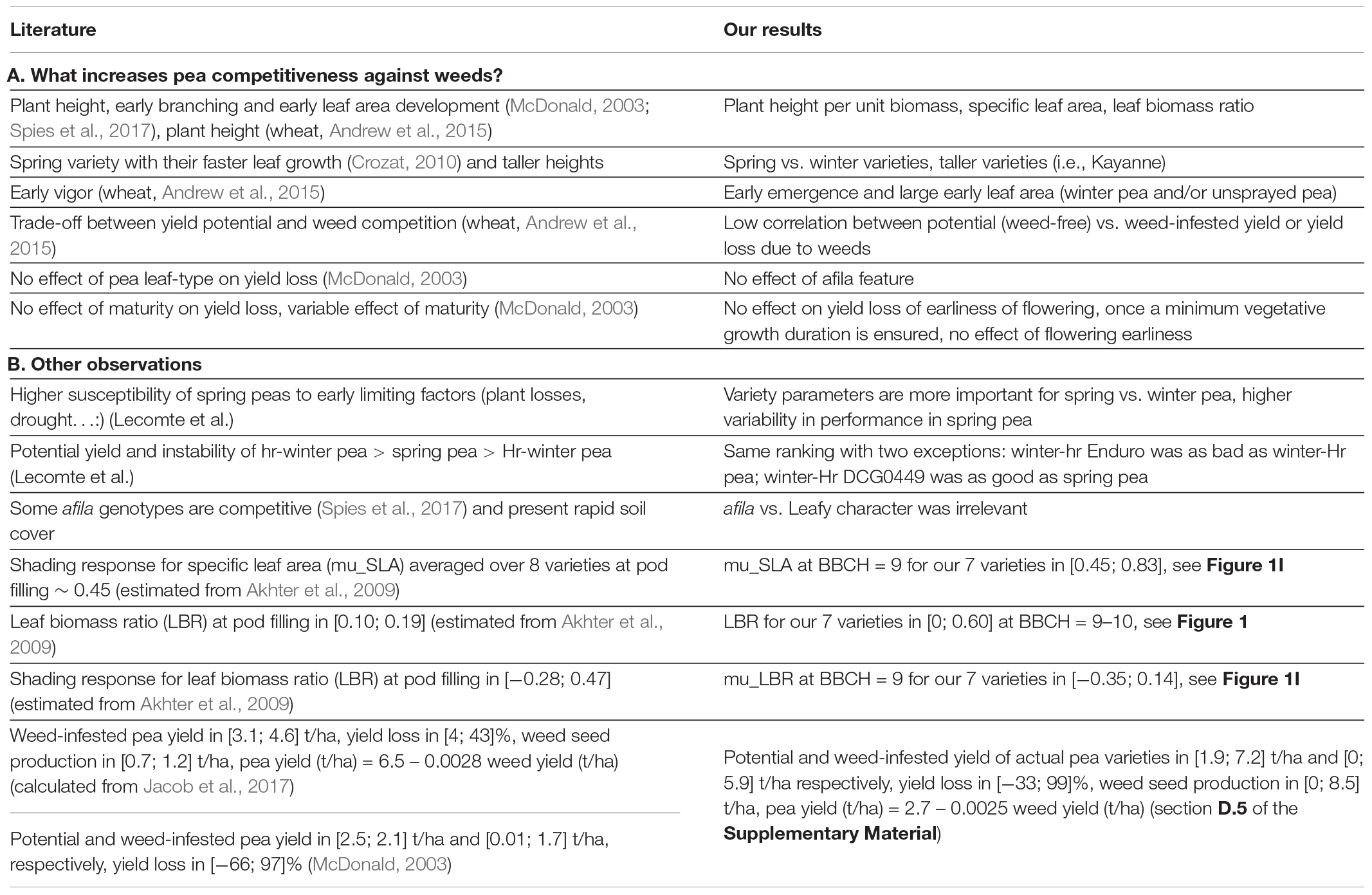
Table 6. Consistency of present results compared to literature reports.

There were some discrepancies. For instance, the DCG0449 had a potential yield as high as the best spring pea variety in our study whereas field observations report that winter-Hr varieties such as DCG0449 present the lowest yield potential among all pea variety types because of their late maturity which exposes them to end-of-cycle stresses and by a higher susceptibility to diseases and lodging (Lecomte et al., in prep). Conversely, Enduro performed badly here in contrast to field studies which report yield similar to that of the other winter-hr variety, Isard. Our study showed that the genotypes were highly contrasted between and within pea types, and that seasonality (winter vs. spring and Hr vs. hr), leaf morphology (leafy vs. afila), and usage (protein vs. forage) are insufficient to characterize them.

As in field studies, the present simulation study demonstrated the effect of pea parameters on yield and competitiveness against weeds. However, it is difficult to compare these field reports to our pea parameters which were chosen to be independent of location (e.g., plant height per unit biomass in unstressed conditions) whereas most field-measured variables (e.g., plant height) are also the result of environmental conditions. Some mental arithmetic is needed to conclude how far our results are consistent with field reports (Table 6). Some appear contradictory at first glance, such as the higher yields and lower yield losses reported by Jacob et al. (2017). However, their weed infestation was much lower than ours, demonstrated by their lower weed seed production. Despite these differences, the slope linking pea yield and weed seed production was very similar in their experiments and our simulations. Moreover, other field observations reported lower pea yields, and yield loss ranges similar to ours (McDonald, 2003).

Implications for Farmers and Crop Breeders

The identification of the parameters relevant for yield and weed control is a major stepping-stone toward decision support for farmers. The take-home message for pea varieties in the present study was the importance of early field occupation and shade response, though the exact features (nature and values of relevant parameters) depend on the targeted weed impacts. The next step will screen the existing pea varieties and identify those similar to the ideotypes. However, many of the parameters used here are not routinely measured during breeding (Zhao et al., 2006) and are estimated in controlled conditions (e.g., Gardarin et al., 2010) or on individual plants in garden plots as in section “Parameterizing Contrasting Pea Varieties.” This would mean retesting all varieties with the help of, e.g., high-throughput phenotyping platforms (Jeudy et al., 2016; Brichet et al., 2017).

The actual pea varieties tested here were not very good at controlling weeds. As at the species scale (Colbach et al., 2019), we found again that varieties or parameters that increase potential yield are not necessarily those that minimize weed-caused yield loss. This is often explained by a trade-off between community performance and competitiveness (Denison et al., 2003). But, even though this is a frequently reported antagonism (Sardana et al., 2017), it is not inevitable as shown by recent varietal improvement in rice (Mahajan et al., 2014, 2015). The low weed-control ability of the current pea varieties probably reflects past breeding history where the focus was on potential yield or disease resistance rather than competitiveness against weeds (Tayeh et al., 2015). The present results (particularly the pea-parameter rankings in section E of the Supplementary Material) are a starting point to guide crop breeders toward more competitive pea varieties.

Some features identified here are not consistent with current breeding trends. For instance, a longer crop growth duration tended to improve pea performance here whereas breeding programs currently aim to shorten the pea crop cycle in order to escape to limiting factors of the end of the crop cycle (high temperatures, water deficit), especially for spring and Hr-winter peas, whose cycle is positioned later than hr-winter peas. This points to one of the limits of the present study, which considered water to be non-limiting after plant emergence. Conversely, the present results do not question the current preference for afila varieties, which perform better with respect to diseases and lodging, as this parameter was not relevant here for weed regulation.

From Theory to Practice: What Remains to Be Done?

The pea-parameter rankings of section E of the Supplementary Material and the optimal parameter-value × technique combinations of section F of the Supplementary Material are a first essential step for decision support to both crop breeders and farmers, proposing varieties for agroecological weed management depending on the cropping-system type and performance goal. Or, vice-versa, rules for adapting crop management to a given variety that was chosen, for instance, for protein content rather than for weed control. For practical use, the parameter rankings and decision trees must be transformed into an actual decision support system, which must be specified with future users, notably concerning the way these results should be visually represented in a graphical user interface.

“Packaging” is not the only issue. As mentioned in section “Implications for Farmers and Crop Breeders,” neither the here-tested virtual varieties nor the identified optimal parameter-value × technique combinations scored highly when attempting to achieve both high potential yield and high yield loss control (and even worse when adding other goals). Possibly, we simply missed the “winning” varieties as we only assessed seven actual and 10 virtual ones. To specifically search for these winners, if they exist, or to build a set of trade-off solutions that would be used by stakeholders to choose a compromise according to their constraints, optimization algorithms could be used (Press et al., 2007; Venter, 2010).

Another limitation of the applicability of the present results is that many of our parameters are difficult to measure (particularly those related to plant morphology and shading response) and are not routinely measured by plant breeders (Zhao et al., 2006). A solution would be to link our parameters (which are usually measured in controlled conditions and/or isolated plants) to routinely measured features and, if necessary, propose additional measurements that are easily carried out on dense canopies in field trials during varietal selection and testing. The same approach was already used at the species scale to estimate many of FLORSYS’ most difficult parameters (e.g., Gardarin et al., 2012; Colbach et al., 2020b) but has not yet been attempted at the within-species scale. Recent advances in artificial intelligence and image analysis will also be helpful, such as the correlation established recently between destructive measurements of above-ground biomass and contactless measurements of leaf area (Gée et al., 2021). New techniques for image segmentation (artificial convolutional neural networks) will also be crucial to discriminate different species (Bateman et al., 2020).

The present study focused on crop-weed competition for the light which is generally the main resource for which crops and weeds compete in conventional cropping systems (Wilson and Tilman, 1993; Perry et al., 2003). But with the current limitation of nitrogen fertilizer for environmental reasons (Swarbreck et al., 2019), crop-weed competition for nitrogen will become more prevalent. Moreover, as a nitrogen-fixating legume crop, pea will have a major advantage over weeds, at least in temperate cropping systems where there are no Fabaceae weeds. Such a study will soon be possible with the recent introduction of crop-weed competition for nitrogen into FLORSYS (Moreau et al., 2021).

Finally, the present simulation study was run in a single region, albeit with different weather series and weed floras. As variety performance has been shown to vary among regions and years (McDonald, 2003; Jacob et al., 2017), our study must now be repeated in other pedoclimates to adapt the selection and farming guidelines. These will probably vary, as they do here among cropping systems.

Conclusion

The present sensitivity analysis of pea production and biological weed regulation to pea variety and crop management identified the key parameters that drive potential yield and competitivity against weeds in pea, depending on variety type and cropping system. These are pointers for selecting pea varieties in agroecological cropping systems aiming to regulate weeds by biological interactions. We also produced rules to guide farmers (1) to choose the best pea variety, depending on the production goal and the cropping system, and (2) to adapt crop management to a given pea variety and production goal. The present methodology can be applied to identify ideotypes for weed management in other crops or even crop mixtures. Further research is needed to resolve the trade-off between pea parameters that promote potential yield and those driving weed suppression and to link model parameters to variables routinely measured during crop breeding.

Data Availability Statement

The raw data supporting the conclusions of this article will be made available by the authors, without undue reservation.

Author Contributions

NC and DM designed and led the research. EF, LL, and FS carried out the experiments and measurements. AK and CL provided expert advice. CG performed the image analysis. NC and JV ran the simulations and analyzed the data. TM provided expert advice. NC and DM wrote the draft manuscript with the help of CL. All authors contributed to the article and approved the submitted version.

Funding

This project was supported by INRAE, the French National Research Agency (ANR) Project Investissements d’Avenir PeaMUST (Adaptation Multistress des Protéagineux) under the grant number ANR-11-BTBR-0002, the European Union’s Horizon 2020 research and innovation program under grant agreement N 727217 (ReMIX project), and the Casdar RAID project funded by the French Ministry in charge of Agriculture and Food (Ministère de l’Agriculture et de l’Alimentation, avec la contribution financière du compte d’affectation spéciale ‘Développement agricole et rural’).

Conflict of Interest

The authors declare that the research was conducted in the absence of any commercial or financial relationships that could be construed as a potential conflict of interest.

Publisher’s Note

All claims expressed in this article are solely those of the authors and do not necessarily represent those of their affiliated organizations, or those of the publisher, the editors and the reviewers. Any product that may be evaluated in this article, or claim that may be made by its manufacturer, is not guaranteed or endorsed by the publisher.

Supplementary Material

The Supplementary Material for this article can be found online at: https://www.frontiersin.org/articles/10.3389/fpls.2022.809056/full#supplementary-material

Footnotes

1. ^ https://agreste.agriculture.gouv.fr/

References

Akhter, N., Rahman, M., Hasanuzzaman, M., and Nahar, K. (2009). Physiological response of garden pea (Pisum sativum L.) grown under different light environment. Bot. Res. Int. 2, 304–309.

Google Scholar

Andrew, I. K. S., Storkey, J., and Sparkes, D. L. (2015). A review of the potential for competitive cereal cultivars as a tool in integrated weed management. Weed Res. 55, 239–248. doi: 10.1111/wre.12137

PubMed Abstract | CrossRef Full Text | Google Scholar

Bastiaans, L., Kropff, M. J., Kempuchetty, N., Rajan, A., and Migo, T. R. (1997). Can simulation models help design rice cultivars that are more competitive against weeds? Field Crops Res. 51, 101–111. doi: 10.1016/S0378-4290(96)01046-5

CrossRef Full Text | Google Scholar

Bateman, C. J., Fourie, J., Hsiao, J., Irie, K., Heslop, A., Hilditch, A., et al. (2020). Assessment of mixed sward using context sensitive convolutional neural networks. Front. Plant Sci. 11:159. doi: 10.3389/fpls.2020.00159

PubMed Abstract | CrossRef Full Text | Google Scholar

Breiman, L., Friedman, J. H., Olshen, R. A., and Stone, C. J. (1984). Classification and Regression Trees. New York, NY: Chapman and Hall.

Google Scholar

Brichet, N., Fournier, C., Turc, O., Strauss, O., Artzet, S., Pradal, C., et al. (2017). A robot-assisted imaging pipeline for tracking the growths of maize ear and silks in a high-throughput phenotyping platform. Plant Methods 13:96. doi: 10.1186/s13007-017-0246-7

PubMed Abstract | CrossRef Full Text | Google Scholar

Brisson, N., Gary, C., Justes, E., Roche, R., Mary, B., Ripoche, D., et al. (2003). An overview of the crop model STICS. Eur. J. Agron. 18, 309–332.

Google Scholar

Brisson, N., Launay, M., Mary, B., and Beaudoin, N. (2009). Conceptual Basis, Formalisations and Parameterization of the STICS Crop Model. Versailles: Éditions Quae.

Google Scholar

Burstin, J., Salloignon, P., Chabert-Martinello, M., Magnin-Robert, J.-B., Siol, M., Jacquin, F., et al. (2015). Genetic diversity and trait genomic prediction in a pea diversity panel. BMC Genomics 16:105. doi: 10.1186/s12864-015-1266-1

PubMed Abstract | CrossRef Full Text | Google Scholar

Castel, T., Lecomte, C., Richard, Y., Lejeune-Hénaut, I., and Larmure, A. (2017). Frost stress evolution and winter pea ideotype in the context of climate warming at a regional scale. OCL 24:D106. doi: 10.1051/ocl/2017002

CrossRef Full Text | Google Scholar

Chauvel, B., Guillemin, J. P., Colbach, N., and Gasquez, J. (2001). Evaluation of cropping systems for management of herbicide-resistant populations of blackgrass (Alopecurus myosuroides Huds.). Crop Protect. 20, 127–137.

Google Scholar

Christensen, S. (1995). Weed suppression ability of spring barley varieties. Weed Res. 35, 241–247. doi: 10.1111/j.1365-3180.1995.tb01786.x

CrossRef Full Text | Google Scholar

Colbach, N., Bertrand, M., Busset, H., Colas, F., Dugué, F., Farcy, P., et al. (2016). Uncertainty analysis and evaluation of a complex, multi-specific weed dynamics model with diverse and incomplete data sets. Environ. Model. Softw. 86, 184–203. doi: 10.1016/j.envsoft.2016.09.020

CrossRef Full Text | Google Scholar

Colbach, N., Busset, H., Roger-Estrade, J., and Caneill, J. (2014a). Predictive modelling of weed seed movement in response to superficial tillage tools. Soil Tillage Res. 138, 1–8. doi: 10.1016/j.still.2013.12.002

CrossRef Full Text | Google Scholar

Colbach, N., Collard, A., Guyot, S. H. M., Mézière, D., and Munier-Jolain, N. M. (2014b). Assessing innovative sowing patterns for integrated weed management with a 3D crop:weed competition model. Eur. J. Agron. 53, 74–89. doi: 10.1016/j.eja.2013.09.019

CrossRef Full Text | Google Scholar

Colbach, N., Petit, S., Chauvel, B., Deytieux, V., Lechenet, M., Munier-Jolain, N., et al. (2020c). The pitfalls of relating weeds, herbicide use, and crop yield: don’t fall into the trap! A critical review. Front. Agron. 2:615470. doi: 10.3389/fagro.2020.615470

CrossRef Full Text | Google Scholar

Colbach, N., Chauvel, B., Messéan, A., Villerd, J., and Bockstaller, C. (2020a). Feeding pollinators from weeds could promote pollen allergy. A simulation study. Ecol. Indic. 117:106635. doi: 10.1016/j.ecolind.2020.106635

CrossRef Full Text | Google Scholar

Colbach, N., Moreau, D., Dugué, F., Gardarin, A., Strbik, F., and Munier-Jolain, N. (2020b). The response of weed and crop species to shading. How to predict their morphology and plasticity from species traits and ecological indexes? Eur. J. Agron. 121:126158. doi: 10.1016/j.eja.2020.126158

CrossRef Full Text | Google Scholar

Colbach, N., Colas, F., Cordeau, S., Maillot, T., Queyrel, W., Villerd, J., et al. (2021). The FLORSYS crop-weed canopy model, a tool to investigate and promote agroecological weed management. Field Crops Res. 261:108006. doi: 10.1016/j.fcr.2020.108006

CrossRef Full Text | Google Scholar

Colbach, N., and Cordeau, S. (2018). Reduced herbicide use does not increase crop yield loss if it is compensated by alternative preventive and curative measures. Eur. J. Agron. 94, 67–78. doi: 10.1016/j.eja.2017.12.008

CrossRef Full Text | Google Scholar

Colbach, N., and Debaeke, P. (1998). Integrating crop management and crop rotation effects into models of weed population dynamics: a review. Weed Sci. 46, 717–728. doi: 10.1017/S0043174500089761

CrossRef Full Text | Google Scholar

Colbach, N., Gardarin, A., and Moreau, D. (2019). The response of weed and crop species to shading: which parameters explain weed impacts on crop production? Field Crops Res. 238, 45–55. doi: 10.1016/j.fcr.2019.04.008

CrossRef Full Text | Google Scholar

Crozat, Y. (2010). “Biotic stresses, weeds,” in Physiologie of the Pea Crop, eds N. G. Munier-Jolain, V. Biarnès, I. Chaillet, J. Lecoeur, and M. H. Jeuffroy (Versailles: Éditions Quae), 197–198.

Google Scholar

Denison, R. F., Kiers, E. T., and West, S. A. (2003). Darwinian agriculture: when can humans find solutions beyond the reach of natural selection? Q. Rev. Biol. 78, 145–168. doi: 10.1086/374951

PubMed Abstract | CrossRef Full Text | Google Scholar

Drews, S., Neuhoff, D., and Köpke, U. (2009). Weed suppression ability of three winter wheat varieties at different row spacing under organic farming conditions. Weed Res. 49, 526–533. doi: 10.1111/j.1365-3180.2009.00720.x

CrossRef Full Text | Google Scholar

Duc, G., Agrama, H., Bao, S., Berger, J., Bourion, V., De Ron, A. M., et al. (2015). Breeding annual grain legumes for sustainable agriculture: new methods to approach complex traits and target new cultivar ideotypes. Crit. Rev. Plant Sci. 34, 381–411. doi: 10.1080/07352689.2014.898469

CrossRef Full Text | Google Scholar

Espósito, M. A., Martin, E. A., Cravero, V. P., and Cointry, E. (2007). Characterization of pea accessions by SRAP’s markers. Sci. Hortic. 113, 329–335. doi: 10.1016/j.scienta.2007.04.006

CrossRef Full Text | Google Scholar

Ford, G. T., and Pleasant, J. M. (1994). Competitive abilities of six corn (Zea mays L.) hybrids with four weed control practices. Weed Technol. 8, 124–128. doi: 10.1017/S0890037X00039312

CrossRef Full Text | Google Scholar

Fried, G., Norton, L. R., and Reboud, X. (2008). Environmental and management factors determining weed species composition and diversity in France. Agric. Ecosyst. Environ. 128, 68–76. doi: 10.1016/j.agee.2008.05.003

CrossRef Full Text | Google Scholar

Gardarin, A., Dürr, C., and Colbach, N. (2010). Effects of seed depth and soil structure on the emergence of weeds with contrasted seed traits. Weed Res. 50, 91–101. doi: 10.1111/j.1365-3180.2009.00757.x

CrossRef Full Text | Google Scholar

Gardarin, A., Dürr, C., and Colbach, N. (2012). Modeling the dynamics and emergence of a multispecies weed seed bank with species traits. Ecol. Model. 240, 123–138. doi: 10.1016/j.ecolmodel.2012.05.004

CrossRef Full Text | Google Scholar

Gée, C., Denimal, E., Merienne, J., and Larmure, A. (2021). Evaluation of weed impact on wheat biomass by combining visible imagery with a plant growth model: towards new non-destructive indicators for weed competition. Precision Agric. 22, 550–568. doi: 10.1007/s11119-020-09776-6

CrossRef Full Text | Google Scholar

Glenn De’ath (2014). Beth Atkinson. R Port of Rpart by Brian Ripley <ripley@stats.ox.ac.uk>. Some Routines from Vegan – Jari Oksanen<jari.oksanen@oulu.fi> Extensions and Adaptations of rpart to mvpart by Glenn De’ath. “mvpart: Multivariate partitioning”, R. R package version 1.6-2 ed.

Google Scholar

Jacob, C. E., Johnson, E. N., Dyck, M. F., and Willenborg, C. J. (2017). Evaluating the competitive ability of semileafless field pea cultivars. Weed Sci. 64, 137–145.

Google Scholar

Jeudy, C., Adrian, M., Baussard, C., Bernard, C., Bernaud, E., Bourion, V., et al. (2016). RhizoTubes as a new tool for high throughput imaging of plant root development and architecture: test, comparison with pot grown plants and validation. Plant Methods 12:18. doi: 10.1186/s13007-016-0131-9

PubMed Abstract | CrossRef Full Text | Google Scholar

Jeuffroy, M.-H., Vocanson, A., Roger-Estrade, J., and Meynard, J.-M. (2012). The use of models at field and farm levels for the ex ante assessment of new pea genotypes. Eur. J. Agron. 42, 68–78. doi: 10.1016/j.eja.2012.04.005

CrossRef Full Text | Google Scholar

Lecomte, C., Giraud, A., and Aubert, V. (2003). Testing a predicting model for frost resistance of winter wheat under natural conditions. Agronomie 23, 51–66. doi: 10.1051/agro:2002068

CrossRef Full Text | Google Scholar

Lecomte, C., Richer, V., Gauffreteau, A., Jeuffroy, M., Klein, A., Bouviala, M., et al. (in prep). Potential yield and specific limiting factors determined for three pea types (Pisum sativum L.) using the DiagVar-Pea method. Agron. Sustain. Dev.

Google Scholar

Lewis, J. (1973). Longevity of crop and weed seeds: survival after 20 years in soil. Weed Res. 13, 179–191. doi: 10.1111/j.1365-3180.1973.tb01262.x

CrossRef Full Text | Google Scholar

Mahajan, G., Ramesha, M. S., and Chauhan, B. S. (2014). Response of rice genotypes to weed competition in dry direct-seeded rice in India. Sci. World J. 2014:8. doi: 10.1155/2014/641589

PubMed Abstract | CrossRef Full Text | Google Scholar

Mahajan, G., Ramesha, M. S., and Chauhan, B. S. (2015). Genotypic differences for water use efficiency and weed competitiveness in dry direct-seeded rice (Oryza sativa L.). Agron. J. 107, 1573–1583. doi: 10.2134/agronj14.0508

CrossRef Full Text | Google Scholar

Martre, P., Quilot-Turion, B., Luquet, D., Memmah, M., Chenu, K., and Debaeke, P. (2015). Model-Assisted Phenotyping and Ideotype Design. London: Academic Press Ltd-Elsevier Science Ltd. doi: 10.1016/B978-0-12-417104-6.00014-5

CrossRef Full Text | Google Scholar

McDonald, G. K. (2003). Competitiveness against grass weeds in field pea genotypes. Weed Res. 43, 48–58. doi: 10.1046/j.1365-3180.2003.00316.x

CrossRef Full Text | Google Scholar

Memmah, M. M., Quilot-Turion, B., and Rolland, A. (2014). Multicriteria sorting methods to select virtual peach ideotypes. Int. J. Multicriteria Dec. Mak. 4, 348–366. doi: 10.1504/IJMCDM.2014.066874

PubMed Abstract | CrossRef Full Text | Google Scholar

Mennan, H., and Zandstra, B. H. (2005). Effect of wheat (Triticum aestivum) cultivars and seeding rate on yield loss from Galium aparine (cleavers). Crop Protect. 24, 1061–1067. doi: 10.1016/j.cropro.2005.02.012

CrossRef Full Text | Google Scholar

Mézière, D., Petit, S., Granger, S., Biju-Duval, L., and Colbach, N. (2015). Developing a set of simulation-based indicators to assess harmfulness and contribution to biodiversity of weed communities in cropping systems. Ecol. Indic. 48, 157–170. doi: 10.1016/j.ecolind.2014.07.028

CrossRef Full Text | Google Scholar

Moreau, D., Pointurier, O., Perthame, L., Beaudoin, N., Villerd, J., and Colbach, N. (2021). Integrating plant-plant competition for nitrogen into a 3D individual-based model simulating the effects of cropping systems on weed dynamics. Field Crops Res. 268:108166. doi: 10.1016/j.fcr.2021.108166

CrossRef Full Text | Google Scholar

Munier-Jolain, N. M., Collard, A., Busset, H., Guyot, S. H. M., and Colbach, N. (2014). Investigating and modelling the morphological plasticity of weeds in multi-specific canopies. Field Crops Res. 155, 90–98. doi: 10.1016/j.fcr.2013.09.018

CrossRef Full Text | Google Scholar

Munier-Jolain, N. M., Guyot, S. H. M., and Colbach, N. (2013). A 3D model for light interception in heterogeneous crop:weed canopies. Model structure and evaluation. Ecol. Model. 250, 101–110. doi: 10.1016/j.ecolmodel.2012.10.023

CrossRef Full Text | Google Scholar

Nemecek, T., von Richthofen, J.-S., Dubois, G. T., Casta, P., Charles, R. L., and Pahl, H. (2008). Environmental impacts of introducing grain legumes into European crop rotations. Eur. J. Agron. 28, 380–393. doi: 10.1016/j.eja.2007.11.004

CrossRef Full Text | Google Scholar

Otsu, N. (1979). Threshold selection method from gray-level histograms. IEEE Trans. Syst. Man Cybern. 9, 62–66. doi: 10.1109/TSMC.1979.4310076

CrossRef Full Text | Google Scholar

Perry, L. G., Neuhauser, C., and Galatowitsch, S. M. (2003). Founder control and coexistence in a simple model of asymmetric competition for light. J. Theor. Biol. 222, 425–436. doi: 10.1016/S0022-5193(03)00055-9

CrossRef Full Text | Google Scholar

Pointurier, O., Moreau, D., Pagès, L., Caneill, J., and Colbach, N. (2021). Individual-based 3D modelling of root systems in heterogeneous plant canopies at the multiannual scale. Case study with a weed dynamics model. Ecol. Model. 440:109376. doi: 10.1016/j.ecolmodel.2020.109376

CrossRef Full Text | Google Scholar

Press, W. H., Teukolsky, S. A., Vetterling, W. T., and Flannery, B. P. (2007). Numerical Recipes: The Art of Scientific Computing, 3rd Edn. New York, NY: Cambridge University Press.

Google Scholar

R Core Team (2016). R: A Language and Environment for Statistical Computing. Vienna: R Foundation for Statistical Computing.

Google Scholar

R Core Team (2021). R: A Language and Environment for Statistical Computing. Vienna: R Foundation for Statistical Computing.

Google Scholar

Ratnadass, A., Fernandes, P., Avelino, J., and Habib, R. (2012). Plant species diversity for sustainable management of crop pests and diseases in agroecosystems: a review. Agron. Sustain. Dev. 32, 273–303. doi: 10.1007/s13593-011-0022-4

CrossRef Full Text | Google Scholar

Raveneau, M. P., Coste, F., Moreau-Valancogne, P., Lejeune-Hénaut, I., and Dürr, C. (2011). Pea and bean germination and seedling responses to temperature and water potential. Seed Sci. Res. 21, 205–213. doi: 10.1017/S0960258511000067

CrossRef Full Text | Google Scholar

Renton, M. (2013). Shifting focus from the population to the individual as a way forward in understanding, predicting and managing the complexities of evolution of resistance to pesticides. Pest Manag. Sci. 69, 171–175. doi: 10.1002/ps.3341

PubMed Abstract | CrossRef Full Text | Google Scholar

Saltelli, A., Chan, K., and Scott, E. M. (2000). Sensitivity Analysis. Chichester: John Wiley & Sons.

Google Scholar

Sardana, V., Mahajan, G., Jabran, K., and Chauhan, B. S. (2017). Role of competition in managing weeds: an introduction to the special issue. Crop Protect. 95, 1–7. doi: 10.1016/j.cropro.2016.09.011

CrossRef Full Text | Google Scholar

Siol, M., Jacquin, F., Chabert-Martinello, M., Smýkal, P., Le Paslier, M.-C., Aubert, G., et al. (2017). Patterns of genetic structure and linkage disequilibrium in a large collection of pea germplasm. G3 Genes| Genomes| Genetics 7:2461. doi: 10.1534/g3.117.043471

PubMed Abstract | CrossRef Full Text | Google Scholar

Smýkal, P., Aubert, G., Burstin, J., Coyne, C. J., Ellis, N. T. H., Flavell, A. J., et al. (2012). Pea (Pisum sativum L.) in the genomic era. Agronomy 2, 74–115. doi: 10.3390/agronomy2020074

CrossRef Full Text | Google Scholar

Spies, J. M., Warkentin, T. D., and Shirtliffe, S. J. (2017). Variation in field pea (Pisum sativum) cultivars for basal branching and weed competition. Weed Sci. 59, 218–223. doi: 10.1614/WS-D-10-00079.1

CrossRef Full Text | Google Scholar

Swarbreck, S. M., Wang, M., Wang, Y., Kindred, D., Sylvester-Bradley, R., Shi, W., et al. (2019). A roadmap for lowering crop nitrogen requirement. Trends Plant Sci. 24, 892–904. doi: 10.1016/j.tplants.2019.06.006

PubMed Abstract | CrossRef Full Text | Google Scholar

Tao, F., Rötter, R. P., Palosuo, T., Díaz-Ambron, C. G. H., Mínguez, M. I., Semenov, M. A., et al. (2017). Designing future barley ideotypes using a crop model ensemble. Eur. J. Agron. 82, 144–162. doi: 10.1016/j.eja.2016.10.012

CrossRef Full Text | Google Scholar

Tayeh, N., Aubert, G., Pilet-Nayel, M.-L., Lejeune-Hénaut, I., Warkentin, T. D., and Burstin, J. (2015). Genomic tools in pea breeding programs: status and perspectives. Front. Plant Sci. 6:1037. doi: 10.3389/fpls.2015.01037

PubMed Abstract | CrossRef Full Text | Google Scholar

Varela Nicola, F. (2017). Découverte De L’agriculture Française, Détermination de la Température de Base de Plusieurs Variétés De Pois et Participation à des Expérimentations en Serre et au Champ de l’UMR Agroécologie. Dijon: AgroSup ARFAGRI.

Google Scholar

Venter, G. (2010). “Review of optimization techniques,” in Encyclopedia of Aerospace Engineering, eds R. Blockley and W. Shyy (Chichester: John Wiley & Sons Ltd).

Google Scholar

Vocanson, A., and Jeuffroy, M.-H. (2008). Agronomic performance of different pea cultivars under various sowing periods and contrasting soil structures. Agron. J. 100, 748–759. doi: 10.2134/agronj2005.0301

CrossRef Full Text | Google Scholar

Voisin, A.-S., Guéguen, J., Huyghe, C., Jeuffroy, M.-H., Magrini, M.-B., Meynard, J.-M., et al. (2014). Legumes for feed, food, biomaterials and bioenergy in Europe: a review. Agron. Sustain. Dev. 34, 361–380. doi: 10.1007/s13593-013-0189-y

CrossRef Full Text | Google Scholar

Watson, C. A., Reckling, M., Preissel, S., Bachinger, J., Bergkvist, G., Kuhlman, T., et al. (2017). “Chapter four - grain legume production and use in european agricultural systems,” in Advances in Agronomy, ed. D. L. Sparks (Cambridge, MA: Academic Press), 235–303. doi: 10.1016/bs.agron.2017.03.003

CrossRef Full Text | Google Scholar

Weisberger, D., Nichols, V., and Liebman, M. (2019). Does diversifying crop rotations suppress weeds? A meta-analysis. PLoS One 14:e0219847.

Google Scholar

Wilson, S. D., and Tilman, D. (1993). Plant competition and resource availability in response to disturbance and fertilization. Ecology 74, 599–611. doi: 10.2307/1939319

CrossRef Full Text | Google Scholar

Woebbecke, D. M., Meyer, G. E., Von Bargen, K., and Mortensen, D. A. (1995). Color indices for weed identification under various soil, residue, and lighting conditions. Trans. ASAE 38, 259–269. doi: 10.13031/2013.27838

CrossRef Full Text | Google Scholar

Zhao, D. L., Atlin, G. N., Bastiaans, L., and Spiertz, J. H. J. (2006). Developing selection protocols for weed competitiveness in aerobic rice. Field Crops Res. 97, 272–285. doi: 10.1016/j.fcr.2005.10.008

CrossRef Full Text | Google Scholar