Skeleton extraction and pruning point identification of jujube tree for dormant pruning using space colonization algorithm

The dormant pruning of jujube is a labor-intensive and time-consuming activity in the production and management of jujube orchards, which mainly depends on manual operation. Automatic pruning using robots could be a better way to solve the shortage of skilled labor and improve efficiency. In order to realize automatic pruning of jujube trees, a method of pruning point identification based on skeleton information is presented. This study used an RGB-D camera to collect multi-view information on jujube trees and built a complete point cloud information model of jujube trees. The space colonization algorithm acts on the global point cloud to generate the skeleton of jujube trees. The iterative relationship between skeleton points was represented by constructing a directed graph. The proposed skeleton analysis algorithm marked the skeleton as the trunk, the primary branches, and the lateral branches and identified the pruning points under the guidance of pruning rules. Finally, the visual model of the pruned jujube tree was established through the skeleton information. The results showed that the registration errors of individual jujube trees were less than 0.91 cm, and the average registration error was 0.66 cm, which provided a favorable database for skeleton extraction. The skeleton structure extracted by the space colonization algorithm had a high degree of coincidence with jujube trees, and the identified pruning points were all located on the primary branches of jujube trees. The study provides a method to identify the pruning points of jujube trees and successfully verifies the validity of the pruning points, which can provide a reference for the location of the pruning points and visual research basis for automatic pruning.

1. Introduction

Jujube is a cash crop with Chinese characteristics, which is rich in vitamin C and other nutrients needed by humans. It has high nutritional value and medical value. Chinese jujube planting area has accounted for 99% of the world’s total (Fu et al., 2020). Dormant pruning is a seasonal and labor-intensive orchard management work. With the shortage of labor and the rise of labor costs, the cost of pruning exceeds 20% of the management cost of the whole jujube garden (Crassweller et al., 2020). Pruning can remove low-yield branches, reduce canopy density, improve lighting conditions, and improve the quality of jujube (Kolmanič et al., 2021). Mechanical equipment for mass pruning has been widely studied over the last few decades (Mika et al., 2016). Among them, the geometric pruning equipment has high efficiency and is suitable for rough pruning of fruit trees, but non-selective pruning operations easily cause false and missed pruning of branches (Ma et al., 2021a). Therefore, automatic pruning could effectively avoid the quality degradation caused by incorrect pruning by selecting appropriate pruning points (He and Schupp, 2018). Robotic selective pruning has achieved remarkable results on grapes and apples, but the relevant technologies are still in the experimental stage (Botterill et al., 2017; Zahid et al., 2020; Zahid et al., 2021). The automatic pruning technology of open-center jujube trees with variable structures needs to be studied in-depth.

Identifying potential pruning points was critical to the success of automatic pruning, which could guide pruning actuators to selectively prune unprofitable and diseased branches. Over the last decade, two-dimensional (2D) images and three-dimensional (3D) point clouds have been widely used to detect tree structures (Digumarti et al., 2018). Zhang et al., 2018; Majeed et al. (2020) used the Seg-Net depth learning network to identify trunks and branches of trunk-shaped apple trees and analyzed the segmentation accuracy of apple trees. Karkee et al. (2015) obtained point cloud information on the leafless trunk-shaped apple tree through the built visual system and used specific neighborhood rules to segment the branches. The recognition accuracy of pruned branches was 77%. The reconstruction process of this study was complex, and the recognition accuracy needs to be further improved. Ma et al. (2021b) used the Spg-Net depth learning network to segment jujube branches and established a linear regression model between the ground truth and the predicted value of the number of pruned branches. The above research focused on the segmentation of branches and trunks in the image and did not explore the location of pruning points. Wang et al. (2022) used the Mask R-CNN instance segmentation network to segment branches and bifurcate stems in a scene and extract the fruit-bearing branch positions based on mask relationships. The location of the litchi cutting point was realized by introducing depth reference points and fruit stalk positioning lines. Lin et al. (2021) developed a new architecture for instance segmentation by using a tiny Mask R-CNN. It was trained with a small number of images and used to detect guava fruits and branches. The detected fruit and branch point clouds were fitted with spheres and cylinders. The proposed pipeline provided a robust method for branch detection and modeling under varying illumination environments. Tang et al. (2023) used an improved YOLOv4-tiny model to detect fruits, and the three-dimensional coordinates of fruit-picking points were located based on binocular stereo vision. These studies were applied to fruit picking. However, the segmentation method of fruit-bearing branches based on tree structure and the spatial location of picking points could provide theoretical support in identifying potential pruning points.

Díaz et al. (2018) used fast library for approximate nearest neighbor (FLANN), support vector machine (SVM), and density-based spatial clustering of applications with noise (DBSCAN) to locate grape buds in three-dimensional space, where FLANN was used to match key points, SVM was used to classify 3D points, and finally, DBSCAN was used to locate grape buds. Fernandes et al. (2021) used Mask R-CNN to identify potential pruning points of grape trees with a simple tree shape and finally determined the pruning locations of branches in combination with the graph theory algorithm. Adhikari et al. (2011) and Karkee et al. (2014) used the medial axis thinning algorithm to generate the three-dimensional skeleton of the apple tree point cloud and recognized pruning points under the guidance of the pruning rules. This method required a group of high-density point clouds; otherwise, it easily causes abnormal branches in the skeleton. Medeiros et al. (2017) proposed a robust method based on Yan et al. (2009) to avoid searching the tree skeleton directly in a point cloud. This method constructed local point cloud clusters through segmentation and clustering and then used the minimum spanning tree algorithm to connect the centroids of clusters to form a geometric skeleton. Finally, the locations of the pruning point were identified according to the trunk characteristics and the connection relationship between the primary branches and the trunk. However, when the branch structure was complex and multiple branches overlapped, the results of the minimum spanning tree algorithm were often unpredictable, such as the shape of disconnected branches or abnormally connected branches. Elfiky et al. (2015) realized 3D reconstruction based on the geometric features of a skeleton and used a new adaptive circle-based-layer-aware modeling scheme to locate pruning points, with a recognition accuracy of 96%. The above studies have explored the detection, segmentation, and identification of pruning points, but they mainly focused on the apple trees with trunk-shaped and grape trees with simple tree structures abroad, which are not suitable for the identification of pruning points of jujube trees.

In order to realize the automatic selection pruning of open-center jujube trees, we presented a method of extracting the jujube tree skeleton and identifying pruning points based on the space colonization algorithm. This paper studied acquiring multi-angle point cloud images of jujube trees by building a three-dimensional information acquisition platform and registering point clouds to achieve a three-dimensional reconstruction of jujube trees. Due to the large number of point clouds and their insignificant features, the space colonization algorithm iteratively generated tree skeletons through local point clouds to describe the three-dimensional shape of jujube trees. Based on the tree skeleton, a directed graph was constructed to form a geometric skeleton to represent the relationship between skeleton points. Pruning points were identified by the skeleton analysis algorithm and the pruning rule.

2. Data materials

The experimental site was the jujube garden (81°28′E, 40°34′N) of the 13th Regiment of Alar, Xinjiang. In the garden, perennial dwarf and densely planted open-center jujube trees were planted, and the tree structure included a trunk, a primary branch, and a lateral branch. The trunk was vertical and short in length. The number of primary branches was three to four. The tree height was 1.5–1.9 m, the plant spacing was 1.5 m, and the row spacing was 4.2 m.

The information collection platform built by the previous research was used to obtain leafless jujube tree information about 2 m from the tree trunk (Figure 1A). The information collection device was Kinect V2 (specifications are shown in Table 1), and its accuracy was 2 mm (Yang et al., 2015). Data were collected between 4 p.m. and 5 p.m. in the field. The sunlight was weak, and it was easy to obtain high-quality color images during the period. Kinect V2 was used to obtain the color images (1,920 × 1,080 pixels) and depth images (512 × 424 pixels) while registering the depth image to the color image to generate a 3D point cloud image (Figure 1B). The first visual view (0°) was named Tree_F, and the other view (counterclockwise rotation 180° of the system platform) was named Tree_B.

FIGURE 1

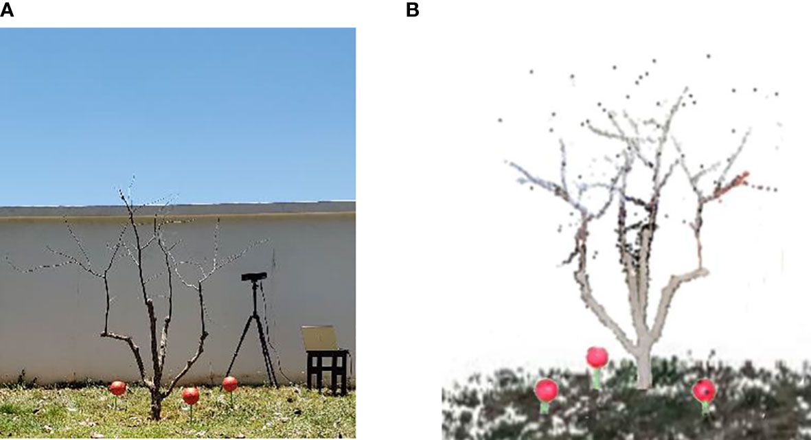
Figure 1 Data acquisition. (A) Experimental scene. (B) Original color point cloud image on one side.

TABLE 1

Table 1 General specifications of Kinect V2.

3. Reconstruction of the dormant jujube tree

3.1. Point cloud preprocessing

Point cloud images obtained by the information acquisition system included ground point clouds, background noise, and outlier noise, so it was necessary to preprocess the original point cloud to obtain the point cloud information of a single jujube tree. According to the 3D point cloud coordinate information of jujube trees, by setting the distance threshold of the 3D point cloud of jujube trees, the point cloud less than the threshold was regarded as the inner point, and the point cloud of jujube trees outside the threshold was removed as the invalid point so as to remove the ground point cloud and background noise to obtain the point cloud of a single jujube tree. The outliers distributed around the branches of jujube trees were filtered by Statistical Outlier Removal (Runions et al., 2005). In the algorithm, parameter λ was the scaling factor, which was determined according to the point cloud density, and the empirical value was [0, 1]. The parameter k was the number of neighbors. In the process of parameter selection, excessive noise removal occurred in Figures 2A, C, and some branches were treated as noise removal. In Figure 2B, some noise was not removed. The best denoising effect is shown in Figure 2D.

FIGURE 2

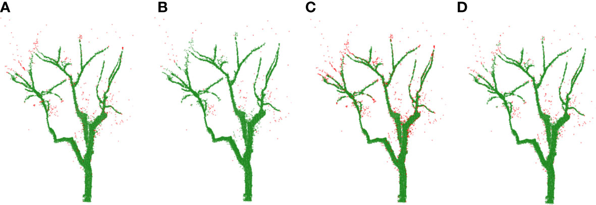
Figure 2 Comparisons of removing noise (noise is shown in red color). (A) k = 30, λ = 0.2. (B) k = 30, λ = 0.5. (C) k = 40, λ = 0.2. (D) k = 40, λ = 0.5.

3.2. Reconstruction pipeline

Point cloud data obtained under one-sided vision could not present the complete shape of jujube trees due to partial point cloud loss due to the occlusion between branches. The point clouds on both sides were registered through the information collection of two stations to make up for the lack of local point clouds under a single view (Geng et al., 2015). The Iterative Closest Point (ICP) algorithm (Besl and McKay, 1992) was widely used in the registration of images and point clouds. The registration process could be well completed when the spatial positions of the point clouds on both sides were close or the overlapping area was large, but the registration stability was poor when the point cloud positions were far away, and it was easy to fall into local optimization. The overall three-dimensional reconstruction process is described in Figure 3. First, the sphere centers of target balls in point clouds on both sides were extracted, and the transformation matrix R_i was calculated based on the triangle similarity principle. The initial registration of point clouds on both sides was completed to make them close in space. The curvature of the point cloud was calculated based on the initial registration point cloud, and then the point pairs with similar curvature were searched. Finally, the ICP algorithm was used to obtain the transformation matrix R_f to achieve fine registration. More details about the methods and algorithms used in the 3D reconstruction of dormant jujube trees were available in previous work (Fu et al., 2020).

FIGURE 3

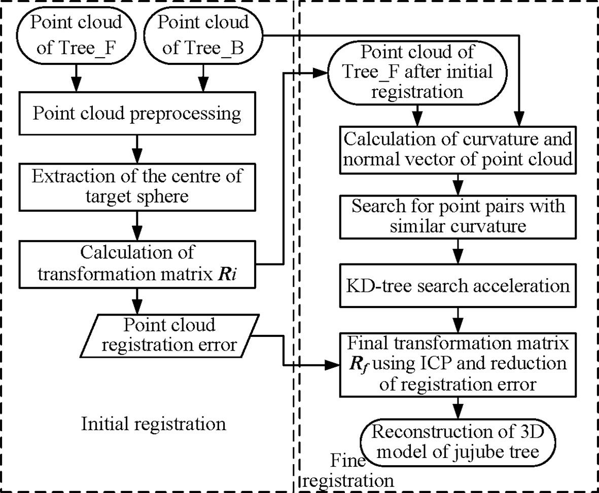
Figure 3 The overall reconstruction pipeline.

4. Skeletonization based on space colonization algorithm

The reconstructed point cloud model had a large amount of data and insignificant features, which is not conducive to tree structure analysis. It was necessary to transform the point cloud into a form that was easy to process so as to reduce information redundancy. The space colonization algorithm (Runions et al., 2005) was based on the principle of space competition for plant growth. The skeleton generated a tree-like structure by continuously competing for the growth space, which made the point cloud model into manageable skeleton data. In the process of skeleton generation, the neighboring space points of skeleton points influence the skeleton trend to be formed. The skeleton expanded continuously with the generation of skeleton points until the algorithm ended when no neighboring space points influenced the skeleton. Figure 4 shows the skeleton generation process of the space colonization algorithm.

FIGURE 4

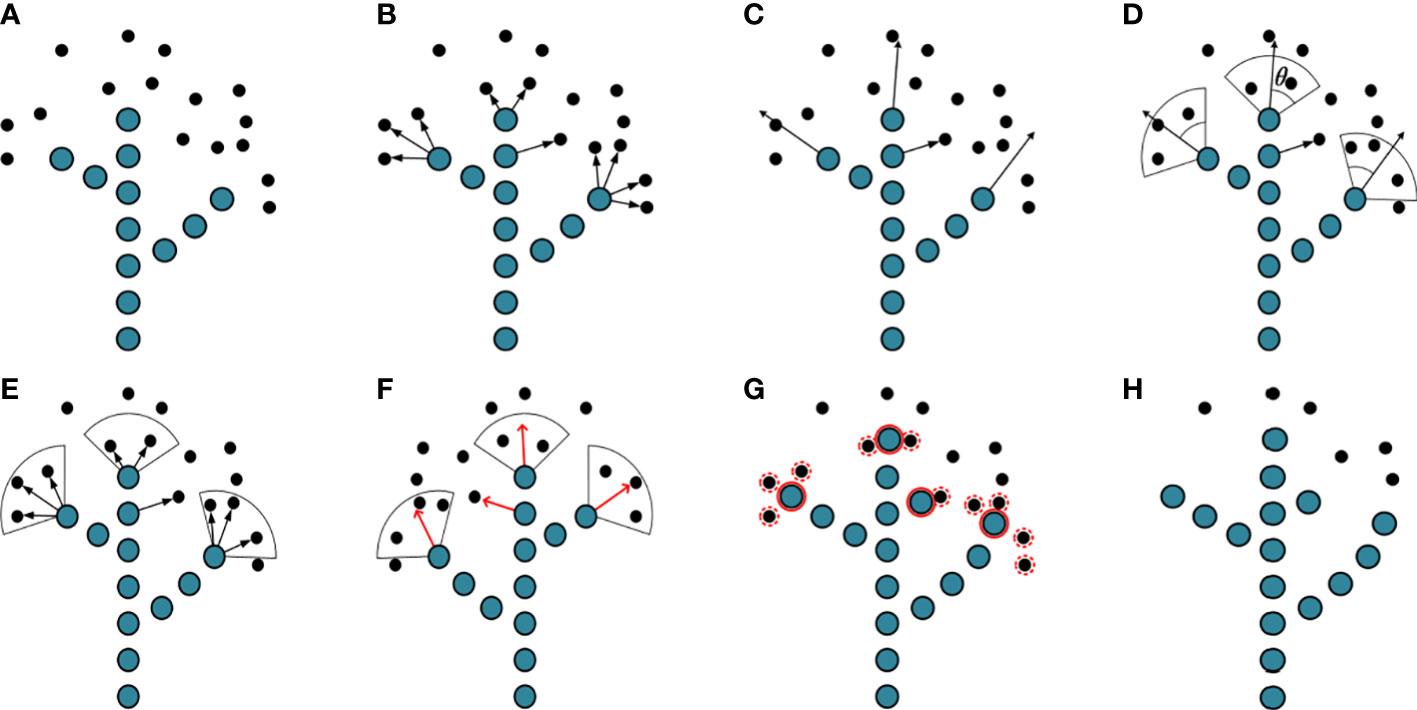
Figure 4 Illustration of space colonization algorithm. (A) Skeleton points and space points. (B) Connect the skeleton point with its space points. (C) Estimate neighborhood directions. (D) Calculate growth neighborhood. (E) Connect space points within growth neighborhoods. (F) Calculating growth vectors. (G) Generate new skeleton points and delete space points. (H) Complete an iteration.

1) In Figure 4A, the current skeleton is composed of 13 blue skeleton points. There are 16 black space points q waiting to be searched globally to influence the skeleton trend. Initialize the tree skeleton array to store the tree skeleton coordinates. Assume that the search radius of the skeleton point p is R, and the space points q within the search radius are stored in set S(p). One space point q affects only the nearest skeleton point p, while the skeleton point p is affected by multiple space points within the search radius. The mathematical relationship between the skeleton point p and the space point in set S(p) is shown in Eq. (1).

$\begin{array}{ll}\{\begin{array}{l}\left|q-p\right|<R\\ \left|p-q\right|=\min \left\{\left|p-q_x\right|,q_x\in S\left(p\right)\right\}\end{array}& (1)\end{array}$

where q is the space point within the search radius R of the skeleton point p. q_x is the serial number of space point q in x sets.

2) Estimate neighborhood directions. Connect the skeleton point with its space points in set S(p) as shown in Figure 4B. Calculate the direction vector, and use the sum of the direction vectors as the direction vector V_p of the neighborhood, as shown by the black arrow in Figure 4C. V_p is calculated by Eq. (2).

$\begin{array}{ll}{V}_p={\displaystyle \sum _{p\in S\left(p\right)}\frac{p-q}{\Vert p-q\Vert }}& (2)\end{array}$

3) The neighborhood range is determined by the direction vector of the neighborhood. The growth neighborhood is a sector area with an angle of 2θ and a sector radius of R. The space points belonging to the neighborhood in set S(p) are calculated by Eq. (3). The space points belonging to the neighborhood are shown in Figure 4D.

$\begin{array}{ll}\arccos \left(V_{pq}·V_p\right)\le \theta & (3)\end{array}$

where V_pq is the vector pq.

4) Calculate the direction of child skeleton points generated by the current skeleton point (parent skeleton point). Connect the skeleton point to multiple space points in its growth neighborhood and calculate their respective vectors (vector direction from skeleton point to space point), as shown by the black arrow in Figure 4E. Take the direction of the vector sum as the growth direction of the skeleton and normalize its value, as shown by the red arrow in Figure 4F. The specific mathematical relationship is shown in Eq. (4).

$\begin{array}{ll}\{{}_{f=\frac{F}{\Vert F\Vert }}^{F={\displaystyle \sum _{p\in S\left(p\right)}\frac{p-q}{\Vert p-q\Vert }}}& (4)\end{array}$

where F is the sum of vectors; f is the sum of normalized vectors.

5) The space distance between the skeleton point and the child skeleton point generated is D_s. The position P_i of the new skeleton point is calculated by Eq. (5).

$\begin{array}{ll}{P}_i=D_s\times f& (5)\end{array}$

6) The respective Euclidean distances between the child skeleton point and space points are calculated by Eq. (6). If the distance is less than the preset deletion threshold R_d, the space point is deleted. The red solid circles are the child skeleton points participating in the calculation, and the red dashed circles are space points to be deleted, as shown in Figure 4G. In one iteration of the algorithm, two primary branches are expanded, the trunk grows upwards, and a new primary branch is formed, as shown in Figure 4H.

$\begin{array}{ll}\left|q-P_i\right|\le R_d& (6)\end{array}$

The space colonization algorithm took the reconstructed point cloud of a jujube tree as input and then iteratively generated the skeleton, as shown in Figure 5. The skeleton was a tree-like structure that reflected the topology of jujube trees. The skeleton point data were stored in the child linked list structure, and each parent skeleton point can query the generated child skeleton points.

FIGURE 5

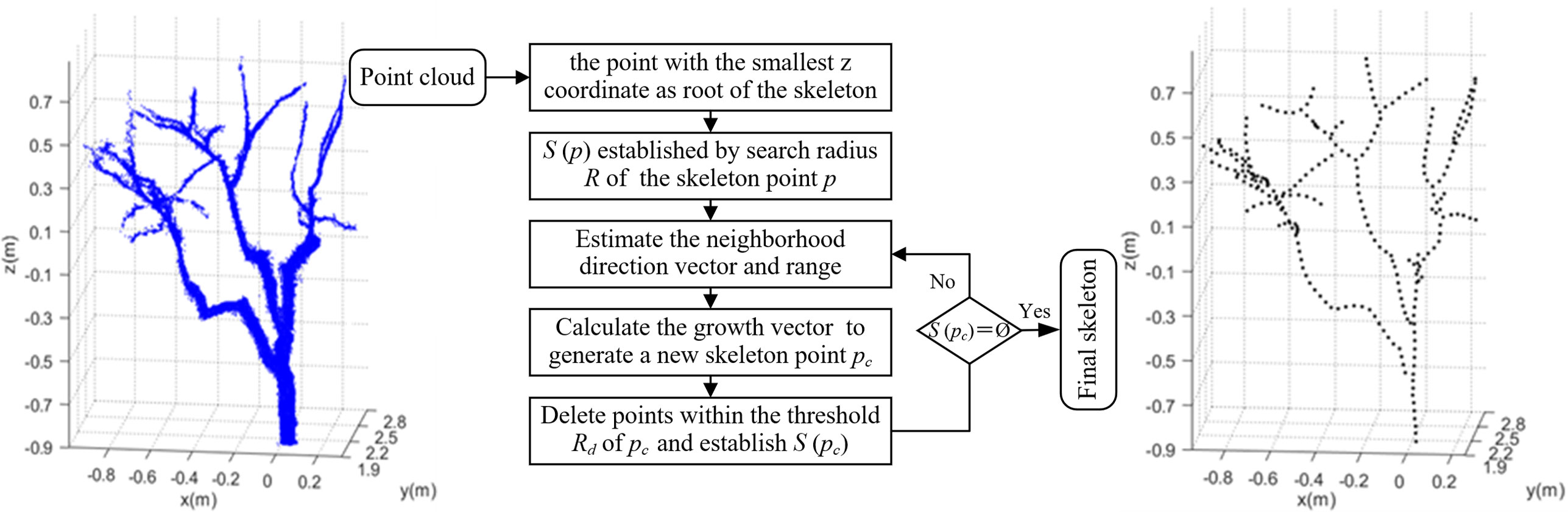
Figure 5 Flowchart of skeletonization using space colonization algorithm.

5. Skeleton analysis and modeling

5.1. Trunk and primary branch identification

According to the generation relationship between skeleton points, the parent skeleton point connected its child skeleton points to form a directed graph G(C,E), and the direction was from the parent skeleton point to the child skeleton point, where $C={\left\{c_i\right\}}_{i=1}^{N_c}$ was the vertex set; that is, all skeleton points and E = {(c_i, c_k)} were the set of edges between connected skeleton points.

After the directed graph G (C, E) was established, we needed to identify the subgraph G_T (C_T, E_T) that corresponded to skeleton points that belong to the trunk. Since we knew that the trunk of the tree began close to the ground and followed an approximately vertical trajectory, we identified G_T according to the following heuristics. Assume that initially C_T = Ø and E_T = Ø. The edge e_i was the successor edge of e_s. e_i = {(a,b)|a = c_i, and (a,b)∈E} was the set of edges in E that includes c_i as one of its vertices. The beginning edge of the trunk was formed by the root skeleton point c_i with the smallest z coordinate and its child skeleton points. Subsequently, the successor edges and the successor vertices were searched from the beginning edge. If e_i was the only successor edge of e_s, the edge e_i = (c_i, c_k) was directly added to E_T. When there were multiple successor edges, the change angle of e_i relative to e_s was calculated by Eqs (7) and (8) to determine the unique successor edge e_i.

$\begin{array}{ll}\psi (\overrightarrow{e_i},\overrightarrow{e_s})={\cos }^{-1}\left(\frac{\overrightarrow{e_i}·\overrightarrow{e_s}}{\Vert \overrightarrow{e_i}\Vert \Vert \overrightarrow{e_s}\Vert }\right)& (7)\end{array}$

$\begin{array}{ll}{e}_i^{\ast }=\arg \min \left[\psi \left(\overrightarrow{e_i},\overrightarrow{e_s}\right)\right]& (8)\end{array}$

where $e_i^{\ast }$ corresponds to the successor edge that showed the smallest change angle relative to e_s in e_i. If ψ was within the threshold, $e_i^{\ast }$ = (c_i, c_k) was added to E_T, and c_i and c_k were added to C_T. Restart the procedure from c_k, and terminate it when ψ exceeded the threshold. This approach guaranteed that the algorithm did not continue to search toward the primary branch at the top of the trunk. The green edges in Figure 6A show the result of the trunk detection algorithm.

FIGURE 6

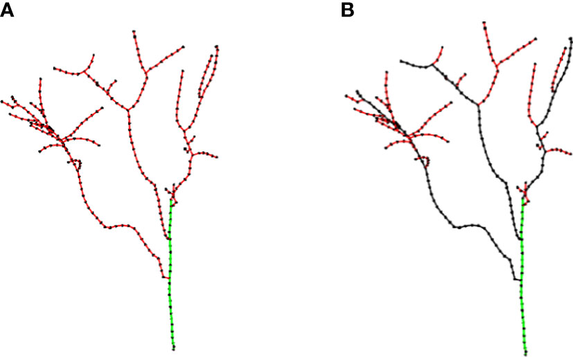
Figure 6 Results of skeleton analysis. (A) Trunk (green edges). (B) Primary branches (black edges).

Primary branches G_B (C_B, E_B) were identified on the basis of trunk G_T (C_T, E_T). The beginning point of the primary branch was the point belonging to the trunk, which was the vertex of the trunk with multiple edges or at the top of the trunk. For the convenience of description, the beginning points of the two types were collectively called PB_start. After the trunk was identified, a depth-first search was used to find primary branches, as follows.

(1) Mark a beginning point PB_start as the current point, and search the successor vertices of the current point as candidate points.

(2) Find an adjacent point not marked as a trunk among candidate points and mark the new point as the current point.

(3) The depth-first search is performed on the subgraph with the current point as the root node in the directed graph, and the vertices without successor points in the access process are marked as the endpoints.

(4) Trace back from the endpoint to the starting point PB_start and calculate the sum of Euclidean distances L_i between all the points in each backtracking path.

(5) Mark the path with the highest cumulative Euclidean distances as the primary branch beginning from PB_start. Repeat steps 1 through step 5 until all primary branches are identified.

Figure 6B shows the final result of primary branch identification. The black edges were primary branches identified, and the remaining red edges were lateral branches.

5.2. Pruning point identification

During the dormancy period, the managers cut off the end of the primary branch, which accounted for about 1/3 of the length of the primary branch. Pruning was helpful to reduce nutrient consumption in the dormancy period and make nutrient supply concentrated in the middle of main branches to cultivate fruiting branch groups so as to fully improve the production potential of jujube trees. Pruning rules, while simple, could greatly increase efficiency in seasonal pruning. Therefore, the length of the primary branch became the key parameter in the pruning point identification algorithm. In this study, the pruning length of the primary branch was not set to a fixed value but to an adaptive length, which located the pruning point at 2/3L_i from the beginning point of the primary branch. The pink dots are the identified pruning points, as shown in Figure 7.

FIGURE 7

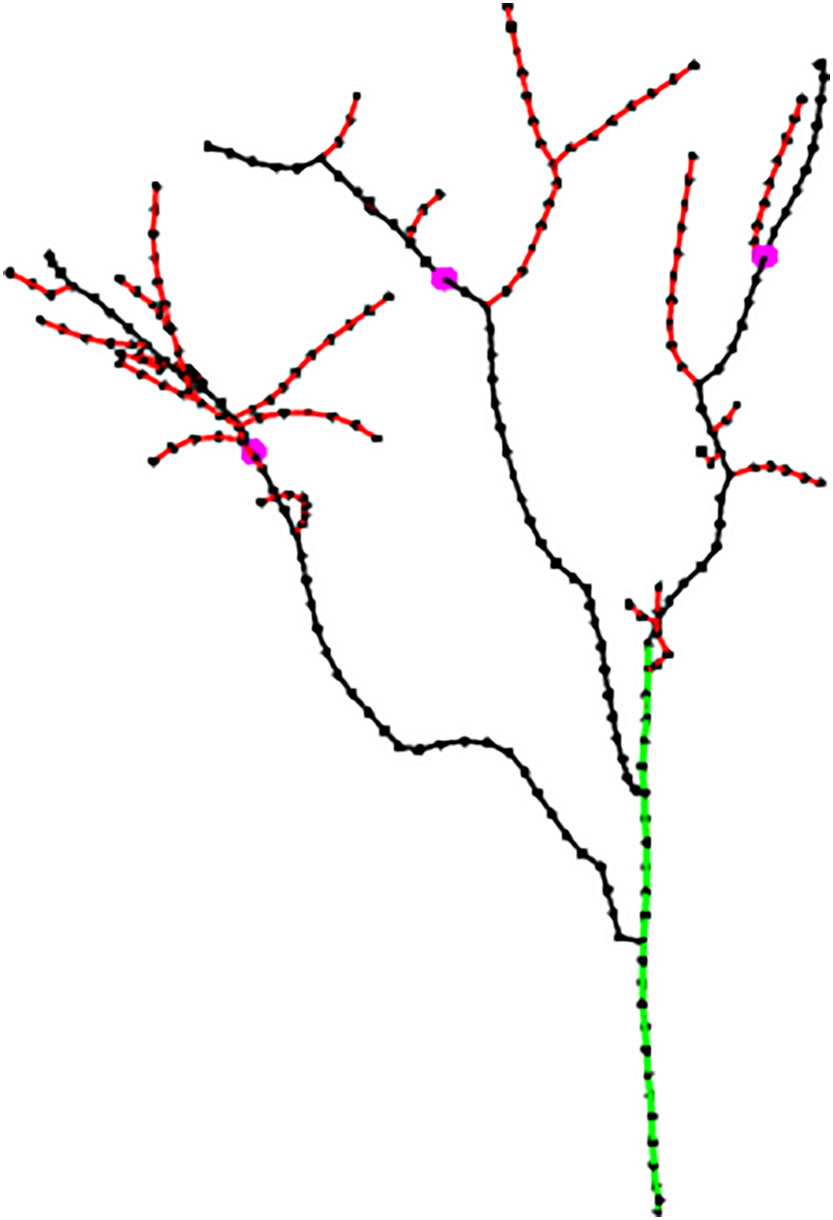
Figure 7 Identification results of pruning points (pink dots) on primary branches.

5.3. Modeling

To visualize the pruned jujube trees, the model was based on the pruned skeleton. The trunk of jujube trees was Grade 1 branch, the primary branches were Grade 2 branches, and the remaining branches were Grade 3 branches. The branch thickness gradually decreased from Grade 1 to Grade 3. The change of branch thickness followed the rule of gradually thinning from the beginning to the end. After the determination of the pruned skeleton information, the geometric model of the trunk and primary branches was represented by a multi-segment cylindrical connection. The edges in the directed graph were set as the center axis of the cylinder, as shown in Figure 8. However, the two base radii of the cylinder, that is, the thickness of the branch, have not been determined. The pipeline model theory was widely used in estimating branch thickness (Shi et al., 2019). The thickness of the parent branch and the generated child branches was calculated by Eq. (9).

FIGURE 8

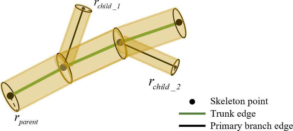
Figure 8 Schematic diagram of branch modeling.

$\begin{array}{ll}{r}_{parent}^n={\displaystyle \sum _{i=1}^m{r}_{child\_i}^n}& (9)\end{array}$

where r_parent is the beginning radius of the parent branch, r_{child_i} is the beginning radius of the child branch, m is the number of child branches, and n is generally taken as 2. The root of the jujube tree was measured, and the beginning radius of all branches was calculated from the root. According to the pruned skeleton and radius, the cylinder was continuously generated along the skeleton trend to build a geometric model.

6. Results and analysis

6.1. Comparative analysis of point cloud registration errors

To verify the stability of the individual reconstruction algorithm proposed in this study, 15 jujube trees were registered, and the results are shown in Figure 9. It could be seen that the registration errors were less than 0.91 cm, and the average registration error was 0.66 cm. The optimized ICP algorithm greatly improved the accuracy of point cloud registration. The comparison results show that the algorithm proposed in this study has high stability and reliability and meets the application requirements of a reconstructed jujube point cloud.

FIGURE 9

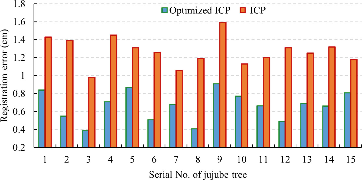
Figure 9 Comparison of point cloud registration errors.

6.2. Skeleton extraction and pruning point identification

The point cloud of jujube trees collected in the field was reconstructed to obtain complete point cloud information on jujube trees, and the Alpha-shape algorithm was used to triangulate the point cloud to improve the visual effect of the jujube tree model. The jujube tree individual model is shown in Figure 10A. A space colonization algorithm was used to extract the jujube tree skeleton with a search radius R of 8.2 cm, a growth neighborhood θ of 22.5°, a skeleton point spacing D_s of 4.0 cm, and a deletion threshold R_d of 6.0 cm. Figure 10B shows the skeleton generated by the space colonization algorithm, trunk and primary branches identified by the skeleton analysis algorithm, and pruning points located by the pruning rule. The number of beginning points PB_start determined by the skeleton analysis algorithm in Tree 1 was four, of which three were the inner points of the trunk and one was the top endpoint of the trunk. Each inner point generated one primary branch, and the top point generated two primary branches. The red edge marked was the false primary branch because this beginning point was close to the bifurcation of two primary branches, and there was local noise at the same time, which resulted in unreasonable branches when the space colonization algorithm generated the skeleton. The red edge marked in Tree 3 has stopped growing due to necrosis, and its length was short, which did not meet the requirements of pruning. It was also one of the false primary branches. In order to improve the robustness of the algorithm to the identification of primary branches, the minimum length of primary branches was set to 50 cm so as to avoid adding false branches such as unreasonable branches or short branches to the primary branches G_B (C_B, E_B). After the length threshold setting, the global skeleton was marked as the trunk (green edges), primary branches (black edges), and lateral branches (red edges) by the algorithm. Finally, pruning points (pink dots) of primary branches were identified under the guidance of the pruning rule.

FIGURE 10

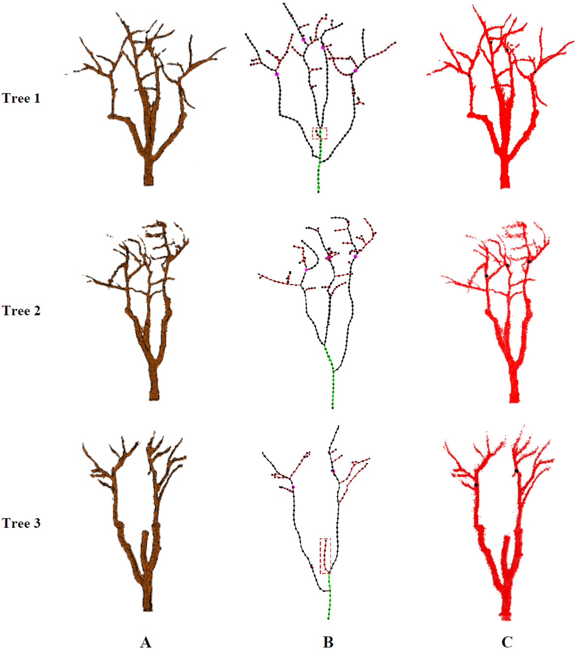
Figure 10 Results of skeleton analysis and pruning points identification. (A) Model of jujube tree. (B) Identification of pruning points based on skeleton analysis. (C) Mapping of pruning point positions in reconstructed point cloud.

In order to evaluate the reliability of the pruning point information and ensure that the robot could achieve the pruning operation according to the pruning points, the three-dimensional coordinate information of the pruning points was mapped in the reconstructed point cloud. Pruning point information in Figure 10C was located on the primary branches, which showed that the identified pruning point information was effective, and also verified that the skeleton extracted by the space colonization algorithm had a high degree of coincidence with the three-dimensional structure of jujube trees.

6.3. Modeling

Branch modeling could predict the shape of jujube trees after pruning in advance so as to avoid irreversible operations such as incorrect pruning. According to the actual pruning operation, the pruned branch was partially removed from the tree, that is, all skeleton points in the skeleton generated by the pruning point were deleted. The root radii of Tree 1, Tree 2, and Tree 3 were measured at 4.1, 3.4, and 4.0 cm, respectively. The beginning radius of all branches was calculated from the root. The roughness of the beginning of all branches was calculated from the bottom to the top of the root, and the visualization of the pruned jujube tree was achieved by combining the central axis information of the pruned skeleton (Figure 11).

FIGURE 11

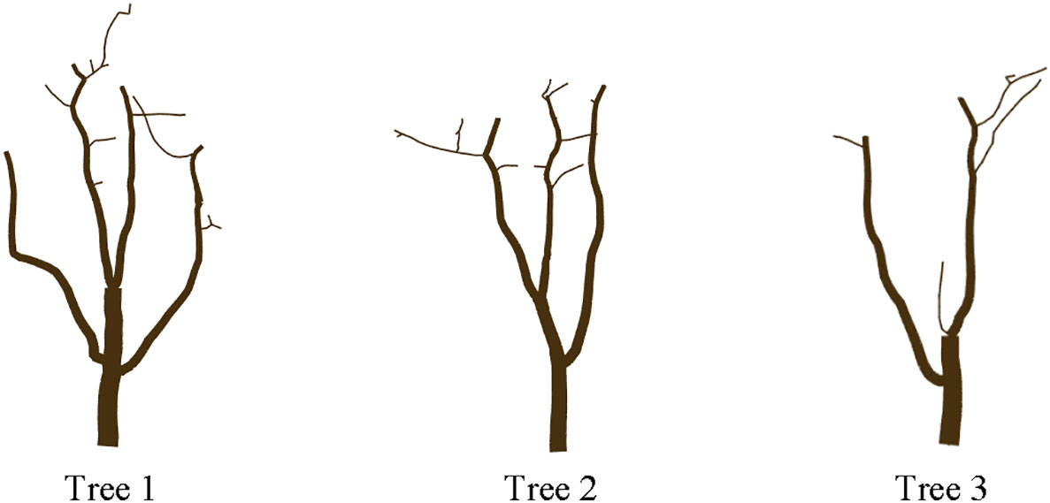
Figure 11 Model of jujube tree after pruning.

7. Discussion

The final shape of the tree skeleton depended on four parameters for search radius, growth neighborhood, skeleton point spacing, and deletion threshold of the space colonization algorithm. In the process of skeleton generation by the algorithm, the skeleton of the trunk and primary branches best matched the tree shape as shown in the black box (Figure 12). The skeleton at the bifurcation of the primary branch and the lateral branch in the red box deviated from the point cloud but returned to normal quickly. This was because when the space colonization algorithm iteratively generated the lateral branch, the search radius contained more point clouds of the primary branch, which interfered with the skeleton generation of the lateral branch. However, as the distance between the lateral branch and the primary branch increased, the number of point clouds belonging to the primary branch decreased. Subsequently, the influence of the primary branch was weakened, and finally, the lateral branch skeleton returned to normal and coincides with the tree shape.

FIGURE 12

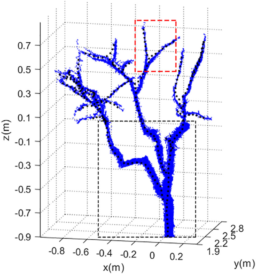
Figure 12 Point cloud of jujube tree (blue) and its skeleton (black).

The search radius of the algorithm was robust when generating trunk and primary branches. However, for the lateral branches, if the search radius was too large, it would be easily affected by primary branches. Therefore, when formulating the pruning rule, pruning points were not determined by the fixed pruning length but selected 1/3 of the distance from the end of the primary branch to avoid the place where the side branches were dense as far as possible and located pruning points in the robust area of the skeleton. In the next work, the adaptability of parameters should be improved. With the change in branch density, the search radius and deletion threshold should be appropriately increased or reduced to further improve the similarity between skeleton and tree shape and ensure the effectiveness of identifying pruning points.

8. Conclusions

In this study, a low-cost depth camera was used to collect point cloud data on both sides of jujube trees. The point cloud data were preprocessed to remove noise. Point cloud registration was conducted by combining manual marking with an optimized ICP algorithm to achieve the reconstruction of jujube individual information. The registration errors were less than 0.91 cm, and the average registration error was 0.66 cm, which provided good individual data for the skeleton generation of the space colonization algorithm. Triangulate the reconstructed point cloud with the Alpha-shape algorithm, which could make the model more similar to the real tree in appearance, and was the visual basis for the automatic pruning of jujube trees.

The space colonization algorithm generated the skeleton reflecting the topological structure of the jujube tree by iteration. A directed graph was constructed using skeleton points to represent the tree structure and the parent–child relationship between skeleton points. According to the tree structure and the characteristics of the directed graph of jujube trees, the skeleton was analyzed to identify the trunk and primary branches. The branch length threshold solved the problem of false primary branches in the skeleton. Subsequently, under the guidance of the pruning rule, the pruning points were identified, and the validity of the pruning points was verified by using the information mapping method. Finally, the visual model was constructed based on the remaining skeleton information to realize the appearance of the pruned tree.

Primary branches of jujube trees identified by the algorithm might deviate from the result of our actual judgment because the branch length obtained by the depth-first search was the only factor for primary branch identification. In the next step, we will take into account both the length of the main branch and the angle change of the main branch at the branch bifurcation and add appropriate weights to these two factors. We will sort the possible primary branches originating at the same point through the scoring principle so that the results of the algorithm are more consistent with human judgment.

Data availability statement

The original contributions presented in the study are included in the article/supplementary material. Further inquiries can be directed to the corresponding authors.

Author contributions

YF designed and performed the experiment, selected the algorithms, analyzed the data, debugged the algorithms, and wrote the manuscript. YF, YX, MF, YW, and CS collected the data. HZ monitored the data analysis. WF and HZ conceived the study and participated in its design. All authors contributed to this article and approved the submitted version.

Funding

This work was supported by the Key R&D Projects in Hainan Province (Grant No. ZDYF2022XDNY231), the National Natural Science Foundation of China (Grant No. 52265040), and the National Natural Science Foundation of China (Grant No. 51765058).

Acknowledgments

The authors would like to thank their schools and colleges, as well as the funding of the project. All support and assistance are sincerely appreciated. Additionally, the authors sincerely appreciate the work of the editor and the reviewers of the present paper.

Conflict of interest

The authors declare that the research was conducted in the absence of any commercial or financial relationships that could be construed as a potential conflict of interest.

Publisher’s note

All claims expressed in this article are solely those of the authors and do not necessarily represent those of their affiliated organizations, or those of the publisher, the editors and the reviewers. Any product that may be evaluated in this article, or claim that may be made by its manufacturer, is not guaranteed or endorsed by the publisher.

References

Adhikari, B., Karkee, M. (2011). 3D reconstruction of apple trees for mechanical pruning. ASABE Annu. Int. Meet; 2011 August 7 - August 10; Louisville, Kentucky. doi: 10.13031/2013.38139

CrossRef Full Text | Google Scholar

Besl, P. J., McKay, N. D. (1992). A method for registration of 3-d shapes. IEEE Trans. Pattern Anal. Mach. Intell. 14 (2), 239–256. doi: 10.1109/34.121791

CrossRef Full Text | Google Scholar

Botterill, T., Paulin, S., Green, R., Williams, S., Lin, J., Saxton, V., et al. (2017). A robot system for pruning grape vines. J. Field Rob. 34 (6), 1100–1122. doi: 10.1002/rob.21680

CrossRef Full Text | Google Scholar

Crassweller, R., Peter, K., Krawczyk, G., Schupp, J., Ford, T., Brittingham, M., et al. (2020). 2020-21 Penn state tree fruit production guide. Penn. State Extension Publ. AGRS-045 446.

Google Scholar

Díaz, C. A., Pérez, D. S., Miatello, H., Bromberg, F. (2018). Grapevine buds detection and localization in 3D space based on structure from motion and 2D image classification. Comput. Ind. 99, 303–312. doi: 10.1016/j.compind.2018.03.033

CrossRef Full Text | Google Scholar

Digumarti, S. T., Nieto, J., Cadena, C., Siegwart, R., Beardsley, P. (2018). Automatic segmentation of tree structure from point cloud data. IEEE Robot. Autom. Lett. 3 (4), 3043–3050. doi: 10.1109/LRA.2018.2849499

CrossRef Full Text | Google Scholar

Elfiky, N. M., Akbar, S. A., Sun, J., Park, J., Kak, A. (2015). “Automation of dormant pruning in specialty crop production: an adaptive framework for automatic reconstruction and modeling of apple trees,” in: 2015 IEEE Computer Society Conference on Computer Vision and Pattern Recognition Workshops (Boston, MA, USA: IEEE). 65–73.

Google Scholar

Fernandes, M., Scaldaferri, A., Fiameni, G., Teng, T., Gatti, M., Poni, S., et al. (2021). “Grapevine winter pruning automation: on potential pruning points detection through 2d plant modeling using grapevine segmentation,” in: 2021 IEEE 11th Annual International Conference on CYBER Technology in Automation, Control, and Intelligent Systems (CYBER) (Jiaxing, China: IEEE). 13–18.

Google Scholar

Fu, Y., Li, C., Zhu, J., Wang, B., Zhang, B., Fu, W. (2020). Three-dimensional model construction method and experiment of jujube tree point cloud using alpha-shape algorithm. Trans. Chin. Soc Agric. Eng. 36 (22), 214–221. doi: 10.11975/j.issn.1002-6819.2020.22.024

CrossRef Full Text | Google Scholar

Geng, N., Ma, F., Yang, H., Li, B., Zhang, Z. (2015). Neighboring constraint-based pairwise point cloud registration algorithm. Multimed. Tools Appl. 75 (24), 16763–16780. doi: 10.1007/s11042-015-2941-6

CrossRef Full Text | Google Scholar

He, L., Schupp, J. (2018). Sensing and automation in pruning of apple trees: a review. Agronomy 8 (10), 211. doi: 10.3390/agronomy8100211

CrossRef Full Text | Google Scholar

Karkee, M., Adhikari, B. (2015). A method for three-dimensional reconstruction of apple trees for automated pruning. Trans. ASABE. 58 (3), 565–574. doi: 10.13031/trans.58.10799

CrossRef Full Text | Google Scholar

Karkee, M., Adhikari, B., Amatya, S., Zhang, Q. (2014). Identification of pruning branches in tall spindle apple trees for automated pruning. comput. Electron. Agric. 103, 127–135. doi: 10.1016/j.compag.2014.02.013

CrossRef Full Text | Google Scholar

Kolmanič, S., Strnad, D., Kohek, Š., Benes, B., Hirst, P., Žalik, B. (2021). An algorithm for automatic dormant tree pruning. Appl. Soft Comput. 99, 106931. doi: 10.1016/j.asoc.2020.106931

CrossRef Full Text | Google Scholar

Lin, G., Tang, Y., Zou, X., Wang, C. (2021). Three-dimensional reconstruction of guava fruits and branches using instance segmentation and geometry analysis. Comput. Electron. Agric. 184, 106107. doi: 10.1016/j.compag.2021.106107

CrossRef Full Text | Google Scholar

Ma, B., Yan, J., Wang, L., Jiang, H. (2021a). Three-dimensional point cloud automatic registration for dwarf and dense planted jujube tree based on skeleton points. Trans. Chin. Soc Agric. Mach. (Huangshan, China: IEEE) 52, 24–32. doi: 10.6041/j.issn.1000-1298.2021.09.003

CrossRef Full Text | Google Scholar

Ma, B., Yan, J., Wang, L., Jiang, H. (2021b). Automatic branch detection of jujube trees based on 3D reconstruction for dormant pruning using the deep learning-based method. Comput. Electron. Agric. 190, 106484. doi: 10.1016/j.compag.2021.106484

CrossRef Full Text | Google Scholar

Majeed, Y., Zhang, J., Zhang, X., Fu, L., Karkee, M., Zhang, Q., et al. (2020). Deep learning based segmentation for automated training of apple trees on trellis wires. Comput. Electron. Agric. 170, 105277. doi: 10.1016/j.compag.2020.105277

CrossRef Full Text | Google Scholar

Medeiros, H., Kim, D., Sun, J., Seshadri, H., Akbar, S. A., Elfiky, N. M., et al. (2017). Modeling dormant fruit trees for agricultural automation. J. Field Rob. 34 (7), 1203–1224. doi: 10.1002/rob.21679

CrossRef Full Text | Google Scholar

Mika, A., Buler, Z., Treder, W. (2016). Mechanical pruning of apple trees as an alternative to manual pruning. Acta Sci. Pol. Hortorum Cultus. 15 (1), 113–121.

Google Scholar

Runions, A., Fuhrer, M., Lane, B., Federl, P., Rolland-Lagan, A. G., Prusinkiewicz, P. (2005). Modeling and visualization of leaf venation patterns. ACM Trans. Graph. 24 (3), 702–711.

Google Scholar

Shi, Y., Geng, N., Hu, S., Zhang, Z., Zhang, J. (2019). Illumination distribution model of apple tree canopy based on random forest regression algorithm. Trans.Chinese Soc Agric. Mach. 50 (5), 214–222. doi: 10.6041/j.issn.1000-1298.2019.05.025

CrossRef Full Text | Google Scholar

Tang, Y., Zhou, H., Wang, H., Zhang, Y. (2023). Fruit detection and positioning technology for a camellia oleifera c. Abel orchard based on improved YOLOv4-tiny model and binocular stereo vision. Expert Syst. Appl. 211, 118573. doi: 10.1016/j.eswa.2022.118573

CrossRef Full Text | Google Scholar

Wang, H., Lin, Y., Xu, X., Chen, Z., Wu, Z., Tang, Y. (2022). A study on long-close distance coordination control strategy for litchi picking. Agronomy 12 (7), 1520. doi: 10.3390/agronomy12071520

CrossRef Full Text | Google Scholar

Yang, L., Zhang, L., Dong, H., Alelaiwi, A., Saddik, A. E. (2015). Evaluating and improving the depth accuracy of kinect for windows v2. IEEE Sens. J. 15 (8), 4275–4285. doi: 10.1109/JSEN.2015.2416651

CrossRef Full Text | Google Scholar

Yan, D., Wintz, J., Mourrain, B., Wang, W., Boudon, F., Godin, C. (2009). “Efficient and robust reconstruction of botanical branching structure from laser scanned points,” in: 2009 11th IEEE International Conference on Computer-Aided Design and Computer Graphics. (Huangshan, China: IEEE) 572–575.

Google Scholar

Zahid, A., Mahmud, M. S., He, L., Choi, D., Heinemann, P., Schupp, J. (2020). Development of an integrated 3R end-effector with a cartesian manipulator for pruning apple trees. Comput. Electron. Agric. 179, 105837. doi: 10.1016/j.compag.2020.105837

CrossRef Full Text | Google Scholar

Zahid, A., Mahmud, M. S., He, L., Heinemann, P., Choi, D., Schupp, J. (2021). Technological advancements towards developing a robotic pruner for apple trees: A review. Comput. Electron. Agric. 189, 106383. doi: 10.1016/j.compag.2021.106383

CrossRef Full Text | Google Scholar

Zhang, J., He, L., Karkee, M., Zhang, Q., Zhang, X., Gao, Z. (2018). Branch detection for apple trees trained in fruiting wall architecture using depth features and regions-convolutional neural network (R-CNN). Comput. Electron. Agric. 155, 386–393. doi: 10.1016/j.compag.2018.10.029

CrossRef Full Text | Google Scholar