- 1 Department of Molecular Physiology, Max Planck Institute of Molecular Plant Physiology, Potsdam-Golm, Germany
- 2 Botanical Institute II, University of Cologne, Cologne, Germany
With the development of high-throughput metabolic technologies, a plethora of primary and secondary compounds have been detected in the plant cell. However, there are still major gaps in our understanding of the plant metabolome. This is especially true with regards to the compartmental localization of these identified metabolites. Non-aqueous fractionation (NAF) is a powerful technique for the determination of subcellular metabolite distributions in eukaryotic cells, and it has become the method of choice to analyze the distribution of a large number of metabolites concurrently. However, the NAF technique produces a continuous gradient of metabolite distributions, not discrete assignments. Resolution of these distributions requires computational analyses based on marker molecules to resolve compartmental localizations. In this article we focus on expanding the computational analysis of data derived from NAF. Along with an experimental workflow, we describe the critical steps in NAF experiments and how computational approaches can aid in assessing the quality and robustness of the derived data. For this, we have developed and provide a new version (v1.2) of the BestFit command line tool for calculation and evaluation of subcellular metabolite distributions. Furthermore, using both simulated and experimental data we show the influence on estimated subcellular distributions by modulating important parameters, such as the number of fractions taken or which marker molecule is selected. Finally, we discuss caveats and benefits of NAF analysis in the context of the compartmentalized metabolome.
Introduction
Although the main biochemical pathways in plants have been resolved by classical biochemical approaches in the last century (Fernie, 2007; Stitt et al., 2010a), many aspects of cellular metabolism and its regulatory functions are still not well understood, mostly due to technical limitations in gathering a more holistic insight into the cell’s biochemistry. In recent years tremendous progress has been made in the establishment of high-throughput methods enabling the simultaneous analysis of a multitude of chemically diverse, small molecule metabolites from highly complex compound mixtures (Fiehn, 2001; Kopka et al., 2004; Brown et al., 2005; Pan and Raftery, 2007). Metabolomics, the comprehensive study of an organism’s metabolite composition, has thus become an important tool in functional genomics and systems biology (Fernie et al., 2004; Saito and Matsuda, 2010). It has been widely used to study metabolic responses toward altered gene expression (Junker et al., 2006; Mugford et al., 2009; Albinsky et al., 2010), biotic and abiotic stresses (Kaplan et al., 2004; Bednarek et al., 2009), to characterize genetic and metabolic diversity (Schauer et al., 2006; Huege et al., 2011; Kusano et al., 2011), and has been combined with further Omic technologies in systems biology driven research (Kaplan et al., 2007; Hannah et al., 2010; Jozefczuk et al., 2010). While unexpected findings have yielded refined pathways as well as insights into their regulation and evolution (Zeeman et al., 2004; Eisenhut et al., 2008; Bednarek et al., 2009; Fettke et al., 2009), it has become evident that cellular metabolism needs to be considered as a highly integrative network bridging the genotype and ultimate phenotype or cellular responses (Meyer et al., 2007; Sweetlove et al., 2008; Sulpice et al., 2009; Stitt et al., 2010b). Even though the abovementioned studies provided major breakthroughs in the description of biological systems, we are still lacking information concerning the temporal and especially spatial regulation of the metabolome (Stitt and Fernie, 2003).
It is widely acknowledged that the compartmentalization of metabolism in eukaryotic cells represents a crucial factor for metabolic activity and functionality (Lunn, 2007). Consequently, the interrelation of metabolic networks within and between compartments needs to be deciphered. Whereas the subcellular localization of enzymes can be computationally predicted (Emanuelsson et al., 2000; Schwacke et al., 2003) or experimentally determined (Carter et al., 2004; Heazlewood et al., 2007; Taylor et al., 2011), the analysis of the subcellular localization of metabolites, the products and substrates of these enzymes, is more challenging due to redundant pathways, transport, and storage (Kruger and Von Schaewen, 2003; Büttner, 2007; Rébeillé et al., 2007; Krueger et al., 2010). Further hurdles for reliable metabolite determinations in subcellular compartments are the fast turnover (Stitt et al., 1983; Stitt and Fernie, 2003) and the exceptionally rapid translocation of metabolites between compartments (Bowsher and Tobin, 2001; Martinoia et al., 2007; Weber and Fischer, 2007). Because of this, methods providing accurate information on the subcellular distributions of multiple metabolites are still limited.
Immunohistochemistry has been utilized to analyze the localization of non-protein molecules, such as cell wall polysaccharides and amino acids, permitting the analysis of metabolite compositions in compartments (e.g., Golgi, ER) which are normally not accessible by fractionation methods (Walker et al., 2001). However, dramatic losses of metabolites have been observed during tissue fixation which makes the interpretation of the results sometimes difficult (Peters and Ashley, 1967; Heinrich and Kuschki, 1978; Zechmann et al., 2011). Nuclear magnetic resonance (NMR) spectroscopy facilitates the determination of in vivo metabolite compositions in cells, tissues, and whole plants (Gout et al., 1993, 2000; Libourel et al., 2006). It requires distinct signals for the different compartments, which can be partly achieved by the pH dependency of the chemical shift of some molecules like inorganic phosphate, or organic and amino acids (Bligny and Douce, 2001). Compared to other spectroscopy/spectrometry methods, NMR is relatively insensitive and thus only feasible for metabolites which are highly abundant in the cell (Bligny and Douce, 2001). Genetically encoded molecular biosensors, proteins fused to two variants of the green fluorescent protein displaying conformational changes and fluorescence resonance energy transfer when a specific ligand binds, represent a promising molecular tool for temporal and spatial analyses of in vivo metabolite dynamics (Fehr et al., 2002; Lalonde et al., 2005; Chen et al., 2010). While this has been successfully applied for subcellular analysis of glucose and glutathione redox potentials (Deuschle et al., 2006; Gutscher et al., 2008), each targeted metabolite requires a unique sensor and therefore only a small number of metabolites might be simultaneously detectable in the same individual transgenic. Another widely used technique is protoplast fractionation. It is based on the fast purification of intact organelles through silicone oil or membrane filters followed by rapid quenching of metabolism (Wirtz et al., 1980; Lilley et al., 1982; Stitt et al., 1989). This method facilitates fractionation of plastids, mitochondria, and the cytosol from a single cell type, commonly mesophyll cells. However, digestion of the cell wall and the purification of protoplasts might substantially affect the metabolic state and therefore the obtained metabolite readout and the transferability of results.
Non-aqueous fractionation (NAF) is probably the most widely used technique to study metabolite compartmentalization, especially in plant science (Gerhardt and Heldt, 1984; Riens et al., 1991; Farre et al., 2001; Fettke et al., 2005; Krueger et al., 2009; Yamada et al., 2009). It separates fragments of subcellular compartments under non-aqueous conditions where biological activities, such as metabolite leakage, conversion, and translocation, are essentially completely arrested (Gerhardt and Heldt, 1984). Small subcellular particles, generated during lyophilization and ultrasonication of ground material, are separated by their composition-dependent density using equilibrium centrifugation in a gradient consisting of two differently dense, non-aqueous solvents (for details see Krueger et al., 2011). The abundance of metabolites and compartment-specific markers, which are also used as anchors to computationally estimate subcellular metabolite distributions, are analyzed throughout the collected gradient fractions. As non-aqueous fractionated material can be combined with a wide range of Omic technologies, it allows the determination of subcellular localizations for a large number of molecules including metabolites and lipids (Farre et al., 2001; Weise et al., 2004; Fettke et al., 2006; Krueger et al., 2011). In its routine application, the NAF technique allows for the separation of three distinct compartments – the cytosol, the plastids, and the vacuole (Riens et al., 1991; Farre et al., 2008; Krueger et al., 2009). However, it was recently shown that the resolution power of this technique has not yet been fully explored (Krueger et al., 2011).
As NAF results in continuous compartmental distributions due to variable and composition-dependent particle densities, computational methods need to be employed to analyze the obtained data. This and the interpretation of generated computational results reflect the main challenges for experimentalists. From the computational point of view as well, this type of data analysis is mostly underexplored.
Using both experimentally derived and simulated data, we investigated the effects of computationally modulating parameters important for the analysis of NAF gradients in order to address several technically and biologically relevant questions, such as: How many fractions are required to produce a good compartmental separation? Does the fraction number or the marker choice influence the estimated compartmental abundances? How good must the compartmental separation be in order to get reasonable estimates of compartmental abundances? How accurate must an estimate of compartmental abundances be in order to be considered valid? Taken together, the answers to these questions give a solid theoretical basis for the planning and execution of NAF experiments. Finally, we demonstrate and discuss alternative visualizations of NAF derived data in order to efficiently integrate additional knowledge to aid in the biological interpretation of the obtained results.
Materials and Methods
The following sections introduce computational terminologies, used throughout the manuscript, denoted as italicized text along with their definition and/or abbreviation.
Experimental Data
Experimental data and associated classifications used in this study were taken from Krueger et al. (2011). In brief, Arabidopsis thaliana leaf material was harvested 3 h after the onset of light and separated using an optimized NAF protocol (Krueger et al., 2009, 2011). A total of six fractions from three independent gradients were analyzed using mass-spectrometry (MS) – based metabolite profiling for primary and secondary metabolites as well as lipids in total comprising 3,921 mass spectrometric features. Three compartments, the plastids, the vacuole, and the cytosol were unambiguously delineated, each being represented by three compartment-specific markers. Although a clear trend was observed, the mitochondrial compartment was not considered to be unambiguously separated from the cytosol. However, un-supervised clustering suggested the existence and contribution of yet unconsidered compartments (Krueger et al., 2011).
Simulated Gradients
All simulation studies were performed using R 2.11.1 (R Development Core Team, 2010).
The distribution of a cellular constituent throughout a virtual gradient was simulated by 3,000 random deviates selected from a truncated normal distribution (Robert, 1995) in the interval between 0 and 30 units using the package “msm” (Jackson, 2010). Furthermore, 750 (25%) random deviates selected from a uniform distribution in the same interval were overlaid onto the random normal deviates to account for the fact that a cellular constituent is usually detectable throughout the entire gradient. The entire 3,750 random deviates were binned with a window width of 0.1 units, resulting in 300 bins. To place a simulated distribution at any bin position within the virtual gradient the mean parameter of the truncated normal distribution was changed from 0 to 30 in steps of 0.1 units. The SD, as the second parameter of the truncated normal distribution, was changed from 0.5 (as 0.0 is very unlikely to be achieved experimentally) to 30 in steps of 0.5 units to modify the degree of enrichment reflected by the amount of a cellular constituent observed at a certain gradient position. To simulate a non-enriched distribution, where the abundances throughout the gradient fractions are approximately equal, an SD of 35 and a mean of 15 (i.e., centrally positioned within the gradient) were used (approximately uniform distribution).
For the three-compartmental simulation model we assumed two compartments at the terminal positions at approximately 0 and 30 units of the gradient and a third, uniformly distributed compartment. For the four- and five-compartmental models, added compartments were positioned equidistant from each other, with exception of the uniformly distributed compartment, and from the terminal compartments (e.g., means of approximately 0, 10, 20, and 30 units in case of five compartments). In all simulations each compartment was represented by either 2, 3, or 5 compartment-specific marker distributions. To control the variation within compartments, the positions of markers reflecting the same compartment were varied (marker spread, ms) around the compartment center by shifting the means of their distribution by 0.1, 0.2 and further to 2.0 in steps of 0.2 units. Thus, for a compartment comprising a marker spread of 1.0, the gradient distance between the two most distant markers would be 2.0 units. For all simulations the aforementioned characteristic parameters (SD and marker spread) were changed identically for all compartmental distributions.
To simulate a systemic, technical, or experimental error on the abundances throughout the collected gradient fractions, we assume a uniform error model quantified as the normalized Manhattan distance (Eq. 2) between the initial (error-free) and modified (error-containing) distributions. The error was changed from 2 to 20% in steps of 2%.
Data Analysis
The abundances of cellular constituents throughout gradient fractions (fraction abundances) were expressed as percentages denoting the contribution of each fraction relative to the total amount (scaled data). Manhattan (Eq. 1) and Euclidean (Eq. 3) distances between the fraction abundances of cellular constituents were computed and normalized to fall within the range of 0–1 (relative scale; Eqs 2 and 4) and then multiplied by 100 to reflect percentages (percentage scale) (Krueger et al., 2011). A set of coordinates for each cellular constituent were derived by classical multidimensional scaling (CMD, Cox and Cox, 1994), such that the distances between the fraction abundances of those constituents are approximately equal to the normalized Euclidean distances. The within-compartment cohesion (WCC) was estimated as the average of all Manhattan distances between markers within the compartmental clusters. The between-compartment separation (BCS) was computed as the average of all Manhattan distances between markers of different compartmental clusters. Both parameters were computed using the package “fpc” (Hennig, 2010) on normalized Manhattan distances. Silhouette information, a combined measure of the WCC and BCS (Rousseeuw, 1987), was computed using the package “cluster” (Maechler et al., unpublished) and expressed as mean silhouette width for a clustering (cluster solution). Pearson’s matrix correlation [also termed normalized gamma index (Halkidi et al., 2001) or non-parametric ANOVA using Mantel test (Sokal and Rohlf, 1995)] were computed between the initial distance matrix computed on fraction abundances and a binary (0, 1) matrix representing cluster assignments. Both cluster validity indices yield values in the interval of [−1, 1], in which larger positive values reflect more favorable cluster solutions.
The percentage abundance of a cellular constituent in each of the resolved compartments (compartmental abundances), were computed on the basis of linear least squares methods with the BestFit (v1.1) command line tool using either the best fit (BFA, Riens et al., 1991) or non-negative least squares (NNLS, Lawson and Hanson, 1995) algorithms. The abundances of all markers delineating the same compartment were mean–averaged prior to computation (compartmental center). Due to run-time performance constraints, compartmental abundances on simulated data were estimated using NNLS while BFA was used for experimental data. The differences in compartmental abundances estimated using two different strategies, or on two different data sets for the same cellular constituent (compartmental error), were expressed as maximum error or solution error, i.e., only the maximum (identified on the absolute scale) or all observed differences among the considered compartments were taken into account. The 5th and 95th percentile of the observed differences are given, comprising the interval in which 90% of (non-extreme) differences lay.
The total percentage discrepancy (TPD, Krueger et al., 2011) was used as a quality measure for the estimated compartmental abundances derived from least squares solution (LSS). If not otherwise stated only LSS with a TPD ≤ 10% were considered in comparisons to avoid bias in estimated parameters due to large discrepancies between two LSSs and to their respective fraction abundances. In some cases, thresholds to consider a LSS and thus the compartmental abundances as sufficiently explained were estimated as described in Krueger et al. (2011).
Data Visualization
All figures were created with R 2.11.1 using the “graphics” (R Development Core Team, 2010) or “lattice” package (Sarkar, 2008). Mean-difference (MD) plots were constructed to visualize the agreement of results derived from two different computational estimation strategies or on two different data sets. Generally, positive differences reflect larger estimates using strategy or data set A, while negative differences reflect larger values using strategy or data set B. The distribution of differences were visualized as box plots overlaid by violin plots to depict the data density. Level plots were generated to show the effects of two variables (x, y), represented as a two-dimensional grid, on a third variable (z) indicated by the coloring of every grid position. Contour lines were added to aid interpretation. As a convention throughout this manuscript for all constructed level plots, the values for the third variable z are smoothly colored using blue–yellow–red, where blue reflects a favorable measure while red reflects an unfavorable measure. Topological maps were created as scatter plots by depicting the first two principal coordinates (PCo’s) derived from CMD analysis, which explain together about 98% of the total variance of the underlying distance matrices. Triangle (or ternary) plots were constructed to visualize the compartmental abundances for a three-compartmental estimation strategy using the “plotrix” package (Lemon, 2006).
Equations
Manhattan distance

Normalized Manhattan distance

Euclidean distance

Normalized Euclidean distance

Results and Discussion
Non-Aqueous Fractionation – Data Analysis Workflow
The entire NAF procedure can be divided in experimental- and computational-driven analyses as illustrated in Figure 1. Although the main focus in this manuscript is targeted toward the computational analysis of NAF data, we include here, for completeness, a brief overview of the experimental analyses as well (for details see Krueger et al., 2011).
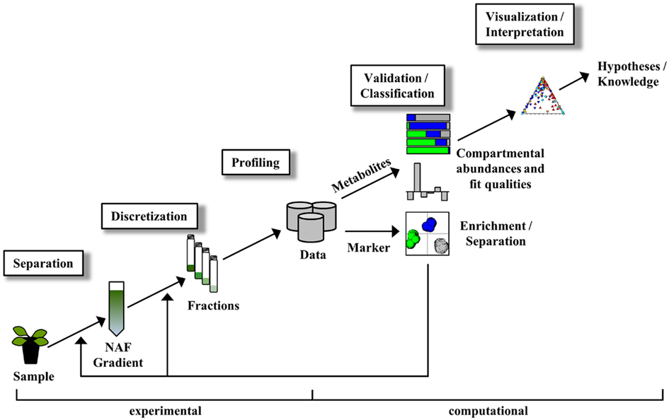
Figure 1. Simplified scheme of non-aqueous fractionation procedure and associated data analysis steps. For details see manuscript text.
The experimental part encompasses the separation, discretization, and profiling of sample material (Figure 1). After sample processing, subcellular compartments are enriched at discrete positions within a continuous density gradient. The gradient can then be separated into a number of fractions of ideally equal volume for the subsequent determination of cellular constituents. The collected gradient fractions are analyzed with respect to both compartment-specific markers (to unambiguously designate a compartment) and cellular constituents (to estimate their compartmental abundances) either using targeted assays or high-throughput analytical technologies (Gerhardt and Heldt, 1984; Fettke et al., 2005; Benkeblia et al., 2007; Krueger et al., 2009, 2011).
The computational part comprises the validation, classification, visualization, and interpretation of the obtained data (Figure 1). As each step consists of various tasks achievable by using a multitude of computational approaches, we here only provide a short overview for comprehension.
Validation
While the fidelity of the obtained measurements first requires an evaluation, regardless the specific methodology employed, here validation focuses on the evaluation of the computed compartmental enrichments and separation. First, defined compartments must be delineated through the use of compartment-specific markers, which ideally represent compartments under investigation in an unambiguous manner. The enrichment of these markers is commonly depicted as bar plots (Riens et al., 1991; Winter et al., 1993; Farre et al., 2001) and, but less frequently, statistically supported by pairwise comparisons (e.g., Student’s t-test) of the fraction abundances of markers (Krueger et al., 2009, 2011). However, while this shows the compartmental enrichment, it does not easily provide a parameter for the topological separation of all considered compartments. Normalized distances (Eqs 2 and 4) estimated on fraction abundances can be used to measure the separation between compartments designated using a single or multiple markers (Krueger et al., 2011). The subsequent use of clustering and associated cluster validation techniques (Halkidi et al., 2001), such as gap statistic (Tibshirani et al., 2001), or resampling approaches (Suzuki and Shimodaira, 2006), are powerful tools to statistically validate the cohesions within and separation between compartments, especially if multiples markers representing the same compartment are assayed (Krueger et al., 2011).
Classification
The main goal of this step is to estimate the compartmental abundance by computing the amount of cellular constituents in each of the previously defined compartments. While this can be achieved using simple linear regression for an individual compartment (Gerhardt and Heldt, 1984; Benkeblia et al., 2007), other linear least squares algorithms are more flexible for this purpose as estimates for all considered compartments can be computed simultaneously which also facilitates the assessment of the overall fit quality. These include the frequently used best fit algorithm (BFA, Riens et al., 1991), as well the non-negative least squares algorithm (NNLS, Lawson and Hanson, 1995). Both BFA and NNLS solve a system of linear equations defined by the marker-resolved compartments to determine the compartmental abundance by minimizing the discrepancy between the measured and fitted fraction abundances. Moreover, the iteratively (BFA), or by using the active-set method (NNLS), estimated compartmental abundances are constrained and thus restricted to yield always positive (and biological meaningful) estimates. However, the summed amount over all considered compartments does not need to equal 100% when using NNLS (Krueger et al., 2011). While estimates of compartmental abundances are computationally obtained, their qualities still need to be evaluated using the remaining associated discrepancy, commonly expressed as Euclidean distance or a derivate of it (Krueger et al., 2011).
Visualization and interpretation
A visual representation of the derived compartmentalization can be displayed through the combination of textual and graphical formats to aid in data interpretation. The choice of the visualization format depends on the questions addressed, the computational approach chosen, and the scientist’s preferences. Typically the estimated compartmental distributions are provided in tabular format while the underlying fraction abundances are depicted as heat maps or are converted into cluster trees (Farre et al., 2001; Benkeblia et al., 2007; Krueger et al., 2009). A topological format may also be used to facilitate the inclusion of previous results or prior knowledge (Krueger et al., 2011). This can greatly aid in data interpretation, as the integration of enzyme localization or pathway properties can lead to new knowledge and facilitate hypotheses generation.
Non-Aqueous Fractionation – A Simulation Model
Due to limited availability of experimental data, a simulation model was developed in order to study the influence of parameters on the compartmental separation and the estimation of compartmental abundances from NAF gradient data. To approximate the distribution of cellular constituents, such as compartment-specific markers or metabolites, we used random sampling from a truncated normal distribution, defined by the mean and SD within an interval ranging from 0 to 30 units. This choice was primarily motivated by four reasons: First, we used the abovementioned interval as a NAF gradient can comprise up to 30 mL (cf. Krueger et al., 2011) and therefore numerical parameters can be compared and interpreted in the context of existing experimental gradients. Secondly, by using the mean, simulated distributions can be easily placed at any position in the virtual gradient. Thirdly, by increasing the SD we can transform a cellular constituent from being highly enriched to being approximately equally distributed throughout the gradient. Finally, the effects produced through modifying the mean and SD are simple to understand as they are common parameters used to describe experimental results.
A model to illustrate the influence of distribution parameters on a virtual NAF gradient with four resolved compartments is shown as Figure 2, while a model for five compartments can be found as Figure A1 in Appendix. In experimental data, the two terminal distributions would correspond to compartmental distributions observed for plastids and the vacuole in plant studies (Krueger et al., 2011), while the non-enriched compartment with approximately equal fraction abundances can be considered as “cytosol” (Figure 2A, Figure A1A in Appendix). Whereas the exact characteristics of the distributions are shown as line plots (Figure 2A, Figure A1A in Appendix), experimentally only the discretized distributions can be assessed, i.e., the abundance of a cellular constituent throughout sampled gradient fractions (Figure 2B, Figure A1B in Appendix). When the SD is increased, the fraction abundances for the enriched compartments become closer to the non-enriched compartment (Figure 2B, Figure A1B in Appendix). Contrarily, increasing the marker spread by positioning markers representing the same compartment more distant from each other, the variation around the mean is increased (Figure 2B, Figure A1B in Appendix).
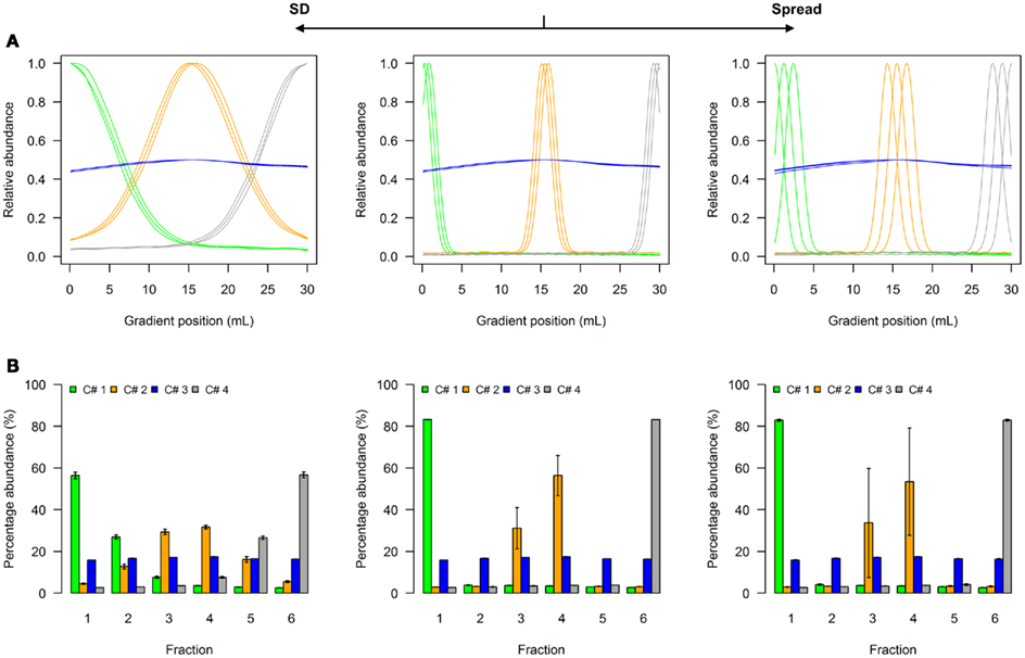
Figure 2. Simplified scheme of the four-compartmental simulation model. (A) The continuous distributions are depicted by line plots for each of the 4 compartments represented by 3 individual marker distributions. To aid visualization the distributions are scaled to half-maximum (blue-colored compartment) or maximum (all other) observed values. (B) The bar plots show the mean–averaged fraction abundances including SD among compartment-specific markers for each compartment after the continuous distributions were discretized into 6 equally spaced fractions. The left–side graph illustrates the effect of increasing the SD (SD = 5, ms = 0.4), while the right-side graph shows the effect of increasing the marker spread ms (SD = 1, ms = 1.2) compared to a standard (middle graph with SD = 1, ms = 0.4).
To show the behavior of the BCS and the WCC in dependence of changing SD and marker spreads, simulations were conducted individually for virtual NAF gradients containing either 3, 4, or 5 compartments each represented by 2, 3, or 5 markers, respectively. All combinations were tested using 2–30 fractions with 60 different SDs and 12 marker spread values each randomly repeated 99 times (see Materials and Methods). Both the BCS and the WCC were estimated on normalized Manhattan distances and visualized (Figure 3). Figure 3A clearly shows that with increasing SDs the BCS declines almost exponentially as the fraction abundances of compartmental markers become more similar to each other (Figure 2B, Figure A1B in Appendix), while the marker spread has minimal to no effect on the BCS. Contrarily, the WCC (Figure 3B) is influenced primarily by the marker spread, however, it is also affected by the compartmental separation modulated using the SD. Essentially the largest cohesion (i.e., the smallest distance) is observed at a high marker spread when the markers representing individual compartments are sharply focused at a specific gradient position (right bottom corner of Figure 3B).
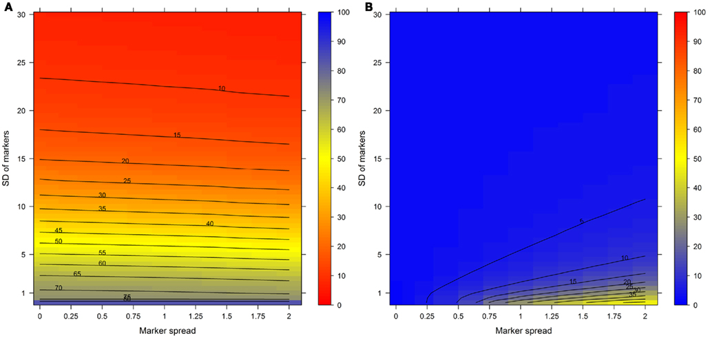
Figure 3. (A) The between-compartment separation and (B) the within-compartment cohesion in dependence of the SD and marker spread. Both indices were estimated as mean–average of normalized, percentage-scaled Manhattan distances either (A) between or (B) within-compartmental clusters and are depicted as level plots color-coded according to the right-sided color bars. To aid interpretation, lines have been drawn at each 5% level. The closer the between-compartment separation is to 100% the better the separation while the closer the within-compartment cohesion is to 0 the tighter the compartmental clusters.
How Many Fractions are Necessary to Produce a Good Separation?
The answer is a trade-off between technical difficulties in generating highly reproducible gradients, the sampling of the same amount of liquid from gradients (fractionation), how much material is required for the down-stream analytical technologies to be used, and the analytical workload associated with taking more fractions. While this is truly a question of experimental constraints, from the computational point of view limits can be deduced.
For this we used the simulated data generated as described above. To quantitatively evaluate the clustering results we used the mean–average of the average Silhouette information and the Pearson’s matrix correlation as the NAF validity index. Figure 4 illustrates this index with respect to the BCS (modulated by the SD of the marker) and the WCC (modulated by the marker spread) in dependence of the number of fractions collected. The figure was generated irrespective of the number of compartments (3–5) and markers (2, 3, or 5) per compartment considered by taking the mean value of the NAF validity index for different values of fractions and markers. For more detailed results see Figures A2–A4 in Appendix depicting the individual results from simulations using 3, 4, or 5 compartments each represented by 3 independent compartmental markers.
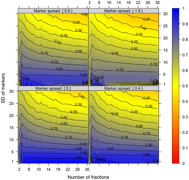
Figure 4. The cluster validity in dependence of the number of collected fractions, the SD of markers, and the marker spread. While the SD modulates the between-compartmental separation, the marker spread modulates the within-compartmental cohesion (cf. Figure 3). The cluster validity index, estimated as mean–average of the Silhouette information and the Pearson’s matrix correlation, is depicted independent of compartments (3–5) as well as markers (2, 3, or 5) per compartment considered. The closer the value is to 1 the better the observed cluster validity, color-coded as depicted in the right-side bar. To aid visualization negative cluster validity values were set to 0 and contour lines were drawn for each 0.05 unit. More detailed graphs can be found as Figures A2–A4 in Appendix.
While these figures first appear to be very complex, essentially the closer the values are to 1 (the bluer the color) the better the NAF validity index. Accordingly, we can conclude that the minimum number of fractions (nF) necessary to be collected should equal the number of compartments (nC) to be resolved, although similar cluster validities are also observed at nC −1 due to the inclusion of a non-enriched compartment (cf. Figure 2). The collection of a large number of small-volume fractions can result in the splitting of compartmental markers representing the same compartment, especially if markers are sharply focused (SD ≈ 1) and under increasing marker spreads. However, this can also happen when taking only a few fractions (see Figure 4, darker blue areas at SD ≈ 1 from left to right) but is more clearly evident when the number of fractions is increased. Finally, an increase in the number of fractions does not increase the cluster validity overall, i.e., there is no increase in the compartmental separation and thus the computationally estimated resolution of the gradient remains unchanged.
While this analysis only considers the compartmental separation, from the mathematical point of view there are constraints to the minimum number of fractions which should be taken. The least squares algorithms are usually applied to over-determined system of linear equations to yield an approximated solution, as otherwise an exact solution exists (Strang, 2009). In terms of the experimental system this means that there should be at least one more fraction used than the number of compartments which are to be determined, regardless if they are enriched or not. However, as it is desirable to apply additional constraints to the solution space (e.g., by restricting each variable to be positive and/or that all sum to 100%) even in cases where the number of fractions taken equals the number of compartments considered, a least squares approach, as opposed to an analytic solution, has to be employed as is the case for BFA or NNLS.
Therefore and in conclusion, the minimum number of fractions taken should ideally exceed the number of compartments. While the upper limit seems not to be definable, collecting a large number of fractions may led to compartment splitting which could be overcome by later combining and averaging the data from fractions known to be split. Nonetheless, it is rather important to determine the robustness of separation and compartmental boundaries in order to determine the experimentally optimal number of fractions and volumes to be collected. In some cases it may also be useful to take fractions of different volumes if the system under investigation is well defined or preliminary data with respect to compartmental boundaries is available.
Does the Fraction Number Influence the Compartmental Abundances?
To further address the influence of the number of fractions on the distribution of compartmental abundances we used the previously generated experimental data (Krueger et al., 2011). To modify the number of fractions we averaged either the terminal neighboring fractions 1 + 2 (plastidic enriched) and 5 + 6 (vacuolar enriched), resulting in 4 fractions (Figure 5A), or all neighboring fractions (1 + 2, 3 + 4, and 5 + 6) resulting in 3 fractions (Figure A5A in Appendix).
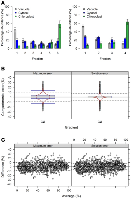
Figure 5. Influence of the number of collected fraction on estimated compartmental abundances based on experimental data. (A) Bar plots depicting the mean–averages and SDs of the three compartment-specific markers for each of the three resolved compartments on the basis of 6 and 4 collected fractions. Neighboring terminal fractions, i.e., 1 + 2 and 5 + 6, were averaged to obtain results for 4 fractions. (B) Combined box- and violin plots (red lines) as well as (C) mean-difference plots showing the difference of the maximum and solution error based on compartmental abundances estimated using BFA for gradients comprising 6 and 4 fractions. For both, positive values indicate larger compartmental abundances for 6 fractions while negative values depict larger abundances for 4 fractions. The 5th and 95th percentiles are drawn as black dashed lines. The figures show the average of three independent gradients.
First, we evaluated the compartmental cluster solutions which revealed silhouette information of 0.63 ± 0.03, 0.68 ± 0.02, and 0.76 ± 0.01 and Pearson’s matrix correlations of 0.74 ± 0.01, 0.75 ± 0.01, and 0.77 ± 0.02 for 6, 4, and 3 fractions, respectively (all as mean ± SD). Although an increase in both cluster validity indices were observed, indicating a better cohesion of and separation between compartments, the compartmental abundances of the individual markers were unchanged by reducing the fractions with, on average, 92.4 ± 8.9, 93.4 ± 7.5, and 93.3 ± 8.4% for 6, 4, and 3 fractions, respectively (all as mean ± SD) of the expected 100%. Comparing the differences of compartmental abundances for all metabolites based on 6 versus 4 or 3 fractions revealed rather narrow difference distributions (Figure 5B, Figure A5B in Appendix) independent of the observed mean values (Figure 5C, Figure A5C in Appendix) for both the maximum and the solution error. Using 4 fractions, 90% of all differences are within −8.7 to 10% and −6.7 to 7% for the maximum and solution error, respectively (Figures 5B,C). Similarly, using 3 fractions, 90% of all differences are in range from −8 to 13% and −8 to 9% for both the maximum and the solution error (Figures A5B,C in Appendix). While only minor effects were observed with respect to the compartmental abundances, reducing the fractions increased the number of sufficiently explained BFA estimates from 81.5% (TPD ≤ 10%), to 94.4% (TPD ≤ 9.4%) and 93.1% (TPD ≤ 7.4%) for 4 and 3 fractions, respectively. However, while this result is an enhancement, the reduced distribution space produced by shrinking the number of fractions effectively removes potential biologically meaningful intermediate distributions which are not delineated by the compartment-specific markers. Therefore, potential, yet-unresolved compartments can be overlooked. For instance, using 6 fractions, citrate synthase, a marker considered specific for the mitochondrial compartment (Stitt et al., 1982), has an insufficiently explained compartmental distribution (cf. Krueger et al., 2011). However, using 4 or 3 fractions, it is sufficiently explained with a 40% plastidic and 60% cytosolic distribution. Note that while the main isoform of citrate synthase is located in mitochondria, other isoforms are known to be present within the peroxisomes. These have been implicated in fatty acid respiration during seedling development and senescence (Pracharoenwattana et al., 2005; Kunz et al., 2009).
In conclusion, reducing the number of fractions only marginally influences the compartmental separation and the estimation of compartmental abundances. However, it does reduce the potential of detecting unknown, potentially fully resolved compartments. Therefore, increasing the number of fractions might enhance the detection of yet unassigned subcellular distribution and potential designation of a yet-unresolved or unconsidered compartment, especially if un-supervised “marker-free” approaches are employed (cf. Krueger et al., 2011).
Does the Marker Choice Influence the Estimated Compartmental Abundances?
Compartment-specific markers are central to NAF analyses as they anchor and establish the compartmental boundaries, and are ultimately used to estimate the compartmental abundances of the measured cellular constituents. Therefore the selection of certain cellular components as markers may influence the down-stream analysis and validity of the resulting data. Theoretically, the use of an unspecific marker (a marker that is shared between compartments or simply not localized to that compartment) would lead to erroneous conclusions. For example, although mannosidase enzyme activity has been widely used as a vacuolar marker in previously NAF studies (Gerhardt and Heldt, 1984; Riens et al., 1991; Winter et al., 1993; Farre et al., 2001; Benkeblia et al., 2007), recent experimental data from Arabidopsis showed activity in the Golgi (Strasser et al., 2006). This result questions the validity of using this marker specifically in Arabidopsis.
The use of multiple markers designating the same compartment can balance for a potential non-specificity of markers or their measurement errors. To test the importance of this factor we used the experimental NAF data where each of the resolved compartments (cytosol, plastid, and vacuole) is represented by three compartment-specific markers. First, we estimated how strong the compartmental abundance would be influenced by using jackknife approaches where we deleted a single marker, or used a marker twice. Although there are influences with respect to the cluster validity and BCS, for both the majority of observed values lay in a range of ±4% (Figures A6A,B in Appendix). Furthermore, all combinations of removing a marker or considering a marker twice do not largely influence the estimated compartmental abundances, compared to using all markers (Figures A6C,D in Appendix). Essentially, using one marker twice (Figure A6D in Appendix) led to very similar compartmental abundance, as 90% of all estimates were in range of −2.7 to 3% for the maximum error and −2.3 to 2.3% for the solution error. A similar, but slightly larger bias was observed with the omission of a marker with −5 to 5.7% for the maximum error and −4 to 4.3% for the solution error. Interestingly, the deletion or addition of a cytosolic marker influenced the estimates more strongly as compared to vacuolar or plastid-specific markers (Figures A6C,D in Appendix). This is in agreement with previous analyses, as it has been noted that the cytosolic compartment will cluster separately into three sub-clusters (Krueger et al., 2011). To further illustrate the effects of marker combinations and thus marker choice on compartmental abundances, we computed the compartmental abundances for each non-redundant marker combination. In contrast to the jackknife approaches, the distributions of differences are more heterogeneous. Here, 90% of the values over all marker combinations are in a range of −16 to 21.7% for the maximum error and −13.7% to 15.3% for the solution error (Figure 6). This illustrates that there is a clear influence on compartmental abundance estimation depending on the marker selected to represent a compartment. Therefore, by using multiple markers which ideally comprise the entire compartmental distribution space, the bias toward individual combinations can be reduced either by averaging prior to the estimation of compartmental abundances, or by averaging the compartmental abundances estimated using all non-redundant combinations (cf. Krueger et al., 2011).
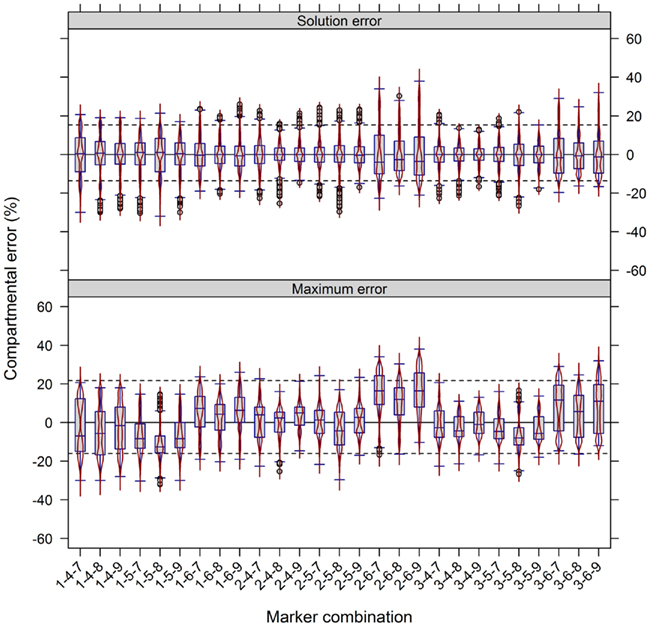
Figure 6. Influence of compartment-specific marker combinations on estimated compartmental abundances based on experimental data. Combined box- and violin plots (red lines) showing the difference of the maximum and solution error based on compartmental abundances estimated using BFA as mean–average difference over the three independent gradients. While positive values indicate larger compartmental abundances when all nine markers were used, negative values depict larger abundances for a certain 3-marker combination. The 5th and 95th percentiles among all combinations are drawn as black dashed lines. Marker 1–3, 4–6, and 7–9 represent the plastids, the cytosol, and the vacuole, respectively. Plastids: 1 – glyceraldehyde-3-phosphate dehydrogenase (GAPDH), 2 – starch, 3 – Digalactosyldiacylglycerols (DGDGs); Cytosol: 4 – Uridine diphosphate – glucose-pyrophosphorylase (UGPase), 5 – glyceroceramids (GlcCer), 6 – triacylglycerides (TAGs); Vacuole: 7 – nitrate, 8 – glucosinolates, and 9 – flavonoids.
How Good Must the Separation be to Get Reasonable Estimates of Compartmental Abundances?
In order to show the influence of the BCS and the metabolite error on compartmental abundance estimation, simulations were conducted individually for virtual NAF gradients containing either 3, 4, or 5 compartments each represented by two markers with 6, 9, or 12 considered fractions, respectively, and for all 60 SDs. The BCSs were estimated with normalized Manhattan distances (percentage scale) and binned in steps of 5% from 5 to 75. Differences in compartmental abundances were compared for each of the 300 gradient positions separately between the error-free and the error-containing distribution if the TPD did not exceed 15%. For all models and combinations of metabolite error and BCS bins, 200–1800 random estimates of compartmental abundances were considered.
Figure 7 illustrates the compartmental error with respect to the BCS and the cellular constituent error irrespective of the number of compartments (3–5) and fractions (6, 9, or 12) considered by taking the mean of the cellular constituent error for different values of the number of compartments and fractions. For more detailed results see Figures A7 and A8 in Appendix depicting the individual results of the compartmental errors for the compartments and fractions considered. As expected, the error in compartmental abundance estimation shows a clear dependence on both variables – the BCS and cellular constituent error (diagonal contours). Generally, the error of compartmental abundances increases rapidly with small increases of the cellular constituent error and small decreases of the BCS (Figures 7A,B). When considering the mean (Figure 7A) of all errors of compartmental abundances obtained for each binned value of BCS and cellular constituent error, both variables seem to contribute almost equally. However when considering the magnitude in the error of compartmental abundance, here derived by taking the 99th percentile (Figure 7B) of all computed values, a stronger influence of the cellular constituent error can be seen, illustrated as the much larger area of high errors of compartmental abundances, indicated by the dark red shading. This shows that the risk of obtaining high errors of compartmental abundances is more likely when the individual error of a cellular constituent is high, rather than with a low BCS. For experimentally obtained data, this would mean that the individual measurement accuracy of fraction abundances and the associated measurement error influence the compartmental abundance estimation stronger than the overall compartmental separation.
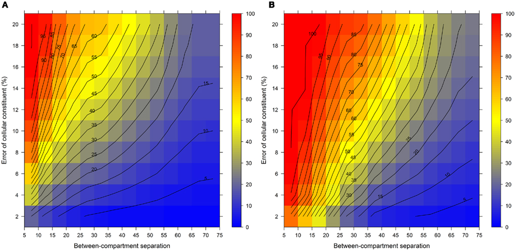
Figure 7. Calculation error of compartmental abundances in dependence of the between-compartment separation and the metabolite error based on simulated data. The estimated error, the discrepancies to the estimates of the error-free distributions, are depicted as (A) mean–average and (B) 99th percentile for each combination of between-compartment separation and metabolite error independent of the number of compartments (3–5) and fractions (6, 9, and 12) considered. The closer the value is to 0% the smaller the maximum error of the compartmental abundances, color-coded as depicted in the right-side bar. Contour lines have been drawn for each 5% error. More detailed graphs can be found as Figures A7 and A8 in Appendix.
To validate this, we performed a similar analysis on the experimental data (Figure 8). Similarly, the error in compartmental abundances increased almost exponentially with the increasing metabolite error, irrespective of either the maximum or the solution error. At the 10% metabolite error level the majority of differences in estimated compartmental abundances revealed a ∼10% compartmental error. When the metabolite error was increased further, the compartmental error rose rapidly to the point where the majority of absolute values reside in the range of up to 30%.
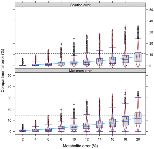
Figure 8. Calculation error of compartmental abundances in dependence of the metabolite error based on experimental data. Compartmental abundances are estimated using BFA and visualized as absolute mean–average difference over the three independent gradients. The 95th percentile among all metabolite error levels is drawn as black dashed lines. The light-blue solid line shows a fitted smooth curve to illustrate the increase of the estimated compartmental error with increasing metabolite error.
In conclusion, both simulated and experimental data revealed a larger effect of the measurement error of a cellular constituent on estimated compartmental abundances compared to the overall separation of compartments. To balance for these effects, the number of technical (ideally biological) replicates could be increased to obtain more robust compartmental estimates, thus increasing the confidence of the estimated subcellular metabolite distributions.
How Accurate Must a Least Squares Solution be to be Considered Statistically Valid?
The quality or the “goodness of fit” of any statistical model describes how well a set of observed data points fit to the estimated values the model returns. In our case this corresponds to how well the measured fraction abundances match the fitted ones determined by BFA or NNLS. Classically, the fit quality is quantified as the distance between the measured and estimated model data. Here, the residual sum of squares (RSS) or the Euclidean distance (the square-rooted RSS) is used where a small, closer to zero value indicates a “good fit.” However, since both measures are unscaled (unadjusted), it impedes interpretation of the fit quality. While TPD employs a normalized Manhattan distance to map distances on a percentage scale (Krueger et al., 2011), here we additionally suggest the use of a normalization of the Euclidean distance (Eq. 4), which is very closely related to the distance parameter a least squares approach tries to minimize.
Conceptually, one wants to use the discrepancy to decide whether a cellular constituent can be partitioned with confidence into the delineated subcellular compartments. The reason for investigating the fit quality by any of the mentioned measures is because a cellular constituent can display, compared to the fraction abundances of the marker, intermediate fraction abundances or a unique pattern that does not coincide with any considered marker/compartmental pattern. Both BFA and NNLS try to derive a predictive model assigning this cellular constituent into one of the defined subcellular compartments by using the observed marker distributions. Both algorithms will therefore result in a relatively high discrepancy and thus an incorrect classification of the cellular constituent with respect to its abundances in the considered compartments. However, in order to detect such cases, one needs to qualify or statistically quantify such a relatively high discrepancy.
While this could be achieved by arbitrarily defining a threshold to consider discrepancies as being acceptable, the threshold could also be adaptively inferred by employing a topological measure. For this purpose we use the degree of cohesion, defined by the spatial distance of the markers to their respective compartmental centers, either between independent gradients (Krueger et al., 2011) or within a gradient (applicable when multiple markers are assayed). We assume that the topological space a cellular constituent occupies cannot be larger than the one observed for the resolved compartments. Therefore, if the observed discrepancy for a cellular constituent exceeds the topological space of the compartments, the marker does not encompass its compartmentalization either due to potential transport processes or due to an unconsidered compartment. By assuming normality of the cohesion, one can express the divergence of an observed fit-discrepancy to this topological measure by standard (z-) scores, indicating how many SD a particular fit-discrepancy differs from the mean of the distances as defined by the compartmental cohesion. While negative values reflect discrepancies below the mean compartmental cohesion, positive values show discrepancies above the mean. Also, by employing a standard normal distribution function (e.g., pnorm in R), one can devise a right-tailed test to obtain p-values to further assess the statistical significance of the measured distributions.
BestFit – Further Developments and Current Implementation
As previously mentioned (Krueger et al., 2011), for fast computation on large data sets both least squares algorithms were implemented (BFA) or compiled (NNLS; Fortran 77 routine from R’s “nnls” package; Katharine and Van Stokkum, 2010) into the BestFit C-language command line tool (v1.1; Steinhauser et al., unpublished). In order to further enhance the calculation and evaluation of subcellular metabolite distributions from NAF data we have restructured and added further statistical analyses routines. In the current version (v1.2), BestFit supports the automatic calculation of compartmental cluster statistics, such as BCS, WCC, silhouette information, z-score estimation, and Pearson’s matrix correlation, based on both normalized Euclidean as well as Manhattan distances. Using the −A option (if multiple markers designating the same compartment are assayed) the user can control if the compartmental center or all marker combinations should be used to compute compartmental abundances for cellular constituents. Per default (−M option), markers are included in this analysis, i.e., treated as cellular constituents. To evaluate the fit quality the user can specify the cutoff (−T option; default to “max”) adaptively estimated either using the distance to the compartmental center (default) or the WCC using the −W option.
We observed when using NNLS that the sum of compartmental abundances for a solution equals the sum of fitted fraction abundances, even though the compartmental abundances do not need to sum to 100%. Interestingly, both the sums of fitted fractions and the compartmental abundances are perfectly correlated with a coefficient of determination of R2 = 1 (data not shown). Rescaling of the NNLS fitted fraction abundances followed by re-calculation using NNLS bound the sum of estimated compartmental abundances to 100% (termed NNLSs). To compare the difference in compartmental abundances estimated using BFA and NNLS or NNLSs we computed the LSS using a three- or four-compartmental model (the mitochondrial compartment was for this purpose considered as being unambiguously resolved) on the experimental data (Figure 9 and Figure A9 in Appendix). When 3 compartments are considered, 90% of all differences (TPD ≤ 10%) are within −1 to 0.9% and −0.8 to 0.8% for NNLSs while reveling for NNLS a larger spread, namely from −4.7 to 2.6% and −1.4 to 2%, for the maximum and solution error, respectively, compared to BFA (Figure 9). Similarly, using 4 compartments, 90% of all differences fall in the range from −0.8 to 1.6% and −0.7 to 0.7% for both the maximum and the solution error (Figure A9 in Appendix). As BFA uses a 1% interval to iteratively compute compartmental abundances, a large fraction of the observed differences fall within this range of ± 1% or can be the result of error propagation. Compared to BFA, which is limited to 5 compartments due to run-time constrains, NNLS is applicable to more than 5 compartments and is guaranteed to find the optimal solution that satisfies the conditions (non-negative solution). Also, using NNLSs the compartmental estimates can be scaled. This can be advantageous for some visualization formats (see below). Although there might be more sophisticated algorithms for constrained-based LSS to obtain non-negative values that sum up to 100%, we find it useful to implement NNLSs, an iterative NNLS, where the user can decide to choose this using −I option (default is set to 1 iteration, i.e., NNLS).
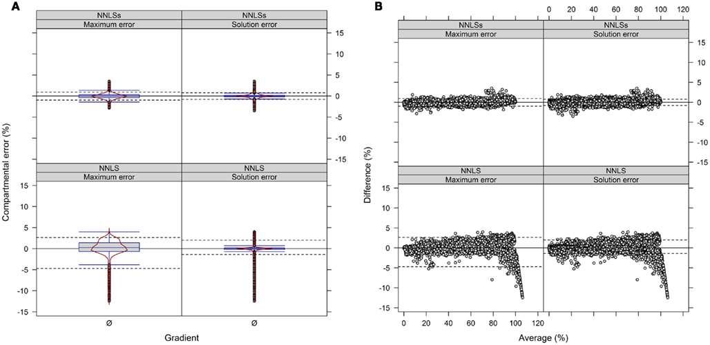
Figure 9. Diagnostic plots showing the differences in estimated compartmental abundances using (A,B) a three-compartmental estimation strategy based on experimental data. (A) The distributions of observed differences in compartmental abundances are shown as box- and violin plots (red lines). (B) The mean-difference plots depict the differences in dependence of the averages of compartmental abundances. For all graphs the difference in compartmental abundances between BFA and NNLS or iterative (seed-based) NNLS (NNLSs) are visualized based on the mean–average of compartmental abundances for the three independent gradients. The 5th and 95th percentiles are drawn as black dashed lines. Only values are shown if they are considered as sufficiently explained, i.e., TPD ≤ 10% based on the BFA solutions.
BestFit (v1.2) is available from CSB.DB website (Steinhauser et al., 2004) at http://csbdb.mpimp-golm.mpg.de/bestfit.html.
Visualization-Aided Interpretation of Data
While metabolic data has traditionally been visualized as cluster trees and their associated heat maps, we have attempted to focus on alternative types of visualization which can be easily overlaid or integrated with additional knowledge in order to achieve a more holistic overview of the data produced from NAF.
The use of PCo space, based on normalized Euclidean distances, is an excellent method to show the localization of the markers and associated metabolite classes or markers and compartment assignments through a visually appealing and easily interpretable figure (Figure 10). Here, the spatial spread of the markers clearly illustrates the heterogeneity of the considered classes across the entire space for metabolites from primary metabolism (Figure 10A), or the enrichment of the metabolite classes from secondary metabolism associated with specific compartments, such as the galactolipids in the chloroplast, the flavonoids or glucosinolates in the vacuole, or the triacylglycerides in the cytosol (Figure 10B). Using PCo space, the specificity for the metabolites assigned into a certain compartment or even between the compartments (for details on assignments see Krueger et al., 2011) can also be easily visualized (Figures 10C,D). Theoretically there is no limit to the number of compartments which may thus be shown. As this method greatly reduces the complexity of the data, the aid in biological interpretations is greatly increased.
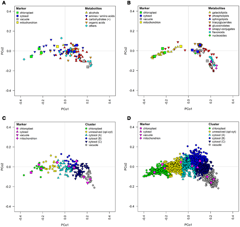
Figure 10. Topological maps of (A,C) primary metabolites as well as (B,D) secondary metabolites and lipids based on experimental data in proximity to resolved compartments. All graphs depict classification results visualized in principal coordinates (PCo) space on the basis of averaged normalized Euclidean distances among metabolites for the three independent gradients. (A,B) Chemical superclass assignments were overlaid on structurally identified metabolites and (C,D) k-medoids cluster assignments (cf. Krueger et al., 2011) were overlaid on all metabolites.
However, the data simplification for visualization using PCo space does not show the absolute compartmental enrichment or to what extent metabolites or classes of metabolites are shared between the analyzed compartments. Therefore the use of triangle plots is another useful way to present NAF derived data (Figure 11). They present the percent distribution of a certain metabolite, or group of metabolites shared between the different compartments, in an easily interpretable figure. In essence, this is the graphical equivalent of a tabulation of the data, as the estimated fraction amounts can be directly determined from the figure.
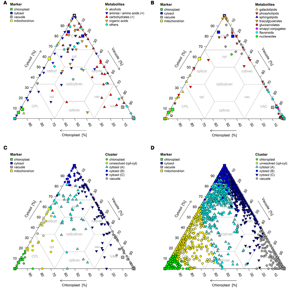
Figure 11. Triangle plots of (A,C) primary metabolites as well as (B,D) secondary metabolites and lipids based on estimated compartmental abundances for the three resolved compartments – plastids, the cytosol, and the vacuole. (A,B) Chemical superclass assignments were overlaid on structurally identified metabolites and (C,D) k-medoids cluster assignments (cf. Krueger et al., 2011) were overlaid on all metabolites.
For example, it is more obvious in a triangle plot that amines are closer associated to the chloroplast and cytosol than to the vacuole, that carbohydrates are more closely associated with the cytosol and vacuole, and that organic acids are more associated to the cytosol (Figure 11A). Just by eye, additional important information can be extracted. For example, only very few metabolites are located in the clp|cyt|vac space within the triangle plot, indicating that only few metabolites are equally shared between all three compartments (Figures 11A–D) and only a minor amount of metabolites show a distinct enrichment within the vacuole and the chloroplast, without being present in the cytosol. This is even more pronounced when depicted for all metabolites (Figure 11D). This is most likely due to the cytosol being the transit route between the other two compartments. One caveat for use of the triangle plot as a visualization tool is that the sum of the compartmental abundances must total 100%. Furthermore, it is only feasible for a three-compartmental separation.
Caveats and Benefits of Non-Aqueous Fractionation
Although several different approaches exist to study metabolite composition on the subcellular level, none can be referred to as “the method of choice” as every method has specific advantages and disadvantages. The best method to use depends on the experimental question.
First, the caveats: NAF is a generally labor intensive process and requires technical precision to produce consistent gradients. Secondly, analysis of the data from NAF gradients is critically dependent on the use of compartment-specific markers. The more markers used to define the compartmental space, and the more specific the markers are for a compartment, regardless of their biochemical nature, the better the resulting designation of the compartments. Until suitable markers are determined for the mitochondria or other unconsidered compartments, such as the peroxisome, or organelle sub-compartments, these structures must be considered unresolved. Finally, while the absolute purity of the isolated compartments in NAF gradients is not as tight as seen with protoplast fractionation or the perfusion technique, using statistical tests (as we have shown in this manuscript), high confidence data can clearly be produced from NAF gradients.
As for the benefits, the main one is that metabolism is effectively stopped immediately after harvesting. This prevents metabolite conversion or translocation, unlike protoplast fractionation (Robinson and Walker, 1979; Wirtz et al., 1980; Lilley et al., 1982; Stitt et al., 1989) and intracellular perfusion techniques (Takeshige and Tazawa, 1989).
Non-aqueous fractionation also produces an enrichment of the compartmental constituents, allowing for the potential detection of low-abundant compounds, such as hormones. As well, the relatively large amount of material used permits multiple down-stream analysis techniques to be applied, based on the number and volume of fractions taken. While we have routinely used GC/and LC/MS – based metabolomic approaches, this can easily be expanded toward the measurements of enzyme activities (Gibon et al., 2004; Steinhauser et al., 2010), proteomic-based technologies (Giavalisco et al., 2006), or to NMR (Weise et al., 2004). In the current age of systems biology the combination of comprehensive Omics technologies with classical NAF and modern computational biology approaches can dramatically increases the knowledge about the spatial and also temporal changes of metabolism on the subcellular level.
As NAF has been generally applied to whole organs or tissues, there has also been a concern of the contribution of the different cell types to the detected metabolite pools. As the Arabidopsis leaf is composed mainly of mesophyll cells, it can be assumed that these cells are the major contributor to the observed metabolite pool sizes. However, as shown previously, with a comprehensive enough or even specific analysis metabolites known to be spatially separated in different cell types can be localized to their experimentally proven compartments (Krueger et al., 2011).
Interestingly, because NAF separates not only intact organelles but also fragments of organelles, it might be also possible that identification of sub-organelle compartments may be achievable, such as the thylakoids from the stroma in chloroplasts, or dissecting the sub-compartments present in the plant vacuole (Paris et al., 1996), however this would require specific markers to delineate these compartments. For example, using NAF Riewe et al. (2008) could demonstrate that the apoplast of potato tuber is similarly, but not identically distributed as the vacuole in potato tubers. For Arabidopsis leaves, unassigned subcellular compartments could thus far only be identified by metabolite distributions that could not be explained by the three compartment-specific markers, strongly indicating the presence of additional subcellular compartments (Krueger et al., 2011).
Conflict of Interest Statement
The authors declare that the research was conducted in the absence of any commercial or financial relationships that could be construed as a potential conflict of interest.
Acknowledgments
This work was supported by the Max Planck Society and the University of Cologne. We thank the R Foundation for Statistical Computing and the R community for the continued development of the free software environment for statistical computing and graphics R. We would like to thank Dr. Björn Usadel for critical reading of this manuscript.
References
Albinsky, D., Kusano, M., Higuchi, M., Hayashi, N., Kobayashi, M., Fukushima, A., Mori, M., Ichikawa, T., Matsui, K., Kuroda, H., Horii, Y., Tsumoto, Y., Sakakibara, H., Hirochika, H., Matsui, M., and Saito, K. (2010). Metabolomic screening applied to rice FOX Arabidopsis lines leads to the identification of a gene-changing nitrogen metabolism. Mol. Plant 3, 125–142.
Bednarek, P., Pislewska-Bednarek, M., Svatos, A., Schneider, B., Doubsky, J., Mansurova, M., Humphry, M., Consonni, C., Panstruga, R., Sanchez-Vallet, A., Molina, A., and Schulze-Lefert, P. (2009). A glucosinolate metabolism pathway in living plant cells mediates broad-spectrum antifungal defense. Science 323, 101–106.
Benkeblia, N., Shinano, T., and Osaki, M. (2007). Metabolite profiling and assessment of metabolome compartmentation of soybean leaves using non-aqueous fractionation and GC-MS analysis. Metabolomics 3, 297–305.
Bowsher, C. G., and Tobin, A. K. (2001). Compartmentation of metabolism within mitochondria and plastids. J. Exp. Bot. 52, 513–527.
Brown, S. C., Kruppa, G., and Dasseux, J. L. (2005). Metabolomics applications of FT-ICR mass spectrometry. Mass Spectrom. Rev. 24, 223–231.
Büttner, M. (2007). The monosaccharide transporter(-like) gene family in Arabidopsis. FEBS Lett. 581, 2318–2324.
Carter, C., Pan, S., Zouhar, J., Avila, E. L., Girke, T., and Raikhel, N. V. (2004). The vegetative vacuole proteome of Arabidopsis thaliana reveals predicted and unexpected proteins. Plant Cell 16, 3285–3303.
Chen, L. Q., Hou, B. H., Lalonde, S., Takanaga, H., Hartung, M. L., Qu, X. Q., Guo, W. J., Kim, J. G., Underwood, W., Chaudhuri, B., Chermak, D., Antony, G., White, F. F., Somerville, S. C., Mudgett, M. B., and Frommer, W. B. (2010). Sugar transporters for intercellular exchange and nutrition of pathogens. Nature 468, 527–532.
Cox, T. F., and Cox, M. A. A. (1994). Multidimensional Scaling. Monographs on Statistics and Applied Probability. Boca Raton: Chapman and Hall/CRC.
Deuschle, K., Chaudhuri, B., Okumoto, S., Lager, I., Lalonde, S., and Frommer, W. B. (2006). Rapid metabolism of glucose detected with FRET glucose nanosensors in epidermal cells and intact roots of Arabidopsis RNA-silencing mutants. Plant Cell 18, 2314–2325.
Eisenhut, M., Ruth, W., Haimovich, M., Bauwe, H., Kaplan, A., and Hagemann, M. (2008). The photorespiratory glycolate metabolism is essential for cyanobacteria and might have been conveyed endosymbiontically to plants. Proc. Natl. Acad. Sci. U.S.A. 105, 17199–17204.
Emanuelsson, O., Nielsen, H., Brunak, S., and Von Heijne, G. (2000). Predicting subcellular localization of proteins based on their N-terminal amino acid sequence. J. Mol. Biol. 300, 1005–1016.
Farre, E. M., Fernie, A. R., and Willmitzer, L. (2008). Analysis of subcellular metabolite levels of potato tubers (Solanum tuberosum) displaying alterations in cellular or extracellular sucrose metabolism. Metabolomics 4, 161–170.
Farre, E. M., Tiessen, A., Roessner, U., Geigenberger, P., Trethewey, R. N., and Willmitzer, L. (2001). Analysis of the compartmentation of glycolytic intermediates, nucleotides, sugars, organic acids, amino acids, and sugar alcohols in potato tubers using a nonaqueous fractionation method. Plant Physiol. 127, 685–700.
Fehr, M., Frommer, W. B., and Lalonde, S. (2002). Visualization of maltose uptake in living yeast cells by fluorescent nanosensors. Proc. Natl. Acad. Sci. U.S.A. 99, 9846–9851.
Fernie, A. R. (2007). The future of metabolic phytochemistry: larger numbers of metabolites, higher resolution, greater understanding. Phytochemistry 68, 2861–2880.
Fernie, A. R., Trethewey, R. N., Krotzky, A. J., and Willmitzer, L. (2004). Metabolite profiling: from diagnostics to systems biology. Nat. Rev. Mol. Cell Biol. 5, 763–769.
Fettke, J., Chia, T., Eckermann, N., Smith, A., and Steup, M. (2006). A transglucosidase necessary for starch degradation and maltose metabolism in leaves at night acts on cytosolic heteroglycans (SHG). Plant J. 46, 668–684.
Fettke, J., Eckermann, N., Tiessen, A., Geigenberger, P., and Steup, M. (2005). Identification, subcellular localization and biochemical characterization of water-soluble heteroglycans (SHG) in leaves of Arabidopsis thaliana L.: distinct SHG reside in the cytosol and in the apoplast. Plant J. 43, 568–585.
Fettke, J., Hejazi, M., Smirnova, J., Hochel, E., Stage, M., and Steup, M. (2009). Eukaryotic starch degradation: integration of plastidial and cytosolic pathways. J. Exp. Bot. 60, 2907–2922.
Fiehn, O. (2001). Combining genomics, metabolome analysis, and biochemical modelling to understand metabolic networks. Comp. Funct. Genomics 2, 155–168.
Gerhardt, R., and Heldt, H. W. (1984). Measurement of subcellular metabolite levels in leaves by fractionation of freeze-stopped material in nonaqueous media. Plant Physiol. 75, 542–547.
Giavalisco, P., Kapitza, K., Kolasa, A., Buhtz, A., and Kehr, J. (2006). Towards the proteome of Brassica napus phloem sap. Proteomics 6, 896–909.
Gibon, Y., Blaesing, O. E., Hannemann, J., Carillo, P., Hohne, M., Hendriks, J. H., Palacios, N., Cross, J., Selbig, J., and Stitt, M. (2004). A Robot-based platform to measure multiple enzyme activities in Arabidopsis using a set of cycling assays: comparison of changes of enzyme activities and transcript levels during diurnal cycles and in prolonged darkness. Plant Cell 16, 3304–3325.
Gout, E., Aubert, S., Bligny, R., Rebeille, F., Nonomura, A. R., Benson, A. A., and Douce, R. (2000). Metabolism of methanol in plant cells. Carbon-13 nuclear magnetic resonance studies. Plant Physiol. 123, 287–296.
Gout, E., Bligny, R., Pascal, N., and Douce, R. (1993). 13C nuclear magnetic resonance studies of malate and citrate synthesis and compartmentation in higher plant cells. J. Biol. Chem. 268, 3986–3992.
Gutscher, M., Pauleau, A. L., Marty, L., Brach, T., Wabnitz, G. H., Samstag, Y., Meyer, A. J., and Dick, T. P. (2008). Real-time imaging of the intracellular glutathione redox potential. Nat. Methods 5, 553–559.
Halkidi, M., Batistakis, Y., and Vazirgiannis, M. (2001). On clustering validation techniques. J. Intell. Inf. Syst. 17, 107–145.
Hannah, M. A., Caldana, C., Steinhauser, D., Balbo, I., Fernie, A. R., and Willmitzer, L. (2010). Combined transcript and metabolite profiling of Arabidopsis grown under widely variant growth conditions facilitates the identification of novel metabolite-mediated regulation of gene expression. Plant Physiol. 152, 2120–2129.
Heazlewood, J. L., Verboom, R. E., Tonti-Filippini, J., Small, I., and Millar, A. H. (2007). SUBA: the Arabidopsis subcellular database. Nucleic Acids Res. 35, D213–218.
Heinrich, G., and Kuschki, B. (1978). Verluste radioaktiv markierter Substanzen aus Pisum-Wurzeln nach Verfütterung von D-Glucose-14C im Verlauf unterschiedlicher Präparationsmethoden für die Elektronenmikroskopie. Histochem. Cell Biol. 319–328.
Hennig, C. (2010). fpc: Flexible Procedures for Clustering. R package version 2.0–2. Available at: http://CRAN.R-project.org/package=fpc
Huege, J., Krall, L., Steinhauser, M. C., Giavalisco, P., Rippka, R., Tandeau De Marsac, N., and Steinhauser, D. (2011). Sample amount alternatives for data adjustment in comparative cyanobacterial metabolomics. Anal. Bioanal. Chem. 399, 3503–3517.
Jackson, C. (2010). msm: Multi-State Markov and Hidden Markov Models in Continuous Time. R package version 0.9.7. Available at: http://CRAN.R-project.org/package=msm
Jozefczuk, S., Klie, S., Catchpole, G., Szymanski, J., Cuadros-Inostroza, A., Steinhauser, D., Selbig, J., and Willmitzer, L. (2010). Metabolomic and transcriptomic stress response of Escherichia coli. Mol. Syst. Biol. 6, 364.
Junker, B. H., Wuttke, R., Nunes-Nesi, A., Steinhauser, D., Schauer, N., Bussis, D., Willmitzer, L., and Fernie, A. R. (2006). Enhancing vacuolar sucrose cleavage within the developing potato tuber has only minor effects on metabolism. Plant Cell Physiol. 47, 277–289.
Kaplan, F., Kopka, J., Haskell, D. W., Zhao, W., Schiller, K. C., Gatzke, N., Sung, D. Y., and Guy, C. L. (2004). Exploring the temperature-stress metabolome of Arabidopsis. Plant Physiol. 136, 4159–4168.
Kaplan, F., Kopka, J., Sung, D. Y., Zhao, W., Popp, M., Porat, R., and Guy, C. L. (2007). Transcript and metabolite profiling during cold acclimation of Arabidopsis reveals an intricate relationship of cold-regulated gene expression with modifications in metabolite content. Plant J. 50, 967–981.
Katharine, M. M., and Van Stokkum, I. H. M. (2010). nnls: The Lawson-Hanson Algorithm for Non-Negative Least Squares (NNLS). R package version 1.3. Available at: http://CRAN.R-project.org/package=nnls
Kopka, J., Fernie, A., Weckwerth, W., Gibon, Y., and Stitt, M. (2004). Metabolite profiling in plant biology: platforms and destinations. Genome Biol. 5, 109.
Krueger, S., Donath, A., Lopez-Martin, M. C., Hoefgen, R., Gotor, C., and Hesse, H. (2010). Impact of sulfur starvation on cysteine biosynthesis in T-DNA mutants deficient for compartment-specific serine-acetyltransferase. Amino Acids 39, 1029–1042.
Krueger, S., Giavalisco, P., Krall, L., Steinhauser, M. C., Bussis, D., Usadel, B., Flugge, U. I., Fernie, A. R., Willmitzer, L., and Steinhauser, D. (2011). A topological map of the compartmentalized Arabidopsis thaliana leaf metabolome. PLoS ONE 6, e17806. doi: 10.1371/journal.pone.0017806
Krueger, S., Niehl, A., Lopez Martin, M. C., Steinhauser, D., Donath, A., Hildebrandt, T., Romero, L. C., Hoefgen, R., Gotor, C., and Hesse, H. (2009). Analysis of cytosolic and plastidic serine acetyltransferase mutants and subcellular metabolite distributions suggests interplay of the cellular compartments for cysteine biosynthesis in Arabidopsis. Plant Cell Environ. 32, 349–367.
Kruger, N. J., and Von Schaewen, A. (2003). The oxidative pentose phosphate pathway: structure and organisation. Curr. Opin. Plant Biol. 6, 236–246.
Kunz, H. H., Scharnewski, M., Feussner, K., Feussner, I., Flugge, U. I., Fulda, M., and Gierth, M. (2009). The ABC transporter PXA1 and peroxisomal beta-oxidation are vital for metabolism in mature leaves of Arabidopsis during extended darkness. Plant Cell 21, 2733–2749.
Kusano, M., Tohge, T., Fukushima, A., Kobayashi, M., Hayashi, N., Otsuki, H., Kondou, Y., Goto, H., Kawashima, M., Matsuda, F., Niida, R., Matsui, M., Saito, K., and Fernie, A. R. (2011). Metabolomics reveals comprehensive reprogramming involving two independent metabolic responses of Arabidopsis to ultraviolet-B light. Plant J. 67, 354–369.
Lalonde, S., Ehrhardt, D. W., and Frommer, W. B. (2005). Shining light on signaling and metabolic networks by genetically encoded biosensors. Curr. Opin. Plant Biol. 8, 574–581.
Lawson, C. L., and Hanson, R. J. (1995). Solving Least Squares Problems. Classics in Applied Mathematics. Philadelphia: SIAM.
Libourel, I. G., Van Bodegom, P. M., Fricker, M. D., and Ratcliffe, R. G. (2006). Nitrite reduces cytoplasmic acidosis under anoxia. Plant Physiol. 142, 1710–1717.
Lilley, R. McC., Stitt, M., Mader, G., and Heldt, H. W. (1982). Rapid fractionation of wheat leaf protoplasts using membrane filtration: the determination of metabolite levels in the chloroplasts, cytosol, and mitochondria. Plant Physiol. 70, 965–970.
Martinoia, E., Maeshima, M., and Neuhaus, H. E. (2007). Vacuolar transporters and their essential role in plant metabolism. J. Exp. Bot. 58, 83–102.
Meyer, R. C., Steinfath, M., Lisec, J., Becher, M., Witucka-Wall, H., Torjek, O., Fiehn, O., Eckardt, A., Willmitzer, L., Selbig, J., and Altmann, T. (2007). The metabolic signature related to high plant growth rate in Arabidopsis thaliana. Proc. Natl. Acad. Sci. U.S.A. 104, 4759–4764.
Mugford, S. G., Yoshimoto, N., Reichelt, M., Wirtz, M., Hill, L., Mugford, S. T., Nakazato, Y., Noji, M., Takahashi, H., Kramell, R., Gigolashvili, T., Flugge, U. I., Wasternack, C., Gershenzon, J., Hell, R., Saito, K., and Kopriva, S. (2009). Disruption of adenosine-5’-phosphosulfate kinase in Arabidopsis reduces levels of sulfated secondary metabolites. Plant Cell 21, 910–927.
Pan, Z., and Raftery, D. (2007). Comparing and combining NMR spectroscopy and mass spectrometry in metabolomics. Anal. Bioanal. Chem. 387, 525–527.
Paris, N., Stanley, C. M., Jones, R. L., and Rogers, J. C. (1996). Plant cells contain two functionally distinct vacuolar compartments. Cell 85, 563–572.
Peters, T. Jr., and Ashley, C. A. (1967). An artefact in radioautography due to binding of free amino acids to tissues by fixatives. J. Cell Biol. 33, 53–60.
Pracharoenwattana, I., Cornah, J. E., and Smith, S. M. (2005). Arabidopsis peroxisomal citrate synthase is required for fatty acid respiration and seed germination. Plant Cell 17, 2037–2048.
R Development Core Team. (2010). R: A Language and Environment for Statistical Computing. R Foundation for Statistical Computing, Vienna. ISBN 3-900051-07-0. Available at: http://www.R-project.org
Rébeillé, F., Alban, C., Bourguignon, J., Ravanel, S., and Douce, R. (2007). The role of plant mitochondria in the biosynthesis of coenzymes. Photosyn. Res. 92, 149–162.
Riens, B., Lohaus, G., Heineke, D., and Heldt, H. W. (1991). Amino acid and sucrose content determined in the cytosolic, chloroplastic, and vacuolar compartments and in the phloem sap of spinach leaves. Plant Physiol. 97, 227–233.
Riewe, D., Grosman, L., Fernie, A. R., Wucke, C., and Geigenberger, P. (2008). The potato-specific apyrase is apoplastically localized and has influence on gene expression, growth, and development. Plant Physiol. 147, 1092–1109.
Robinson, S. P., and Walker, D. A. (1979). Rapid separation of the chloroplast and cytoplasmic fractions from intact leaf protoplasts. Arch. Biochem. Biophys. 196, 319–323.
Rousseeuw, P. J. (1987). Silhouettes: a graphical aid to the interpretation and validation of cluster analysis. J. Comput. Appl. Math. 20, 53–65.
Saito, K., and Matsuda, F. (2010). Metabolomics for functional genomics, systems biology, and biotechnology. Annu. Rev. Plant Biol. 61, 463–489.
Schauer, N., Semel, Y., Roessner, U., Gur, A., Balbo, I., Carrari, F., Pleban, T., Perez-Melis, A., Bruedigam, C., Kopka, J., Willmitzer, L., Zamir, D., and Fernie, A. R. (2006). Comprehensive metabolic profiling and phenotyping of interspecific introgression lines for tomato improvement. Nat. Biotechnol. 24, 447–454.
Schwacke, R., Schneider, A., Van Der Graaff, E., Fischer, K., Catoni, E., Desimone, M., Frommer, W. B., Flugge, U. I., and Kunze, R. (2003). ARAMEMNON, a novel database for Arabidopsis integral membrane proteins. Plant Physiol. 131, 16–26.
Sokal, R. R., and Rohlf, F. J. (1995). Biometry: The Principles and Practice of Statistics in Biological Research. New York: W. H. Freeman and Company.
Steinhauser, D., Usadel, B., Luedemann, A., Thimm, O., and Kopka, J. (2004). CSB.DB: a comprehensive systems-biology database. Bioinformatics 20, 3647–3651.
Steinhauser, M. C., Steinhauser, D., Koehl, K., Carrari, F., Gibon, Y., Fernie, A. R., and Stitt, M. (2010). Enzyme activity profiles during fruit development in tomato cultivars and Solanum pennellii. Plant Physiol. 153, 80–98.
Stitt, M., and Fernie, A. R. (2003). From measurements of metabolites to metabolomics: an “on the fly” perspective illustrated by recent studies of carbon-nitrogen interactions. Curr. Opin. Biotechnol. 14, 136–144.
Stitt, M., Lilley, R. M., Gerhardt, R., and Heldt, H. W. (1989). Determination of metabolite levels in specific cells and subcellular compartments of plant leaves. Meth. Enzymol. 174, 518–552.
Stitt, M., Lilley, R. M., and Heldt, H. W. (1982). Adenine nucleotide levels in the cytosol, chloroplasts, and mitochondria of wheat leaf protoplasts. Plant Physiol. 70, 971–977.
Stitt, M., Lunn, J., and Usadel, B. (2010a). Arabidopsis and primary photosynthetic metabolism – more than the icing on the cake. Plant J. 61, 1067–1091.
Stitt, M., Sulpice, R., and Keurentjes, J. (2010b). Metabolic networks: how to identify key components in the regulation of metabolism and growth. Plant Physiol. 152, 428–444.
Stitt, M., Wirtz, W., and Heldt, H. W. (1983). Regulation of sucrose synthesis by cytoplasmic fructosebisphosphatase and sucrose phosphate synthase during photosynthesis in varying light and carbon dioxide. Plant Physiol. 72, 767–774.
Strasser, R., Schoberer, J., Jin, C., Glossl, J., Mach, L., and Steinkellner, H. (2006). Molecular cloning and characterization of Arabidopsis thaliana Golgi alpha-mannosidase II, a key enzyme in the formation of complex N-glycans in plants. Plant J. 45, 789–803.
Sulpice, R., Pyl, E. T., Ishihara, H., Trenkamp, S., Steinfath, M., Witucka-Wall, H., Gibon, Y., Usadel, B., Poree, F., Piques, M. C., Von Korff, M., Steinhauser, M. C., Keurentjes, J. J., Guenther, M., Hoehne, M., Selbig, J., Fernie, A. R., Altmann, T., and Stitt, M. (2009). Starch as a major integrator in the regulation of plant growth. Proc. Natl. Acad. Sci. U.S.A. 106, 10348–10353.
Suzuki, R., and Shimodaira, H. (2006). Pvclust: an R package for assessing the uncertainty in hierarchical clustering. Bioinformatics 22, 1540–1542.
Sweetlove, L. J., Fell, D., and Fernie, A. R. (2008). Getting to grips with the plant metabolic network. Biochem. J. 409, 27–41.
Takeshige, K., and Tazawa, M. (1989). Determination of the inorganic pyrophosphate level and its subcellular localization in Chara corallina. J. Biol. Chem. 264, 3262–3266.
Taylor, N. L., Heazlewood, J. L., and Millar, A. H. (2011). The Arabidopsis thaliana 2-D gel mitochondrial proteome: refining the value of reference maps for assessing protein abundance, contaminants and post-translational modifications. Proteomics 11, 1720–1733.
Tibshirani, R., Walther, G., and Hastie, T. (2001). Estimating the number of clusters in a dataset via the gap statistic. J. R. Stat. Soc. Ser. B 63, 411–423.
Walker, R. P., Chen, Z. H., Johnson, K. E., Famiani, F., Tecsi, L., and Leegood, R. C. (2001). Using immunohistochemistry to study plant metabolism: the examples of its use in the localization of amino acids in plant tissues, and of phosphoenolpyruvate carboxykinase and its possible role in pH regulation. J. Exp. Bot. 52, 565–576.
Weber, A. P., and Fischer, K. (2007). Making the connections–the crucial role of metabolite transporters at the interface between chloroplast and cytosol. FEBS Lett. 581, 2215–2222.
Weise, S. E., Weber, A. P., and Sharkey, T. D. (2004). Maltose is the major form of carbon exported from the chloroplast at night. Planta 218, 474–482.
Winter, H., Robinson, D. G., and Heldt, H. W. (1993). Subcellular volumes and metabolite concentrations in barley leaves. Planta 191, 180–190.
Wirtz, W., Stitt, M., and Heldt, H. W. (1980). Enzymic determination of metabolites in the subcellular compartments of spinach protoplasts. Plant Physiol. 66, 187–193.
Yamada, K., Norikoshi, R., Suzuki, K., Imanishi, H., and Ichimura, K. (2009). Determination of subcellular concentrations of soluble carbohydrates in rose petals during opening by nonaqueous fractionation method combined with infiltration-centrifugation method. Planta 230, 1115–1127.
Zechmann, B., Stumpe, M., and Mauch, F. (2011). Immunocytochemical determination of the subcellular distribution of ascorbate in plants. Planta 233, 1–12.
Zeeman, S. C., Thorneycroft, D., Schupp, N., Chapple, A., Weck, M., Dunstan, H., Haldimann, P., Bechtold, N., Smith, A. M., and Smith, S. M. (2004). Plastidial alpha-glucan phosphorylase is not required for starch degradation in Arabidopsis leaves but has a role in the tolerance of abiotic stress. Plant Physiol. 135, 849–858.
Appendix
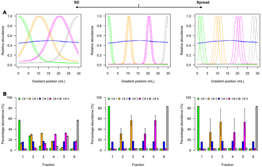
Figure A1. Simplified scheme of the five-compartmental simulation model. (A) The continuous distributions are depicted by line plots for each of the 5 compartments represented by 3 individual marker distributions. To aid visualization the distributions are scaled to half-maximum (blue-colored compartment) or maximum (all other) observed values. (B) The bar plots show the mean–averaged fraction abundances including SD among compartment-specific markers for each compartment after the continuous distributions were discretized into 6 equally spaced fractions. The left–side graph illustrates the effect of increasing the SD (SD = 5, ms = 0.4), while the right-side graph shows the effect of increasing the marker spread ms (SD = 1, ms = 1.2) compared to a standard (middle graph with SD = 1, ms = 0.4).
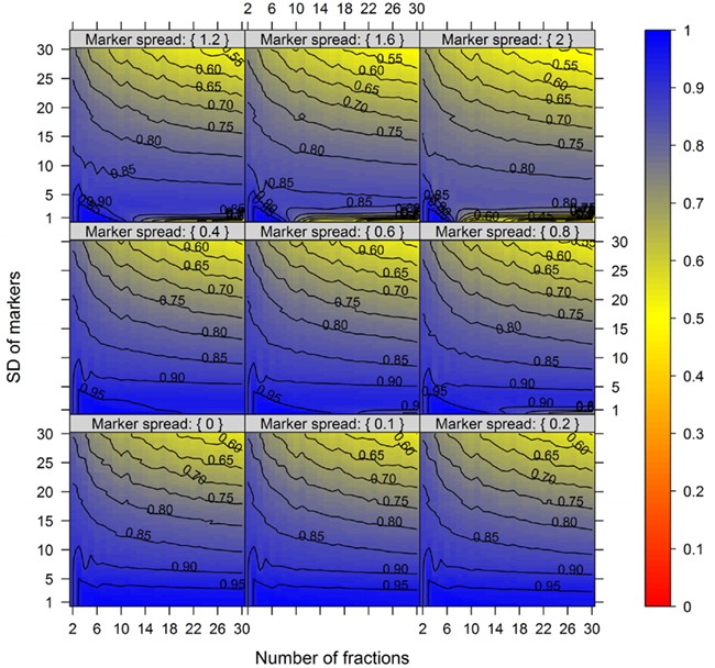
Figure A2. The cluster validity in dependence of the number of collected fractions, the SD of markers, and the marker spread for the three-compartmental model. While the SD modulates the between-compartmental separation, the marker spread modulates the within-compartmental cohesion (cf. Figure 3). The cluster validity index estimated as mean–average of the Silhouette information and the Pearson’s matrix correlation is depicted for 3 compartments each represented by 3 markers. The closer the value is to 1 the better the observed cluster validity, color-coded as depicted in the right-side bar. To aid visualization negative cluster validity values were set to 0 and contour lines were drawn for each 0.05 unit.
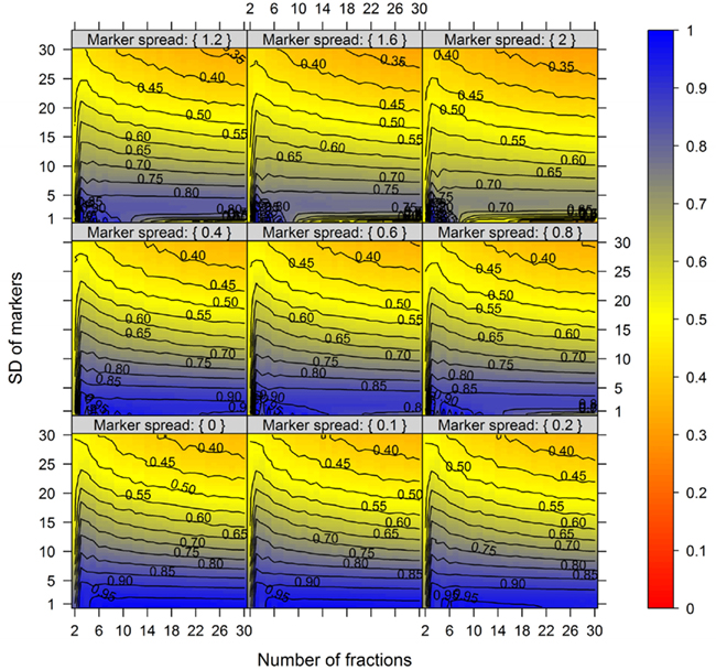
Figure A3. The cluster validity in dependence of the number of collected fractions, the SD of markers, and the marker spread for the four-compartmental model. The cluster validity index is depicted for 4 compartments each represented by 3 markers. For further details see Figure A2.
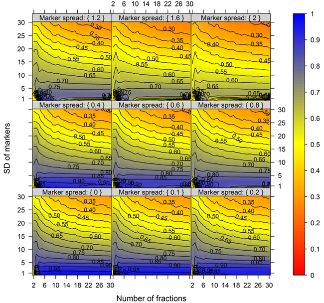
Figure A4. The cluster validity in dependence of the number of collected fractions, the SD of markers, and the marker spread for the five-compartmental model. The cluster validity index is depicted for 5 compartments each represented by 3 markers. For further details see Figure A2.
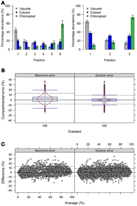
Figure A5. Influence of the number of collected fraction on estimated compartmental abundances based on experimental data. (A) Bar plots depicting the mean–averages and SDs of the three compartment-specific markers for each of the three resolved compartments on the basis of 6 and 3 collected fractions. Neighboring fractions, i.e., 1 + 2, 3 + 4, and 5 + 6, were averaged to obtain results for 3 fractions. (B) Combined box- and violin plots (red lines) as well as (C) mean-difference plots showing the difference of the maximum and solution error based on compartmental abundances estimated using BFA for gradients comprising 6 and 3 fractions. For both, positive values indicate larger compartmental abundances for 6 fractions while negative values depict larger abundances for 3 fractions. The 5th and 95th percentiles are drawn as black dashed lines. The figures show the average of three independent gradients.
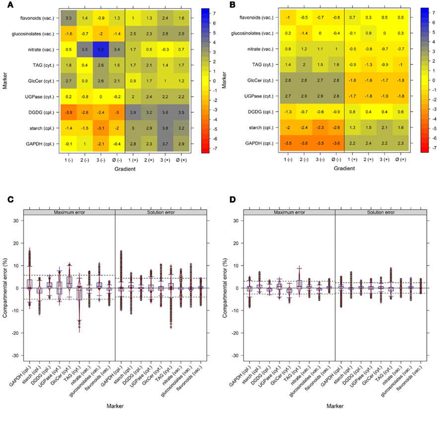
Figure A6. Influence of compartment-specific marker combinations on (A) cluster validity, (B) between-compartment separation, and (C,D) estimated compartmental abundances based on experimental data. (A) The cluster validity index, estimated as mean–average of the Silhouette information and the Pearson’s matrix correlation, and (B) the between-compartment separation are depicted as percentage difference from the cluster solution using all nine compartmental markers. The values are provided for all three independent gradients (1–3) and as mean–average (Ø) by deleting one marker (−; jackknife−) or taking one marker twice (+; jackknife+). (C,D) Combined box- and violin plots (red lines) showing the difference of the maximum and solution error based on compartmental abundances estimated using BFA when (C) deleting one marker or (D) considering one marker twice. All estimates are based on the difference observed after mean–average of the three independent gradients. Red squares in (C) depict the difference in the marker that was deleted. The 5th and 95th percentiles are drawn as black dashed lines. For both, positive values indicate larger compartmental abundances when all nine markers were used while negative values depict larger abundances when a marker was deleted or considered twice.
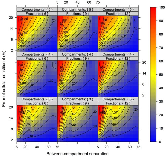
Figure A7. Mean–averaged calculation error of compartmental abundances in dependence of the between-compartment separation and the metabolite error based on simulated data. The estimated maximum error is depicted as mean–average for each combination of between-compartment separation and metabolite error in dependence of the number of compartments (3–5) and number of fraction (6, 9, and 12) considered. The closer the value is to 0% the smaller the error of the compartmental abundances (estimated using NNLS), color-coded as depicted in the right-side bar. Contour lines are drawn for each 10% error.
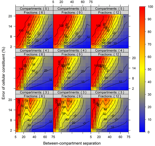
Figure A8. Percentile (99%) calculation error of compartmental abundances in dependence of the between-compartment separation and the metabolite error based on simulated data. The error is depicted as 99th percentile for each combination of between-compartment separation and metabolite error in dependence of the number of compartments (3–5) and number of fraction (6, 9, and 12) considered. For further details see Figure A7.
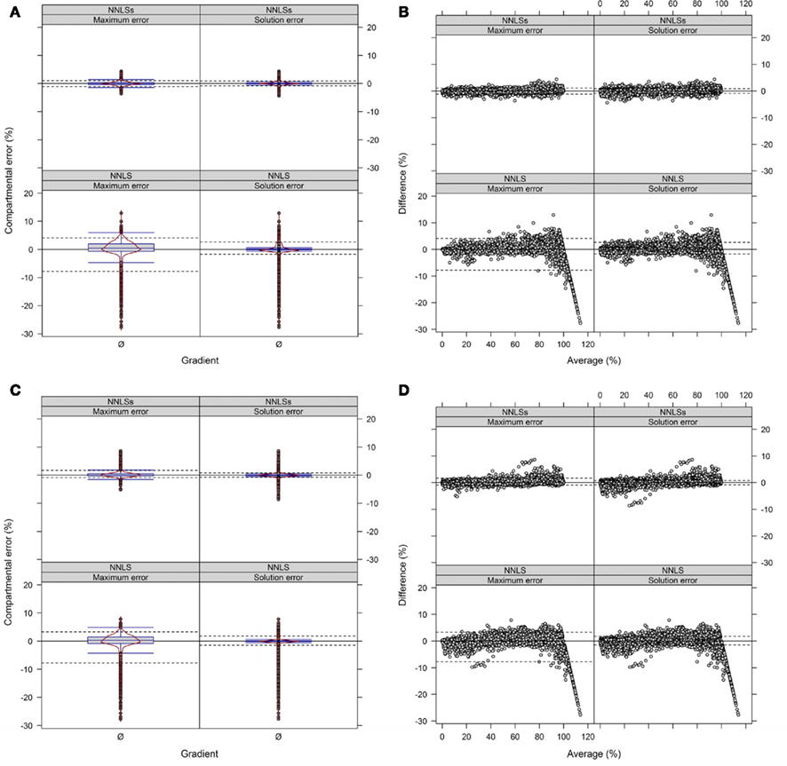
Figure A9. Diagnostic plots showing the differences in estimated compartmental abundances using (A,B) a three- and (C,D) a four-compartmental estimation strategy based on experimental data. (A,C) The distributions of observed differences in compartmental abundances are shown as box- and violin plots (red lines). (B,D) The mean-difference plots depict the differences in dependence of the averages of compartmental abundances. For all graphs the difference in compartmental abundances between BFA and NNLS or iterative (seed-based) (NNLSs) are visualized based on the mean–average of compartmental abundances for the three independent gradients. The 5th and 95th percentiles are drawn as black dashed lines. All values are shown, regardless if they are considered as sufficiently explained or not.
Keywords: subcellular metabolomics, analysis workflow, computational simulations, least squares algorithms, BestFit tool, visualization
Citation: Klie S, Krueger S, Krall L, Giavalisco P, Flügge U-I, Willmitzer L and Steinhauser D (2011) Analysis of the compartmentalized metabolome – a validation of the non-aqueous fractionation technique. Front. Plant Sci. 2:55. doi: 10.3389/fpls.2011.00055
Received: 01 May 2011;
Accepted: 05 September 2011;
Published online: 22 September 2011.
Edited by:
Alisdair Fernie, Max Planck Institute for Plant Physiology, GermanyReviewed by:
Alisdair Fernie, Max Planck Institute for Plant Physiology, GermanyLee Sweetlove, University of Oxford, UK
Copyright: © 2011 Klie, Krueger, Krall, Giavalisco, Flügge, Willmitzer and Steinhauser. This is an open-access article subject to a non-exclusive license between the authors and Frontiers Media SA, which permits use, distribution and reproduction in other forums, provided the original authors and source are credited and other Frontiers conditions are complied with.
*Correspondence: Dirk Steinhauser, Department of Molecular Physiology, Max Planck Institute of Molecular Plant Physiology, Am Mühlenberg 1, 14476 Potsdam-Golm, Germany. e-mail:c3RlaW5oYXVzZXJAbXBpbXAtZ29sbS5tcGcuZGU=
 Sebastian Klie1

