Relative roughness: an index for testing the suitability of the monofractal model

Fractal analyses have become very popular and have been applied on a wide variety of empirical time series. The application of these methods supposes that the monofractal framework can offer a suitable model for the analyzed series. However, this model takes into account a quite specific kind of fluctuations, and we consider that fractal analyses have been often applied to series that were completely outside of its relevance. The problem is that fractal methods can be applied to all types of series, and they always give a result, that one can then erroneously interpret in the context of the monofractal framework. We propose in this paper an easily computable index, the relative roughness (RR), defined as the ratio between local and global variances, that allows to test for the applicability of fractal analyses. We show that RR is confined within a limited range (between 1.21 and 0.12, approximately) for long-range correlated series. We propose some examples of empirical series that have been recently analyzed using fractal methods, but, with respect to their RR, should not have been considered in the monofractal model. An acceptable level of RR, however, is a necessary but not sufficient condition for considering series as long-range correlated. Specific methods should be used in complement for testing for the effective presence of long-range correlations in empirical series.

Introduction

Long-range correlations (LRC) represent a very special kind of fluctuation in time series. In a long-range correlated series, the current value is related to a large set of previous values, often hundreds. Intuitively, the concept of short-term correlation is easily conceivable: the current value can, for example, keep a memory of the just previous value, as in one-order auto-regressive processes. The concept of LRC is less intuitive: correlations appear simultaneously among all time scales, and are not confined on the short-term: the current value seems to possess the memory of the whole previous history of the series.

Long-range correlations have been discovered in the dynamics of a number of natural and physical systems, including for example the series of discharges of the Nile River (Hurst, 1951), the series of magnitudes of earthquakes (Matsuzaki, 1994), the evolution of traffic in Ethernet networks (Leland et al., 1994), or the dynamics of self-esteem over time (Delignières et al., 2004). In the domain of human movement, LRC have been evidenced in serial reaction time (Gilden, 1997; van Orden et al., 2003), in finger tapping (Gilden et al., 1995; Lemoine et al., 2006), in stride duration during walking (Hausdorff et al., 1995), or in relative phase in a bimanual coordination task (Torre et al., 2007a).

Long-range correlations appear as a ubiquitous phenomenon, and this is one of the reasons that motivated its scientific appealing. However, LRC should not be considered only a mathematical curiosity: a number of authors suggested that LRC in a time series is the hallmark of the complexity of the system that produced the series. Complexity, in this theoretical context, is conceived as the rich set of interactions between the multiple components that compose the system. LRC have been particularly studied in physiology and movement sciences, and have been recurrently evidenced in the series produced by young and healthy organisms. In contrast, LRC disappeared in the series produced by aged of diseased systems (Hausdorff et al., 1997; Goldberger et al., 2002). This result has been interpreted as the hallmark of a loss of complexity, induced by aging or disease.

Long-range correlations analyses are based on the monofractal model, initially introduced by Mandelbrot and van Ness (1968). This model is supported by a number of basic assumptions that should be satisfied for a proper use of the analysis methods and for sustaining consistent interpretations. In general, statistical models allow the use of formal statistical properties for analyzing the properties of empirical data, but this is only possible if there is a kind of analogy between the formal properties of the model and those of the analyzed data.

This principle was at the origin of the Stevens’ theory of scales of measurement (Stevens, 1951). As stated by Stevens, measure is acceptable from the moment where there is a correspondence between the empirical properties of the observed phenomenon and the formal properties of numbers. In that case, the latter can serve as a model for the former. Stevens described four levels of measurement (nominal, ordinal, interval, and ratio scales), each level being characterized by distinctive properties, and especially by the set of mathematical operations that it allows. Each empirical phenomenon has properties that limit to a specific level of measurement, and any reference to a higher level causes erroneous uses numbers and inadequate statistical descriptions.

A similar reasoning can be sustained for normality. The suitability of parametric statistical tests depends on the adequacy of the normal distribution for accounting for the actual distribution of the analyzed samples. This assumption, basically, suggests that each value x_i in the sample is composed of the additive combination of a “true” value (μ) and a random, normally distributed noise (Eq. 1).

$x_i=\text{μ}+{\text{ε}}_i$ (1)

This model supposes that the random term accounts for the multiple uncontrolled factors that affect the measure (individual characteristics, experimental errors, etc.). Considering that this random term is centered on zero, averaging the sample converges toward μ. The distribution of the sample is supposed to be normal, thanks to the normality of the random term, and the statistical properties of the normal distribution can be applied.

Note, however, that it is possible to use forbidden operations, with regards to the level of measurement, or to apply parametric statistics to non-normal samples. These operations will give absurd results, and statistic tests will yield erroneous conclusions, but in both cases one will obtain a “result.” A similar problem can occur with the monofractal model. Fractal methods can be applied to all types of series, in absolute terms, and they always give a result, that one can then erroneously interpret in the context of the monofractal framework.

Our aim in the present paper is to provide researchers with some indications for assessing the suitability of the monofractal framework for serving as a model for a given time series. In a first step it seems necessary to present in more details the monofractal model.

The Monofractal Model

This model has been introduced by Mandelbrot and van Ness (1968), and is composed of to distinct families of processes, fractional Gaussian noises (fGn) and fractional Brownian motions (fBm). These two families represent extensions of two well-known stochastic processes, white noise and Brownian motion. Brownian motion represents the displacement obtained by the iterative summation of uncorrelated, normally distributed increments. In other words, Brownian motion is the integration of a white noise process. An important property of Brownian motion is that its expected displacement is proportional to the square root of the expended time.

Fractional Brownian motions extends the concept of Brownian motion by allowing the successive increments to be correlated over time. A positive or persistent correlation signifies that an increasing trend in the past is likely to be followed by an increasing trend in the future. Conversely, a negative or anti-persistent correlation signifies that an increasing trend in the past is likely to be followed by a decreasing trend.

Mathematically, a fBm series is characterized by the following scaling law:

$\text{SD}\left(x\right)\propto \Delta t^H$ (2)

which signifies that the standard deviation of the process is a power function of the time interval (Δt) over which it was computed. H is the Hurst exponent and can be any real number in the range 0 < H < 1. Anti-persistent series are characterized by H < 0.5, and persistent series by H > 0.5. Brownian motion corresponds to the special case H = 0.5 and constitutes the frontier between anti-persistent and persistent fBm. Eq. 2 expressed the so-called diffusion property of fBm processes. With respect to the standard diffusion of Brownian motion (standard deviation is proportional to the square root of time), anti-persistent fBm are said to be under-diffusive, and persistent fBm over-diffusive. We present in Figure 1 (top row) three example fBm series, for three contrasted H exponents.

FIGURE 1

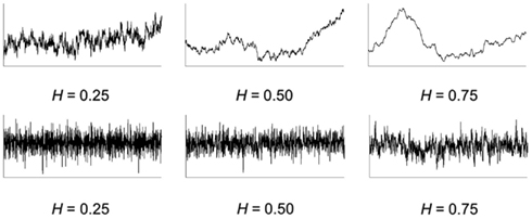
Figure 1. Top row: example series of fractional Brownian motions (fBm) for three typical values of the scaling exponent. The central graph represents an ordinary Brownian motion (H = 0.5). The left graph shows an anti-persistent fBm (H = 0.25) and the right graph a persistent fBm (H = 0.75). The corresponding fractional Gaussian noises series (fGn) are displayed in the bottom row.

Fractional Gaussian noise is defined as the series of successive increments in a fBm. In other words a fGn is the differentiation of a fBm, and conversely the integration of a fGn gives a fBm. Each fBm is then related to a specific fGn, and both are characterized by the same H exponent. We present in the bottom row of Figure 1 the fGn series corresponding to the just above fBm series. The fGn family is centered around white noise (H = 0.5), which represents the frontier between anti-persistent and persistent fGn.

These two families of processes possess fundamentally different properties: fBm series are non-stationary with time-dependent variance (diffusion property), while fGn are stationary with constant expected mean and variance over time. As previously explained, fGn and fBm can be conceived as two superimposed families, invertible in terms of differentiation and integration.

Another useful conception is to conceive these two families as representing a continuum, ranging from the most anti-persistent fGn to the most persistent fBm. This fGn/fBm continuum is characterized by the presence of scaling laws that could be expressed in the frequency or in the time domain. In the frequency domain, a scaling law relates power (i.e., squared amplitude) to frequency according to an inverse power function, with an exponent β:

$S\left(f\right)\propto \frac{1}{f^{\beta }}$ (3)

This scaling law is exploited by the Power Spectral Density (PSD) method that reveals β as the negative of the slope of the log–log representation of the power spectrum (Figure 2). The fGn/fBm continuum is then characterized by exponents β ranging from −1 to 3 (see Figure 4).

FIGURE 2

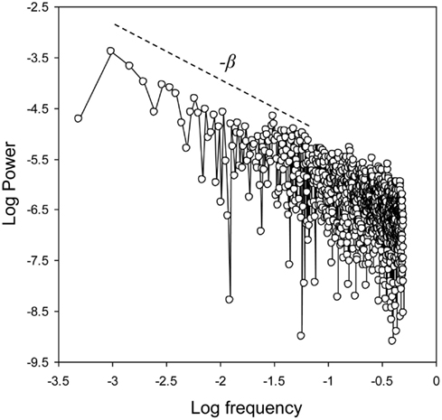
Figure 2. Power Spectral Density analysis. The exponent β is given by the negative of the slope of the log–log representation of the power spectrum.

In the time domain, the typical scaling law states that the standard deviation of the integrated series is a power function of the time over which it is computed, with an exponent α. Considering a time series x(i):

$\left\{\begin{array}{c}y\left(i\right)=\sum _{k=0}^{i}x\left(k\right)\hfill \\ \text{SD}\left(y\right)\propto n^{\alpha }\hfill \\ \hfill \end{array}\right.$ (4)

This scaling law is exploited by the Detrended Fluctuation Analysis (DFA) that reveals α as the slope of the log–log diffusion plot (Figure 3). The fGn/fBm continuum is characterized by exponents α ranging from 0 to 2 (see Figure 4). Note that the scaling law expressed in Eq. 4 just derives from the original definition of fBm (Eq. 1). If the series x(i) is a fGn, y(i) is the corresponding fBm and α is the Hurst exponent. If x(i) is a fBm, y(i) belongs to another family of over-diffusive processes, characterized by exponents α ranging from 1 to 3, and in that case α = H + 1.

FIGURE 3

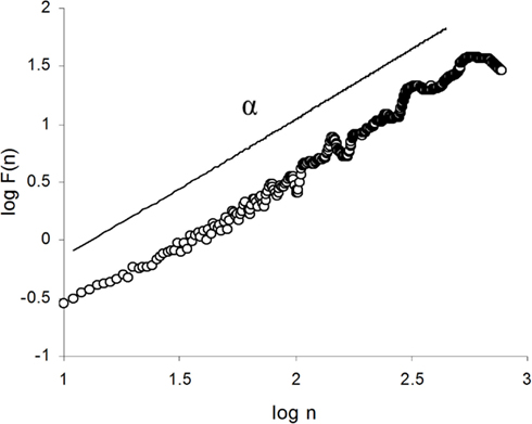
Figure 3. Detrended Fluctuation Analysis. The exponent α is determined as the slope of the log–log diffusion plot.

The different exponents that characterize these scaling laws are mutually linked by very simple equations:

For fGn series:

$\beta =2H-1\text{and}\alpha =H$ (5)

For fBm series:

$\beta =2H+1\text{and}\alpha =H+1$ (6)

For fGn and fBm series:

$\beta =2\alpha -1\text{or}\alpha =\frac{\left(\beta +1\right)}{2}$ (7)

The exponents provided by PSD and DFA (β and α, respectively), are useful because they allow to unambiguously distinguish between fGn and fBm series, which could be characterized by the same H exponents.

In this fGn/fBm continuum, LRC are generally considered to appear in a narrow range, between β = 0.5 and β = 1.5 (i.e., between α = 0.75 and α = 1.25, see Wagenmakers et al., 2004). This range is centered on β = α = 1, corresponding to the ideal 1/f noise. Long-range correlated series present typical fluctuations, often referred to as 1/f fluctuations, characterized by multiple interpenetrated waves. As can be seen in Figure 4, with the increase of the scaling exponent (α or β), the series becomes smoother and less stationary. Within this continuum, LRC series are characterized by a weak stationarity, and a median level of roughness.

FIGURE 4

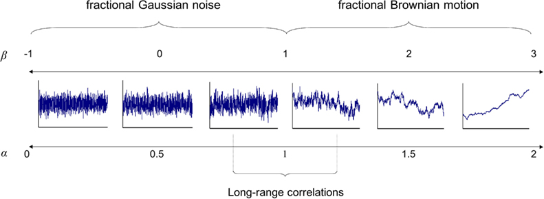
Figure 4. Representation of the fGn/fBm continuum. The continuum is characterized by exponents β ranging from −1 to 3, and by exponents α ranging from 0 to 2. White noise corresponds to β = 0 and α = 0.5, and Brownian motion to β = 2 and α = 1.5. Long-range correlations are considered to appear between β = 0.5 and β = 1.5. β = α = 1 corresponds to ideal 1/f noise.

A Index of Relative Roughness

As previously stated, our aim in this paper is to provide researchers with some indications for assessing the suitability of the monofractal model for a given time series. A number of procedures can be proposed, often complex and time-consuming. We think, however, that the property of roughness, previously evoked, could support a very simple and easily computable index for testing this suitability.

Roughness has been extensively used for characterizing the texture of surfaces (Thomas, 1999). In this context, roughness can be quantified by the deviations of a real surface from its ideal form. If deviations are large, the surface is rough, and the surface is smooth if deviations are small. A number of roughness parameters have been proposed, for example the Mean Roughness, defined as the arithmetic average of the absolute values of the deviations from the ideal surface, or the Root Mean Square Roughness, defined as the root mean square average of these deviations.

In the domain of time series analysis, roughness refers to the level of short-term irregularity in the evolution of the series. As previously proposed, roughness appears as a typical property of 1/f fluctuations, and we think that it could be useful for assessing the suitability of the monofractal model for a given series.

Roughness in a series can be assessed by the computation of local variance (Madison et al., 2009). Local variance can be defined as the variability between adjacent points in the series. This source of variance in a series is independent on others typical sources, such as long-term drifts (Madison et al., 2009), or more local trends induced by serial correlations (Torre and Balasubramaniam, 2011).

An easy way for estimating local variance is to compute the variance of the series of increments in the original series (Torre and Balasubramaniam, 2011). Some other estimates have been proposed: for example Ogden and Collier (2002) and Madison et al. (2009) assessed local variance through the average of the squared differences between adjacent values, and Delignières et al. (2004) used the average of the absolute differences between adjacent values. Despite some algorithmic divergences, all these measures provide equivalent measures of local variability, in terms of variance or standard deviation.

Local variance, however, cannot in isolation provide a relevant indication for the suitability of the monofractal model. As previously stated, local variance is independent on the strength of serial correlations in the series: similar patterns of correlation can be obtained with different levels of local variance, and conversely identical levels of local variance could appear in series possessing different levels of serial correlation (Torre and Balasubramaniam, 2011). The problem is to assess the relative contribution of local variance to the global variance of the series. In this aim, we propose an index of relative roughness (RR), defined as the ratio between local variance and global variance.

Consider a series (x_i). Local variance (LVar) can be expressed as:

$\text{LVar}\left(x_i\right)=\text{Var}\left(x_i-x_{i-1}\right)=2\left[\text{Var}\left(x_i\right)-{\gamma }_1\left(x_i\right)\right]$ (8)

γ₁(x_i) representing the lag-one autocovariance. One can then obtain the following expression for RR:

$\text{RR}=2\left[1-\frac{{\gamma }_1\left(x_i\right)}{\text{Var}\left(x_i\right)}\right]$ (9)

This equation suggests that for a white noise process, local variance should be twice the global variance, and RR should equal 2. One could also expect a progressive decrease of RR with the increase of serial correlations in the series. Finally, the diffusion property suggests that for fBm series global variance increases with series length. As a consequence, for fBm series RR should decrease as series length increases.

In order to analyze the evolution of RR according to the strength of serial correlations in the series, we generated exact fractal series with α exponents ranging from 0.1 (highly anti-persistent fGn) to 1.9 (highly persistent fBm), by steps of 0.1, using the algorithm proposed by Davies and Harte (1987). In order to check the effect of series length on RR, we worked on series of 512, 1024, and 2048 data points, which correspond to the series lengths mostly used in the literature. One-hundred series was generated for each α level and each series length. The results are illustrated in Figure 5. As expected RR decreased as correlations increased in the series. RR was about 2.0 for white noise, and anti-persistent fGn series were characterized by values greater than 2.0, up to 2.9 for the most negatively correlated series (α = 0.1). For fBm series RR presented an asymptotical trend toward zero as α increased. As expected, series length affects RR, but this effect is located in a narrow range of anti-persistent fBm (between α = 1.0 and α = 1.4).

FIGURE 5

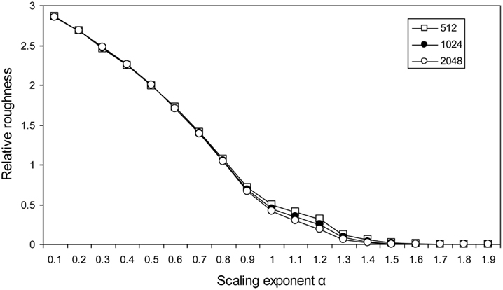
Figure 5. Relative roughness as a function of the scaling exponent α in simulated fGn and fBm series. Results are given for series lengths of 512, 1024, and 2048 data points.

We present in Table 1 the details of the results for the range 0.5–1.5. We obtained for 1/f series (α = 1.0) a mean RR ranging from 0.4 to 0.5, depending of series length. On the basis of these results, it is possible to roughly estimate the limits of the range of RR values that corresponds to the series that are usually considered as long-range correlated (0.75 < α < 1.25). For series of 512 points, RR should be approximately comprised between 1.24 and 0.28, for series of 1024 points between 1.24 and 0.17, and for series of 2048 points between 1.21 and 0.12. Note that these values should certainly not be considered as strict and absolute boundaries. The present results are dependent on the method we used to generate series, and another method would have given slightly different values.

TABLE 1

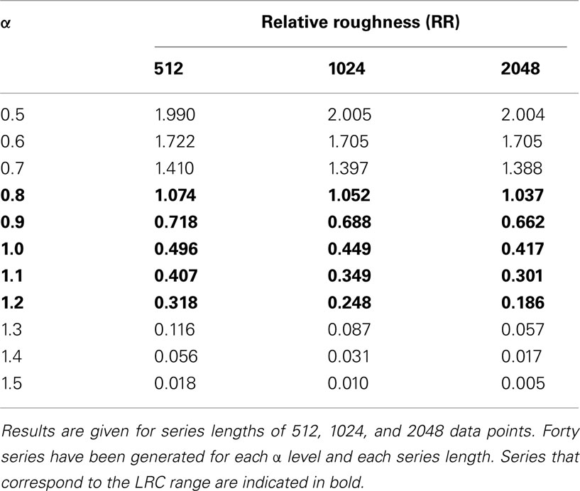
Table 1. Mean relative roughness (RR), computed for exact fractal series with α exponents ranging from 0.5 to 1.5.

Relevant Series for Fractal Analysis: Relative Phase in Bimanual Coordination Tasks

The aim of RR is to provide an easily computable index for testing the a priori suitability of the monofractal model. We think that this index could be useful for distinguishing the variables that could be relevant for the application of fractal analyses, and those that clearly fall out of the scope of the monofractal model.

An interesting example can be proposed on the basis of studies that analyzed the fractal properties of series collected in bimanual coordination tasks. In the bimanual coordination paradigm, participants are requested to perform simultaneous rhythmical oscillations with the two hands, according to a prescribed phase relationship between the two effectors (Kelso, 1984). Two modes of coordination have been shown to be particularly stable: the in-phase coordination, in which homologous muscles perform simultaneous contractions, and the anti-phase coordination, in which homologous muscles perform alternate contractions. The relevant variable for analyzing such coordination is the relative phase, i.e., the difference between the instantaneous phases of each oscillator. Relative phase equals 0° for the in-phase mode, and 180° for the anti-phase mode.

Two measures of relative phase are used in the literature, and are generally considered as interchangeable. Continuous relative phase (CRP) is derived from the position (x_t) and velocity (x_t) time series of each oscillator. The phase angle is determined for each oscillator using the following equation:

${\text{ϕ}}_t={tan}^{-1}\left(\frac{{ẋ}_t}{x_t}\right),$ (10)

and the relative phase is determined as the instantaneous difference between the phase of each oscillator.

Discrete relative phase (DRP) is punctually computed, as the temporal difference between similar inflection points in the oscillation of the two oscillators, reported to the period of one of the oscillators. CRP has often been interpreted as a higher resolution form of DRP. Nevertheless, Peters et al. (2003) showed that these two measures essentially differ in nature: DRP yields information regarding the relative dispersion of events in oscillatory signals, while CRP described their relationship in a higher order phase space.

Torre et al. (2007a) analyzed the fractal properties of both DRP and CRP series. Two example series, collected in trials performed in in-phase mode, are presented in Figure 6 (top row). At first glance, the two series look similar, presenting a weak stationarity around a mean value of 0°. However, the DRP series (left graph) contains only 1044 data points, while the CRP series is composed of 32,000 data points (sampled at 100 Hz, representing approximately 96 consecutive cycles). The graphs in the second row highlight the differences between the two series, by focusing on 200 points for DRP and 2000 points for CRP. The DRP series is composed of discrete points, and differences between adjacent values provide the series with a marked level of roughness. In contrast the CRP series appears as a very smooth motion, with slow oscillations around the mean value.

FIGURE 6

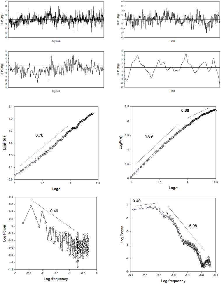
Figure 6. Top Row: relative phase series collected during a bimanual coordination task. The task was performed following an in-phase mode. The left graph represents a series of discrete relative phases (DRP, 1044 data points, computed by the point estimate method at the time of maximal pronation of the right hand). The right graph is a series of continuous relative phase (CRP, 32,000 data points, sampled at 100 Hz, representing approximately 96 consecutive cycles). Second row: DRP (left) and CRP (right) series. These graphs focus on 200 points for DRP and 2000 points for CRP. Third row: average DFA diffusion plots obtained for DRP (left), and CRP (right) series. Bottom row: average log–log power spectra obtained for DRP (left), and CRP (right) series.

Relative roughness, averaged over 12 series composed of the 2048 first points of the experimental data, was about 1.22 (±0.44) for DRP, and 0.0015 (±0.000) for CRP. These results suggest that DRP series could be reasonable candidates for being modeled as fGn processes, while CRP series appear clearly out of the range of RR values expected for LRC processes.

These results are confirmed by the application of DFA and PSD. DRP series yielded a mean α exponent of 0.76 (±0.12). The mean β was 0.49 (±0.15), corresponding according to Eq. 7 to a α value of about 0.75. These values converge toward the characterization of DRP series as weakly persistent fGn series. The analysis of CRP series provided completely different results. When computed over the whole range of intervals, the mean α was of about 1.25 (±0.11). However, a close examination of the diffusion plot (see Figure 6) revealed a clear inflection, with a steeper slope of about 1.89 (±0.03) for short time intervals, and a flattened slope (0.69 ± 0.41) for long intervals. PSD yielded a mean log–log power spectrum that also presented an inflection, with a positive mean slope of about 0.40 (±1.58) in the very low frequency region, and a highly negative slope (−5.08 ± 0.28) in the medium to high-frequency region. This last result was consistent with that reported by Schmidt et al. (1991), which obtained very high β exponents for CRP series. One could question, however, the relevancy of computing an exponent on the basis on the average slope of this kind of spectrum. An interesting point here is the discrepancy between the results obtained in the time domain (DFA) and the frequency domain (PSD). According to Rangarajan and Ding (2000), such a discrepancy should lead researchers to doubt of the genuine presence of LRC in the analyzed series.

The Special Case of Bounded Series

Another problem that could prevent the application of the monofractal model is the fact that series could appear bounded within physiological or biomechanical limits. The monofractal model suggests that fBm series are typically unbounded. The diffusion over time of a pure fBm is theoretically unlimited: fluctuations grow as a power function of time, and the expected displacement of the process from a given origin is likely to increase indefinitely.

When a series is bounded within physiological boundaries, the diffusion process is obviously limited and variance cannot exceed a ceiling value. In other words, variance is likely to become independent on time beyond a critical time interval necessary for reaching this ceiling value.

This problem was recently considered by Delignières et al. (2011a), in the domain of postural control. Research on postural control focuses on the analysis of center-of-pressure (COP) trajectory, easily recorded with force platforms. A number of authors, during the last decade, have proposed to apply to these data diverse non-linear methods, including fractal analyses. Delignières et al. (2011a) formulated strong reserves about the suitability of the fractal framework for modeling COP data, which appear clearly bounded within functional limits. Interestingly, they showed that bounding affected primarily COP velocity, rather than COP position series, as generally accepted in the literature (Collins and De Luca, 1993). This result suggested that bounding could be due to motor control limitations, rather than by biomechanical constraints as commonly assumed. We present in Figure 7 (top row) an example COP velocity series, sampled at 40 Hz, that illustrates this bounding phenomenon: COP velocity presents highly persistent trends on the short-term, but these trends tend to reverse in direction when velocity reaches the upper or the lower limits represented by the dashed lines.

FIGURE 7

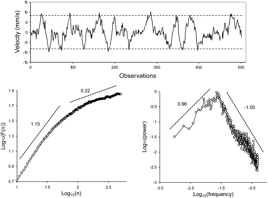
Figure 7. Top: an example series of center-of-pressure velocity, during the maintenance of upright posture (sampling frequency: 40 Hz). The dashed lines represent the upper and lower limits that bound the evolution of the series. Bottom: average DFA diffusion plot (left) and average log–log power spectrum (right). From Delignières et al. (2011a).

The presence of persistent trends on the short-term suggests a rather low roughness, similar to that observed for persistent fBm series. However, the ceiling effect on global variance yields surprising results: The computation of RR for 26 experimental series of COP velocity of 2048 data points gave a mean value of about 1.64 (±0.66), corresponding the value expected for weakly persistent fGn series (see Figure 5).

Liebovitch and Yang (1997) analyzed the effect of bounding on the results produced by fractal analyses. Especially, the diffusion plot obtained with the application of DFA is supposed in that case to present a typical inflection, with a steep slope for short time intervals revealing the persistence of the process on the short-term, and a flattening of the slope for long time intervals, due to the limitation of diffusion. The application of DFA on the series of COP velocity clearly illustrate this crossover (see Figure 7): the diffusion plot presents a slope of about 1.0 for short time intervals, and a slope of 0.43 for long intervals. Note that the crossover can also be revealed by PSD: the log–log power spectrum presents a marked inflection, with a positive slope in the low frequency region revealing negative correlations on the long-term, and a negative slope in the high-frequency region, due to the persistent trends on the short-term (Figure 7, bottom row, right column).

The application of fractal-like methods to bounded series has sometimes lead to interpretations in terms of dual fractal regime, with a persistent behavior on the short-term and an anti-persistent behavior on the long-term (e.g., Collins and De Luca, 1993; Treffner and Kelso, 1995, 1999). In the present case a simpler hypothesis related to the effect of bounding on the dynamics of the variable under study, offers a more interesting and useful interpretation.

Discrepancies between Relative Roughness and Scaling Exponents

The previous examples showed how the measure of RR could allow to a priori assessing the plausibility of the fractal hypothesis. When RR is clearly out of the range expected for LRC, the reference to the monofractal framework can be abandoned.

Relative roughness, however, is not sufficient for unambiguously characterizing a given series as long-range correlated. In others words, a series can present a level of RR located in the range expected for LRC processes, without being actually long-range correlated.

In order to illustrate this problem, we simulated three sets of time series, possessing different correlation properties. The first set was generated by a one-order auto-regressive model:

$y_i=\phi y_{i-1}+{\epsilon }_i$ (11)

In this equation Φ is the auto-regressive parameter and was set to 0.85. ε_i is a white noise process with zero mean and unit variance. The second set was generated by an integrated one-order moving average model:

$y_i=y_{i-1}-\theta {\epsilon }_{i-1}+{\epsilon }_i$ (12)

In this equation θ is the first-order moving average parameter and was set to 0.8. ε_i is a white noise process with zero mean and unit variance. Finally we used the Davies–Harte algorithm for simulating a set of fractional Gaussian noise series, with H = 0.9 (Davies and Harte, 1987). Each set was composed of 100 series of 1024 points. By construction, the two first sets of series present only short-term correlations, while the third one possesses LRC properties.

We choose these ARMA models and their parameters values because the application of DFA on the series generated by these models yields diffusion plots similar to those obtained with fGn series. We present in Figure 8 one example series of each set, and the corresponding diffusion plots: in all cases a linear slope close to 0.9 is obtained. Obviously the best linear fit is observed for the fGn series, which contains genuine LRC. For the AR series, the diffusion plot presents a slight flattening for long intervals, and conversely the slope tends to increase for long intervals for the MA series. However the diffusion plots obtained the AR and MA series roughly mimic the typical shape expected from long-range correlated series, and could easily lead to erroneous interpretations.

FIGURE 8

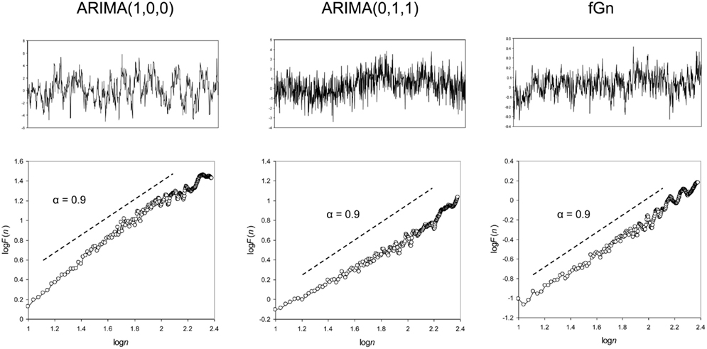
Figure 8. Top row: example series simulated with a one-order auto-regressive model (y_i = 0.85y_{i − 1} + ε_i, left column), a one-order moving average model (y_i = y_{i − 1} – 0.8ε_{i − 1} + ε_i, central column), and the Davies–Harte algorithm (fGn with H = 0.9, right column). The corresponding DFA diffusion plots are presented in the bottom row.

More precisely, considering the 100 series of each set, the mean α exponent was 0.92 ± 0.06 for AR series, 0.92 ± 0.08 for MA series, and 0.90 ± 0.07 for fGn series. In contrast, the computation of RR gave different values in the three sets: the mean RR was 0.30 ± 0.03 for AR series, 0.87 ± 0.36 for MA series, and 0.69 ± 0.09 for fGn series. For fGn series, the mean RR corresponded exactly to the expected value (see Table 1). With respect to the obtained α exponent, AR series were characterized by a mean RR value lower than expected, and conversely for MA series RR was slightly higher than expected.

Such discrepancies between the expected and obtained RR values could represent an interesting test for the suitability of the monofractal model. Note, however, that these differences between expected and obtained values should be considered with some caution. The mean RR value of 0.30 obtained for AR series corresponds to the expected value for fBm series with α = 1.1, and the mean value of 0.83 obtained for MA series to the expected value for fGn series with α = 0.8. Considering the possible error in the estimation of α, especially for relatively short series (see Delignières et al., 2006), the discrepancy between α and RR should be only considered one indicator, among others, for characterizing the series.

Some methods have been especially developed for distinguishing between short-term and LRC. Wagenmakers et al. (2005) and Torre et al. (2007b) have proposed a method based on ARMA and ARFIMA modeling. This method consists in fitting 18 models to the series. Nine of these models are ARMA (p, q) models, p and q varying systematically from 0 to 2. These ARMA models do not contain any long-range serial correlations. The other nine models are the corresponding ARFIMA (p, d, q) models, differing from the previous ARMA models by the inclusion of the fractional integration parameter d representing persistent serial correlations. One supposes that if the analyzed series contains LRC, ARFIMA models should present a better fit than their ARMA counterparts. We applied the ARMA/ARFIMA modeling to the three sets of series: as expected, all series in the fGn set were recognized as long-range correlated. In contrast, only 10% of the AR series and 14% of the MA series were best fitted by ARFIMA models.

Note that Gilden (2009) has issued severe reservations against methods based on goodness-of-fit criteria, such as the ARMA/ARFIMA procedure proposed by Wagenmakers et al. (2004). As an alternative, the author proposed global analyses that evaluate models on the basis of their capacity of generalization. The models are examined in terms of cross-validity, flexibility, and representativeness.

One could wonder about the added value of the proposed RR index, with regard to these methods that allow to detect the genuine presence of LRC in data sets. RR just provides an a priori indication about the possible relevancy of the monofractal model, but is unable to attest for the genuine presence of LRC. One could propose to systematize the application the aforementioned methods before any consideration of the fractal approaches. However it is clear that these methods are rarely used in the litterature. These methods remain complex to implement, and their theoretical backgrounds are sometimes difficult. Often authors prefer to directly apply fractal methods such as PSD or DFA, and to interpret a posteriori the obtained results. The RR index presents the advantage to be very easy to compute, and can allow avoiding superfluous investigations.

Time Series and Event Series

The two first examples we evoked in this paper (relative phase series and COP velocity) open an interesting line of discussion about the relevancy of fractal analyses. One could note that in both cases the series that appear unsuitable for being modeled through the monofractal framework were genuine time series, i.e., series of successive values spaced by equal time intervals.

In contrast, DRP series correspond to a cycle-to-cycle measurement, and the time interval between two successive values depends on the local period used as denominator in the calculation of relative phase. DRP series are just event series, composed of temporally ordered measures, but cannot be considered genuine time series. It is important to note that in most cases, experiments that clearly evidenced the presence of fractal fluctuations did not consider time series but event series. This was the case, for example, for the inter-tap intervals series in finger tapping experiments (Gilden et al., 1995; Lemoine et al., 2006), or for the stride intervals series analyzed in walking experiments (Hausdorff et al., 1995, 1997). In the set of experiments proposed by Gilden (2001), all analyzed series were as well composed of ordered successive performances.

At a methodological level, this could be considered an obstacle for the application of time series analyses such as those previously presented. Is it possible to apply analyses dealing with notions such as frequency or time intervals with data series where time is not effectively present? The application of time series analyses to event series is generally accepted pending some theoretical adaptations. Obviously, when dealing with an event series, time cannot be considered in its absolute sense. When applying PSD, “frequency” should not be read in Hertz units, but rather in terms of inverse trial number (Gilden, 2001), or in number of cycles for N trials or observations (Musha et al., 1985; Yamada, 1996). As well, the “intervals” taken into account by DFA are not genuine time intervals, but rather lengths of samples of successive observations.

This distinction between time series and event series is a key point in fractal analyses. Researchers aiming at undertaking a fractal approach to a given system could be naturally inclined to opt for time series, considering the nature of the statistical procedures commonly used in this domain. However, we think that the key variable in fractal analysis is not fluctuation in time, but rather cycle-to-cycle or trial-to-trial fluctuation. As argued by Kello et al. (2007), 1/f fluctuations are likely to occur when a system is repeatedly exposed to the same set of constraints. Gilden (2001) developed a similar idea, suggesting that the emergence of 1/f fluctuations is dependent on the consistency of the mental set, i.e., the reproducibility of constraints over successive trials. When a system has to repeatedly produce the same performance in the same situation, fluctuations in performance are likely to reveal its constitutive complexity. Essential properties of complex systems, such as degeneracy, suggest that the neural networks that are in charge of the production of performance are never identical from one trial to the other, but are never completely different. This capacity to mobilize softly assembled and evolving networks over successive trials could be considered the essential origin of LRC in the series of performances produced by complex systems (Delignières et al., 2011b).

Note, however, that the collection of event series is often difficult and time-consuming. The successive performance of hundreds of trials on a given task raises evident methodological problems and experimental biases, related to fatigue, or motivation. In contrast, the collection of time series, especially with high-frequency recording devices, could appear easier. Obviously, we do not argue that fractal analyses cannot be applied on genuine time series. Some convincing experiments have been published that were based on the analysis of time series, for example in the study of force production (Sosnoff and Newell, 2005), or electroencephalographic data (Nikulin and Brismar, 2004). In these examples, however, series were recorded from systems in steady state condition, and the successive measurements are likely to represent ordered assessments of a more or less stationary variable. In contrast, in a number of situations time series represent a kind of displacement in a given physical environment (for example COP trajectories) or in a more formal space (for example CRP series). Obviously, such series tend to present strong persistent correlations between successive positions, and this kind of motion falls clearly out of the scope of LRC processes. A solution in this case can be to seek for LRC properties in the series of successive increments, rather than in the original series (see, for example, Stephen et al., 2010).

Conclusion

Long-range correlations remain a very intriguing phenomenon, and the recent theoretical advances in this domain suggest that these fluctuations could represent a key entry in the study of the functional complexity of living systems. However, if the presence of serial correlations in series of data collected on such systems is surely more the rule than the exception (Slifkin and Newell, 1998), this does not imply that these correlations possess long-range properties. The RR index we discussed in this paper represents a simple tool allowing an easy prior assessment of the plausibility of the LRC hypothesis for a given series. We showed, however, that additional precautions are necessary in order to avoid erroneous conclusions or interpretations.

Note, however, that if the RR index can serve as an a priori warning light, some options can be considered before the definitive abandon of the monofractal framework. As previously suggested, one can often choose alternative variables that are better suitable for fractal analyses (e.g., DRP rather than CRP). Series transformations, by means of differentiation or integration, can also be used for obtaining more relevant data sets. Finally series are often contaminated by trends, caused by external effects, that could spuriously increase global variance, with respect to the amplitude of local fluctuations. In those cases RR could appear very low and lead to rejection of the monofractal hypothesis. Modified versions of the DFA, including polynomial detrending of various orders, have been proposed for controlling this kind of non-stationarities (Kantelhardt et al., 2001). When series are definitively too smooth for being accounted for by the monofractal model, one could consider other methods, based on phase space reconstruction, and especially Recurrence Analysis that allows revealing hidden regularities in apparently unpredictable signals (Webber and Zbilut, 2005).

Long-range correlations have recently become a very popular theme of research. A number of researchers have tried to check whether their usual objects of research could present LRC properties. However, we think that evidencing the presence of LRC in a given system cannot represent per se an interesting research goal. The problem is not to seek everywhere for LRC, but to determine, theoretically, where it could be important, and empirically where it could be plausible to find such long-term persistent serial correlations.

Conflict of Interest Statement

The authors declare that the research was conducted in the absence of any commercial or financial relationships that could be construed as a potential conflict of interest.

References

Collins, J. J., and De Luca, C. J. (1993). Open-loop and closed-loop control of posture: a random-walk analysis of center-of-pressure trajectories. Exp. Brain Res. 95, 308–318.

Pubmed Abstract | Pubmed Full Text | CrossRef Full Text

Davies, R. B., and Harte, D. S. (1987). Tests for Hurst effect. Biometrika 74, 95–101.

CrossRef Full Text

Delignières, D., Fortes, M., and Ninot, G. (2004). The fractal dynamics of self-esteem and physical self. Nonlinear Dynamics Psychol. Life Sci. 8, 479–510.

Pubmed Abstract | Pubmed Full Text

Delignières, D., Ramdani, S., Lemoine, L., Torre, K., Fortes, M., and Ninot, G. (2006). Fractal analysis for short time series: a reassessment of classical methods. J. Math. Psychol. 50, 525–544.

CrossRef Full Text

Delignières, D., Torre, K., and Bernard, P. L. (2011a). Transition from persistent to anti-persistent correlations in postural sway indicates velocity based control. PLoS Comput. Biol. 7, e1001089. doi:10.1371/journal.pcbi.1001089

CrossRef Full Text

Delignières, D., Marmelat, V., and Torre, K. (2011b). “Degeneracy and long-range correlation: a simulation study,” in Proceeding BIO Web of Conferences 1, Montpellier, 00020.

Gilden, D. L. (1997). Fluctuations in the time required for elementary decisions. Psychol. Sci. 8, 296–301.

CrossRef Full Text

Gilden, D. L. (2001). Cognitive emissions of 1/f noise. Psychol. Rev. 108, 33–56.

Pubmed Abstract | Pubmed Full Text | CrossRef Full Text

Gilden, D. L. (2009). Global model analysis of cognitive variability. Cogn. Sci. 33, 1441–1467.

Pubmed Abstract | Pubmed Full Text | CrossRef Full Text

Gilden, D. L., Thornton, T., and Mallon, M. W. (1995). 1/f noise in human cognition. Science 267, 1837–1839.

Pubmed Abstract | Pubmed Full Text | CrossRef Full Text

Goldberger, A. L., Amaral, L. A. N., Hausdorff, J. M., Ivanov, P. Ch., Peng, C.-K., and Stanley, H. E. (2002). Fractal dynamics in physiology: alterations with disease and aging. Proc. Natl. Acad. Sci. U.S.A. 99, 2466–2472.

Pubmed Abstract | Pubmed Full Text | CrossRef Full Text

Hausdorff, J. M., Mitchell, S. L., Firtion, R., Peng, C. K., Cudkowicz, M. E., Wei, J. Y., and Goldberger, A. L. (1997). Altered fractal dynamics of gait: reduced stride-interval correlations with aging and Huntington’s disease. J. Appl. Physiol. 82, 262–269.

Pubmed Abstract | Pubmed Full Text

Hausdorff, J. M., Peng, C.-K., Ladin, Z., Wei, J. Y., and Goldberger, A. L. (1995). Is walking a random walk? Evidence for long-range correlations in stride interval of human gait. J. Appl. Physiol. 78, 349.

Pubmed Abstract | Pubmed Full Text

Hurst, H. E. (1951). Long-term storage capacity of reservoirs. Trans. Am. Soc. Civil Eng. 116, 770–799.

Kantelhardt, J. W., Koscielny-Bunde, E., Rego, H. H. A., Havlin, S., and Bunde, A. (2001). Detecting long-range correlations with detrended fluctuation analysis. Physica A 295, 441–454.

CrossRef Full Text

Kello, C. T., Beltz, B. C., Holden, J. G., and Van Orden, G. C. (2007). The emergent coordination of cognitive function. J. Exp. Psychol. Gen. 136, 551–568.

Pubmed Abstract | Pubmed Full Text | CrossRef Full Text

Kelso, J. A. S. (1984). Phase transition and critical behaviour in human bimanual coordination. Am. J. Physiol. 15, R1000–R1004.

Leland, W. E., Taqqu, M. S., Willinger, W., and Wilson, D. V. (1994). On the self-similar nature of ethernet traffic (extended version). IEEE/ACM Trans. Netw. 2, 1–15.

CrossRef Full Text

Lemoine, L., Torre, K., and Delignières, D. (2006). Testing for the presence of 1/f noise in continuation tapping data. Can. J. Exp. Psychol. 60, 247–257.

Pubmed Abstract | Pubmed Full Text | CrossRef Full Text

Liebovitch, L. S., and Yang, W. (1997). Transition from persistent to antipersistent correlation in biological systems. Phys. Rev. E 56, 4557–4566.

CrossRef Full Text

Madison, G., Forsman, L., Blom, Ö., Karabanov, A., and Ullén, F. (2009). Correlations between intelligence and components of serial timing variability. Intelligence 37, 68–75.

CrossRef Full Text

Mandelbrot, B. B., and van Ness, J. W. (1968). Fractional Brownian motions, fractional noises and applications. SIAM Rev. 10, 422–437.

CrossRef Full Text

Matsuzaki, M. (1994). Fractals in earthquakes. Philos. Trans. R. Soc. Lond. A 348, 449–457.

CrossRef Full Text

Musha, T., Katsurai, K., and Teramachi, Y. (1985). Fluctuations of human tapping intervals. IEEE Trans. Biomed. Eng. 32, 578–582.

Pubmed Abstract | Pubmed Full Text | CrossRef Full Text

Nikulin, V. V., and Brismar, T. (2004). Long-range temporal correlations in alpha and beta oscillations: effect of arousal level and test–retest reliability. Clin. Neurophysiol. 115, 1896–1908.

Pubmed Abstract | Pubmed Full Text | CrossRef Full Text

Ogden, R. T., and Collier, G. L. (2002). Inference on variance components of autocorrelated sequences in the presence of drift. J. Nonparamet. Stat. 14, 409–420.

CrossRef Full Text

Peters, B. T., Haddad, J. M., Heiderscheit, B. C., van Emmerik, R. E. A., and Hamill, J. (2003). Limitation in the use and interpretation of continuous relative phase. J. Biomech. 36, 271–274.

Pubmed Abstract | Pubmed Full Text | CrossRef Full Text

Rangarajan, G., and Ding, M. (2000). Integrated approach to the assessment of long range correlation in time series data. Phys. Rev. E Stat. Phys. Plasmas Fluids Relat. Interdiscip. Topics 61, 4991–5001.

Pubmed Abstract | Pubmed Full Text | CrossRef Full Text

Schmidt, R. C., Beek, P. J., Treffner, P. J., and Turvey, M. T. (1991). Dynamical substructure of coordinated rhythmic movements. J. Exp. Psychol. Hum. Percept. Perform. 17, 635–651.

Pubmed Abstract | Pubmed Full Text | CrossRef Full Text

Slifkin, A. B., and Newell, K. M. (1998). Is variability in human performance a reflection of system noise? Curr. Dir. Psychol. Sci. 7, 170–177.

CrossRef Full Text

Sosnoff, J. J., and Newell, K. M. (2005). Intermittent visual information and the multiple timescales of visual motor control of continuous isometric force production. Percept. Psychophys. 67, 335–344.

Pubmed Abstract | Pubmed Full Text | CrossRef Full Text

Stephen, D. G., Arzamarski, R., and Michaels, C. F. (2010). The role of fractality in perceptual learning: exploration in dynamic touch. J. Exp. Psychol. Hum. Percept. Perform. 36, 1161–1173.

Pubmed Abstract | Pubmed Full Text | CrossRef Full Text

Stevens, S. S. (1951). “Mathematics, measurement and psychophysics,” in Handbook of Experimental Psychology, ed. S. S. Stevens (New York: Wiley), 1–49.

Thomas, T. R. (1999). Rough Surfaces. London: Imperial College Press.

Torre, K., and Balasubramaniam, R. (2011). Disentangling stability, variability and adaptability in human performance: focus on the interplay between local variance and serial correlation. J. Exp. Psychol. Hum. Percept. Perform. 37, 539–550.

Pubmed Abstract | Pubmed Full Text | CrossRef Full Text

Torre, K., Delignières, D., and Lemoine, L. (2007a). 1/f^β fluctuations in bimanual coordination: an additional challenge for modeling. Exp. Brain Res. 183, 225–234.

CrossRef Full Text

Torre, K., Delignières, D., and Lemoine, L. (2007b). Detection of long-range dependence and estimation of fractal exponents through ARFIMA modelling. Br. J. Math. Stat. Psychol. 60, 85–106.

CrossRef Full Text

Treffner, P. J., and Kelso, J. A. S. (1999). Dynamic encounters: long-memory during functional stabilization. Ecol. Psychol. 11, 103–137.

CrossRef Full Text

Treffner, P. J., and Kelso, J. A. S. (1995). “Functional stabilization on unstable fixed-points,” in Studies in Perception and Action III, eds B. G. Bardy, R. J. Bootsma, and Y. Guiard (Hillsdale, NJ: Laurence Erlbaum Associates), 83–86.

van Orden, G. C., Holden, J. G., and Turvey, M. T. (2003). Self-organization of cognitive performance. J. Exp. Psychol. Gen. 132, 331–350.

Pubmed Abstract | Pubmed Full Text | CrossRef Full Text

Wagenmakers, E.-J., Farrell, S., and Ratcliff, R. (2004). Estimation and interpretation of 1/f^α noise in human cognition. Psychon. Bull. Rev. 11, 579–615.

Pubmed Abstract | Pubmed Full Text | CrossRef Full Text

Wagenmakers, E.-J., Farrell, S., and Ratcliff, R. (2005). Human cognition and a pile of sand: a discussion on serial correlations and self-organized criticality. J. Exp. Psychol. Gen. 134, 108–116.

Pubmed Abstract | Pubmed Full Text | CrossRef Full Text

Webber, C. L. Jr., and Zbilut, J. P. (2005). “Recurrence quantification analysis of nonlinear dynamical systems,” in Tutorials in Contemporary Nonlinear Methods for the Behavioral Sciences, eds M. A. Riley and G. C. Van Orden 26–94. Available at: http://www.nsf.gov/sbe/bcs/pac/nmbs/nmbs.jsp (Retrieved March 2, 2011).

Yamada, M. (1996). Temporal control mechanism in equalled interval tapping. Appl. Human Sci. 15, 105–110.

Pubmed Abstract | Pubmed Full Text | CrossRef Full Text