
94% of researchers rate our articles as excellent or good
Learn more about the work of our research integrity team to safeguard the quality of each article we publish.
Find out more
METHODS article
Front. Physiol., 04 June 2012
Sec. Fractal Physiology
Volume 3 - 2012 | https://doi.org/10.3389/fphys.2012.00141
This article is part of the Research TopicFractal Analyses: Statistical and Methodological Innovations and Best Practices.View all 12 articles
A commentary has been posted on this article:
Multifractal analysis for all
Fractal structures are found in biomedical time series from a wide range of physiological phenomena. The multifractal spectrum identifies the deviations in fractal structure within time periods with large and small fluctuations. The present tutorial is an introduction to multifractal detrended fluctuation analysis (MFDFA) that estimates the multifractal spectrum of biomedical time series. The tutorial presents MFDFA step-by-step in an interactive Matlab session. All Matlab tools needed are available in Introduction to MFDFA folder at the website www.ntnu.edu/inm/geri/software. MFDFA are introduced in Matlab code boxes where the reader can employ pieces of, or the entire MFDFA to example time series. After introducing MFDFA, the tutorial discusses the best practice of MFDFA in biomedical signal processing. The main aim of the tutorial is to give the reader a simple self-sustained guide to the implementation of MFDFA and interpretation of the resulting multifractal spectra.
The structural characteristics of biomedical signals are often visually apparent, but not captured by conventional measures like the average amplitude of the signal. Biomedical signals from a wide range of physiological phenomena posses a scale invariant structure. A biomedical signal has a scale invariant structure when the structure repeats itself on subintervals of the signal. Formally, the biomedical signal X(t) are scale invariant when X(ct) = cHX(t). Fractal analyses estimates the power law exponent, H, that defines the particular kind of scale invariant structure of the biomedical signal. Fractal analyses are frequently employed in biomedical signal processing to define the scale invariant structure in ECG, EEG, MR, and X-ray pictures (cf. Lopes and Betrouni, 2009). The scale invariant structures of inter-spike-interval of neuron firing, inter-stride-interval of human walking, inter-breath-interval of human respiration, and inter-beat intervals of the human heart has differentiated between healthy and pathological conditions (e.g., Ivanov et al., 1999; Peng et al., 2002; Zheng et al., 2005; Hausdorff, 2007), and between different types of pathological conditions (e.g., Wang et al., 2007). Scale invariant structures are also found in spatial phenomena like the branching of the nervous system and lungs (e.g., Bassingthwaighte et al., 1990; Abbound et al., 1991; Weibel, 1991; Krenz et al., 1992), bone structure (Parkinson and Fazzalari, 1994), and are able to differentiate between healthy and cancer tissues (Atupelage et al., 2012). Several reports during the last decade suggest that changes in the scale invariant structure of biomedical signals reflect changes in the adaptability of physiological processes and successful treatment of pathological conditions might change fractal structure and improve health (Goldberger, 1996; Goldberger et al., 2002). Fractal analyses are therefore promising prognostic and diagnostic tools in biomedical signal processing.
Monofractal and multifractal structures of the biomedical signal are particular kind of scale invariant structures. Most commonly, the monofractal structure of biomedical signals are defined by a single power law exponent and assumes that the scale invariance is independent on time and space. However, spatial and temporal variation in scale invariant structure of the biomedical signal often appears. These spatial and temporal variations indicate a multifractal structure of the biomedical signal that is defined by a multifractal spectrum of power law exponents. As an example, age related changes in the scale invariant structure of heart rate variability are indicated by changes of the multifractal spectrum rather than a single power law exponent (e.g., Makowiec et al., 2011). The width and shape of the multifractal spectrum can also differentiate between the heart rate variability from patients with heart diseases like ventricular tachycardia, ventricular fibrillation and congestive heart failure (e.g., Ivanov et al., 1999; Wang et al., 2007). The multifractal structure of heart rate variability is therefore suggested to reflect important properties of the autonomic regulation of the heart rate (Goldberger et al., 2002). Furthermore, the multifractal spectrum of endogenous brain dynamics and response times is more sensitive to the influence of age and cognitive performance compared to a single power law exponent alone (Suckling et al., 2008; Ihlen and Vereijken, 2010). Furthermore, the multifractal structure of EEG and series of inter-spike intervals have been able to differentiate between the neural activities of brain areas (Zheng et al., 2005). Multifractal analyses might therefore be important as a computer aided tool to increase the precision of neurosurgeries. The main aim of the present tutorial is to introduce a robust analysis called the multifractal detrended fluctuation analysis (MFDFA) that can estimate the multifractal spectrum of power law exponents from a biomedical time series (Kantelhardt et al., 2002). Those readers not familiar with analysis of monofractal fluctuations in biomedical signals are referred to Eke et al. (2000).
The tutorial is intended to be a self-sustained guide to the implementation of MFDFA to time series and interpretation of the resulting multifractal spectra to the readers that are unfamiliar to fractal analysis. In order to be a self-sustained guide, the tutorial decomposes MFDFA into a series of simple Matlab codes that are introduced in a step-wise manner to the reader. The tutorial is meant to be interactive where the reader can employ the Matlab codes while reading the text to enhance the understanding of MFDFA. The reader is therefore advised to download the folder “Introduction to MFDFA” at the web site www.ntnu.edu/inm/geri/software where all Matlab codes used in the tutorial are available. The reader should set the folder as the current directory folder in Matlab before reading the following sections of the tutorial. The folder can be set as current directory folder by pasting it into the current directory window after opening Matlab. Matlab variables,
parameters, and commands are written in the Matlab command font and a red color to separate them from the rest of the text. The reader can type the red commands in the Matlab command window wherever they appear in the text to access variables and parameters or plot them with Matlab’s plot function. A translation of the Matlab codes of MFDFA to the mathematical notations used by Kantelhardt et al. (2002) are given for the readers interested in the mathematical details of the MFDFA. The rest of the tutorial is divided into two sections: the implementation of MFDFA in Matlab is introduced step-by-step in Section “Multifractal Detrended Fluctuation Analysis in Matlab” where the interpretation of the resulting multifractal spectrum is emphasized. Important issues for the best practice of MFDFA are discussed in Section “The Best Practice of Multifractal Detrended Fluctuation Analysis.”
The construction of MFDFA is divided into eight steps: Section “Noise and Random Walk Like Variation in a Time Series” introduces a method to convert a noise like time series into a random walk like time series that is a preliminary step for MFDFA. Section “Computing the Root-Mean-Square Variation of a Time Series” introduces root-mean-square (RMS) that is the basic computation within MFDFA and a typical way to compute the average variation of biomedical time series. Section “Local Root-Mean-Square Variation in the Time Series” introduces the computation of local fluctuation in the time series as RMS of the time series within non-overlapping segments. In Section “Local Detrending of the Time Series,” the same local RMS is computed around trends that are often encountered in biomedical time series. In Section “Monofractal Detrended Fluctuation Analysis,” the amplitudes of the local RMS are summarized into an overall RMS. The overall RMS of the segments with small sample sizes is dominated by the fast fluctuations in the time series. In contrast, the overall RMS for segments with large sample sizes is dominated by slow fluctuations. The power law relation between the overall RMS for multiple segment sample sizes (i.e., scales) is defined by a monofractal detrended fluctuation analysis (DFA) and is called the Hurst exponent. In Section “Multifractal Detrended Fluctuation Analysis of Time Series,” MFDFA is obtained by the q-order extension of the overall RMS. The q-order RMS can distinguish between segments with small and large fluctuations. The power law relation between the q-order RMS is numerical identified as the q-order Hurst exponent. In Section “The Multifractal Spectrum of Time Series,” several multifractal spectra are computed from the q-order Hurst exponent. In Section “A Direct Estimation of the Multifractal Spectrum,” an alternative version of MFDFA is introduced that compute the multifractal spectrum directly from the local fluctuations without the q-order overall RMS.
Before starting the introduction of MFDFA, the reader can type load fractaldata.mat in the Matlab command window to access the time series, whitenoise, monofractal, and multifractal. These time series will be used as test series in the rest of Section “Multifractal Detrended Fluctuation Analysis in Matlab” while constructing MFDFA piece-by-piece. The construction of the Matlab code for MFDFA is represented as Matlab code boxes within the text. The main intention of these Matlab code boxes is that the reader should paste the Matlab code into the Matlab command window while reading the tutorial. Figures are accessed by typing the plot command at the end of the Matlab code boxes. The reader can access all Matlab code boxes by opening the m-file Matlabcodes contained in the “Introduction to MFDFA” folder.
The red traces in Figure 1 show an ordinary random walk (lower panel), a monofractal random walk (middle panel) and a multifractal random walk (upper panel). The fractal property of these random walks is reflected by their picture-in-picture similarity as illustrated in the upper panel of Figure 1. Small “hills” and “valleys” with similar structure appear when you zoom on the large “hills” and “valleys” of the random walk. The DFA is employed to time series with a random walk like structure (Peng et al., 1995). However, most biomedical time series have fluctuations that are more similar to the increments of the random walks (see the blue traces in Figure 1). If the biomedical time series has the noise like structure of the blue traces in Figure 1, it should be converted to a random walk like time series before employing DFA. Noises can be converted to random walks by subtracting the mean value and integrate the time series. Time series whitenoise, monofractal, and multifractal are all noise like time series and are converted to random walk like time series by Matlab code 1 below:
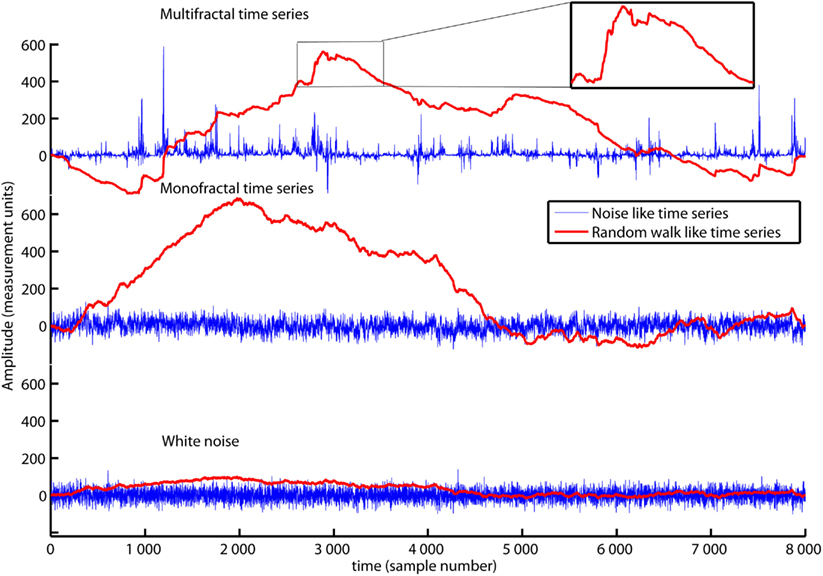
Figure 1. The time series multifractal (upper panel), monofractal (middle panel), and whitenoise (lower panel) are shown as blue traces. They are examples of noise like time series used in the present tutorial. All time series contain 8000 data samples each where the sample numbers are indicated by the horizontal axis. Matlab code 1 converts the noises (blue traces) to random walks (red traces) that have a picture-in-picture similarity (subplot in the upper panel). Notice that the time series multifractal has distinct periods with small and large fluctuations in contrast to time series monofractal and whitenoise. The aim of this section is to introduce MFDFA that quantify the structure of fluctuations within the periods with small and large fluctuations.
Matlab code 1:
RW1=cumsum(whitenoise-mean(whitenoise));

RW2=cumsum(monofractal-mean(monofractal));

RW3=cumsum(multifractal-mean(multifractal));
Type plot1 in the command window to access Figure 1.
A conventional analysis of variation in biomedical time series is to compute the average variation as a RMS. The reader can use Matlab code 2 below to compute RMS for the time series whitenoise, monofractal, and multifractal:
Matlab code 2:
RMS_ordinary=sqrt(mean(whitenoise.^2));

RMS_monofractal=sqrt(mean(monofractal.^2));

RMS_multifractal=sqrt(mean(multifractal.^2));
Type plot2 in the Matlab command window to access Figure 2.
Figure 2 illustrates that the average amplitude of variation (i.e., RMS) is equal for all three time series, whitenoise, monofractal, and multifractal, even though they have quite different structures. MFDFA will be able to distinguish between these structures as we will see in the sections below.
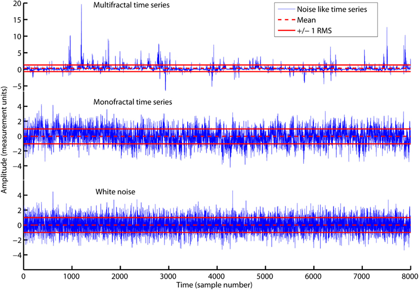
Figure 2. The time series multifractal (upper panel), monofractal (middle panel), and whitenoise (lower panel) with zero average (red dashed lines) and ±1 RMS (red solid lines). All time series have equal RMS = 1, but quite different structure. RMS is only sensitive to differences in the amplitude of variation and not differences in the structure of variation. Notice the different scaling for the vertical axis of the multifractal time series.
The multifractal time series in the upper panel have local fluctuations with both large and small magnitudes. RMS in Matlab code 2 can be computed for segments of the time series to differentiate between the magnitudes of the local fluctuations. A simple procedure is to cut the time series into equal-sized non-overlapping segments and compute a local RMS for each segment. This can be done by Matlab code 3 below and is the core procedure of MFDFA:
Matlab code 3:
X=cumsum(multifractal-mean(multifractal));

X=transpose(X);

scale=1000;

m=1;

segments=floor(length(X)/scale);

for v=1:segments

  Idx_start=((v-1)*scale)+1;

  Idx_stop=v*scale;

  Index{v}=Idx_start:Idx_stop;

  X_Idx=X(Index{v});

  C=polyfit(Index{v},X(Index{v}),m);

  fit{v}=polyval(C,Index{v});

  RMS{1}(v)=sqrt(mean((X_Idx-fit{v}).^2));

end
Type plot3 in Matlab command window to access Figure 3.
The first line of Matlab code 3 converts the noise like time series, multifractal, to a random walk like time series X (i.e., Matlab code 1). The third line of Matlab code 3 set the parameter scale that defines the sample size of the non-overlapping segments in which the local RMS, RMS{1}, are computed. The fifth line is the number of segments that the time series X can be divided into where length(X) is the sample size of time series X. Thus, segments = 8 when length(X) = 8000 and scale = 1000. The sixth to fourteenth line is a loop that computes the local RMS around a trend fit{v} for each segment by updating the time Index (see red v arguments in Matlab code 3). In the first loop v = 1, the Index{1} goes from sample 1 to sample 1000. In the second loop v = 2, the Index{2} goes from sample 1001 to sample 2000. In the final loop v = 8, the Index{8} goes from sample 7001 to 8000.
Slow varying trends are present in biomedical time series and detrending of the signal is therefore necessary to quantify the scale invariant structure of the variation around these trends. In Matlab code 3, a polynomial trend fit{v} is fitted to X within each segment v (see blue command lines in Matlab code 3). The first blue command line is the parameter m that defines the order of the polynomial. The polynomial trend are linear when m = 1, quadratic when m = 2, and cubic when m = 3 (see Figures 3A–C). The first blue command line within the loop defines the polynomial coefficients C used to create the polynomial trend fit{v} of each segment (see dashed red lines in Figure 3). The local fluctuation, RMS{1}(v), is then computed for the residual variation, X(Index{v})-fit{v}, within each segment v. The local fluctuation, RMS{1}(v), is illustrated in Figure 3 as the distance between the red dashed trends and the red solid lines.
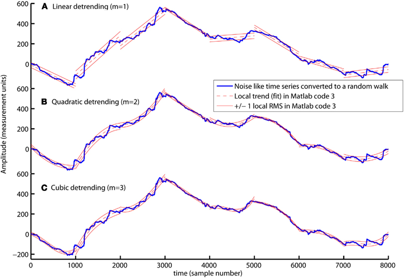
Figure 3. The computation of local fluctuations, RMS{1}, around linear (A), quadratic (B), and cubic trends (C) by Matlab code 3 (m = 1, m = 2, and m = 3, respectively). The red dashed line is the fitted trend, fit{v}, within eight segments of sample size 1000. The distance between the red dashed trend and the solid red lines represents ±1 RMS{1}. The local fluctuation, RMS{1}, around trends is the basic “building block” of the detrended fluctuation analysis.
In the DFA the variation of the local RMS{1} are quantified by an overall RMS (F) in Matlab code 4 below:
Matlab code 4:
F=sqrt(mean(RMS{1}.^2));
The fast changing fluctuations in the time series X will influence the overall RMS, F, for segments with small sample sizes (i.e., small scale) whereas slow changing fluctuations will influence F for segments with large sample sizes (i.e., large scale). The scaling function, F, should therefore be computed for multiple segments sizes (i.e., multiple scales) to emphasize both fast and slow evolving fluctuations that influence the structure of the time series. The scaling function, F(ns), can be computed for multiple scales by including Matlab code 3 and 4 within a new loop marked as red command lines and arguments ns below:
Matlab code 5 Part 1 of DFA
X=cumsum(multifractal-mean(multifractal));

X=transpose(X);

scale=[16, 32, 64, 128, 256, 512, 1024];

m=1;

for ns=1:length(scale),

 segments(ns)=floor(length(X)/scale(ns));

 for v=1:segments(ns),

  Idx_start=((v-1)*scale(ns))+1;

  Idx_stop=v*scale(ns);

  Index{v,ns}=Idx_start:Idx_stop;

  X_Idx=X(Index{v,ns});

  C=polyfit(Index{v,ns},X(Index{v,ns}),m);

  fit{v,ns}=polyval(C,Index{v,ns});

  RMS{ns}(v)=sqrt(mean((X_Idx-fit{v,ns}).^2));

 end

 F(ns)=sqrt(mean(RMS{ns}.^2));

end
Type plot4 in the Matlab command window to access Figure 4.
In the first red command line, a vector with multiple segment sizes (i.e., scales) is set by the reader. In the second red command line, a loop is initiated where Matlab code 3 is computed from the smallest to the largest scale. The segment sample size, scale(ns), are updated by the red index ns. The local fluctuation, RMS{ns}, is a set of vectors where each vector have a length equal to the number of segments [i.e., segments(ns)]. In the first loop for ns = 1, the local fluctuation RMS{1} is a vector of local RMS values computed for 500 segments [i.e., segments(1)] each containing 16 samples [i.e., scale(1)]. In the last loop for ns = 7, the local fluctuation RMS{7} is a vector with local RMS values computed for seven segments [i.e., segments(7)] each containing 1024 samples [i.e., scale(7)]. In the last command line, the scaling function (i.e., overall RMS), F(ns), are computed for multiple scales by Matlab code 4. Figure 4 illustrates the local fluctuations, RMS{ns}, and the overall RMS, F(ns), for multiple scales.
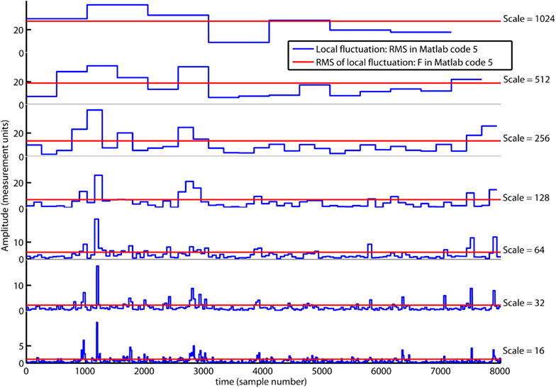
Figure 4. The local fluctuations, RMS{ns} (blue lines), computed by Matlab code 5 for segments with multiple segment sizes (i.e., scale). The scaling function F{ns} is the overall RMS (red line) of the local fluctuation RMS{ns}. Notice that F{ns} decreases on smaller scales.
DFA indentifies the monofractal structure of a time series as the power law relation between the overall RMS (i.e., F in Matlab code 4) computed for multiple scales (i.e., scale in Matlab code 5). The power law relation between the overall RMS is indicated by the slope (H) of the regression line (RegLine) computed by Matlab code 6 below:
Matlab code 6: Part 2 of DFA
C=polyfit(log2(scale),log2(F),1);

H=C(1);

RegLine=polyval(C,log2(scale));
Type plot5 in Matlab command window to access Figure 5.
The slope, H, of the regression line, RegLine, is called the Hurst exponent (Hurst, 1951). The Hurst exponent defines the monofractal structure of the time series by how fast the overall RMS, F, of local fluctuations, RMS, grows with increasing segment sample size (i.e., scale). Figure 5 shows that the overall RMS, F, of local fluctuations, RMS, is growing faster with the segment sample size for the monofractal and multifractal time series compared with whitenoise time series. The larger Hurst exponent, H, is visually seen as more slow evolving variations (i.e., more persistent structure) in monfractal and multifractal time series compared with whitenoise. Figure 6 illustrates that the Hurst exponents defines a continuum between a noise like time series and a random walk like time series. The Hurst exponent will be in the interval between 0 and 1 for noise like time series whereas above 1 for a random walk like time series. A time series has a long-range dependent (i.e., correlated) structure when the Hurst exponent is in the interval 0.5–1 and an anti-correlated structure when the Hurst exponent is in the interval 0–0.5. The time series has an independent or short-range dependent structure in the special case when the Hurst exponent is equal to 0.5. According to Figure 5, time series whitenoise has a time independent structure with Hurst exponent close to 0.5 whereas monofractal, and multifractal has a long-range dependent structure with Hurst exponent between 0.7 and 0.8. The reader should notice that short-range dependent processes can mimic the scale invariance in Figure 5 for certain scaling ranges (cf. Gao et al., 2006).
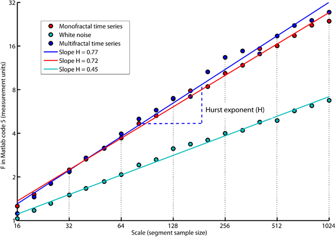
Figure 5. The plot of overall RMS (i.e., F in Matlab code 5) versus the segment sample size (i.e., scale in Matlab code 5) where both F and scale are represented in log-coordinates. The scale invariant relation is indicated by the slope, H, of the regression lines, RegLine, computed by Matlab code 6. The slope, H, is a power law exponent called the Hurst exponent because F and scale are represented in log-coordinates. Notice that both the monofractal and multifractal time series have more apparent slow fluctuations compared to whitenoise indicated by larger amplitudes of the overall RMS on the larger scales.
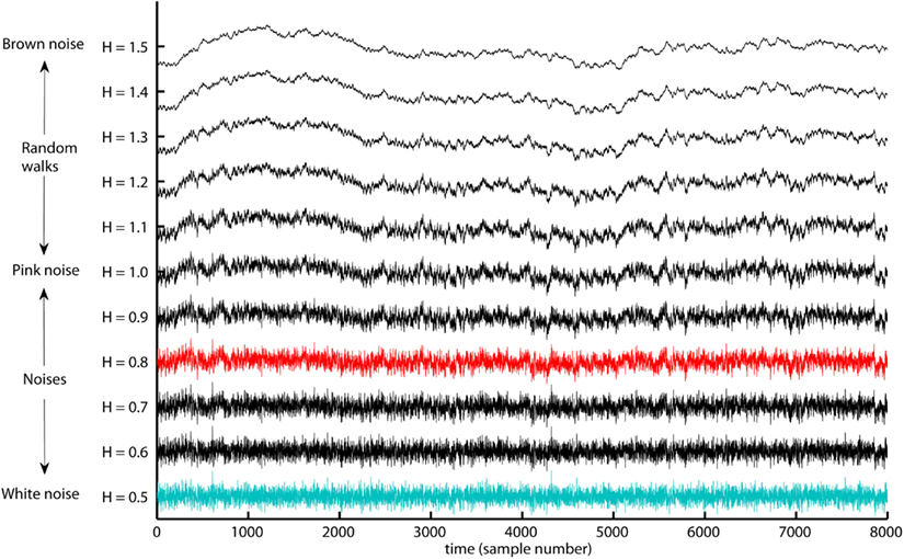
Figure 6. The range of Hurst exponents defines a continuum of fractal structures between white noise (H = 0.5) and Brown noise (H = 1.5). The pink noise H = 1 separates between the noises H < 1 that have more apparent fast evolving fluctuations and random walks H > 1 that have more apparent slow evolving fluctuations. The examples monofractal (red trace) and whitenoise (turquoise trace) used in the present tutorial are both noise like time series. The long-range dependent structure of most biomedical signals is located within the illustrated continuum of fractal structures.
The structure of the monofractal and multifractal time series are different even though they have similar overall RMS and slopes H in Figure 5. The multifractal time series have local fluctuations with both extreme small and large magnitudes that is absent in the monofractal time series. The absence of fluctuations with extreme large and small magnitudes results in a normal distribution for the monofractal time series where the variation is described by the second order statistical moment (i.e., variance) alone. The monofractal DFA are therefore based on the second order statistics of the overall RMS (i.e., F in Matlab code 4). In the multifractal time series, local fluctuation, RMS{ns}(v), will be extreme large magnitude for segments v within the time periods of large fluctuations and extreme small magnitude for segments v within the time periods of small fluctuations. Consequently, the multifractal time series are not normal distributed and all q-order statistical moments should to be considered. Thus, it’s necessary to extend the overall RMS in the monofractal DFA (i.e., F in Matlab code 4) to the following q-order RMS of the multifractal DFA (Fq in Matlab code 7 below):
Matlab code 7:
q=[-5,-3,-1,0,1,3,5];

for nq=1:length(q),

 qRMS{1}=RMS{1}.^q(nq);

 Fq(nq)=mean(qRMS{1}).^(1/q(nq));

end

Fq(q==0)=exp(0.5*mean(log(RMS{1}.^2)));
Type plot7 in the Matlab command window to access Figure 7.
The first command line in Matlab code 7 defines a set of q-orders from −5 to 5. The second line initiates a loop that computes the overall q-order RMS, Fq(nq), from negative to positive q’s (see the red arguments nq). The q-order weights the influence of segments with large and small fluctuations, RMS{1}, as illustrated in Figure 7. Fq(nq) for negative q’s (i.e., nq = 1–3) are influenced by segments v with small RMS{1}(v). In contrast, Fq(nq) for positive q’s (i.e., nq = 4–6) are influenced by segments v with large RMS{1}(v). The local fluctuations RMS{1} with large and small magnitudes is graded by the magnitude of the negative or positive q-order, respectively. Fq for q = −3 and 3 is more influenced by the segments v with the smallest and largest RMS{1}(v), respectively, compared to Fq for q = -1 and 1 (see Figure 7). The midpoint q = 0 are neutral to influence of segments with small and large RMS{1}. Notice that the last line of Matlab code 7 redefines the special case q(nq) = 0 because 1/0 goes to infinity [i.e., 1/q(q = = 0) = inf in Matlab]. The reader should also notice that Fq(q = = 2) are equal to second order statistics F in Matlab code 4 because sqrt(x) = x^(1/2) in Matlab. The monofractal DFA in Matlab code 5 can now be extended to a MFDFA by simply changing Matlab code 4 to Matlab code 7 in the last line of Matlab code 5. This change is highlighted with red command lines in Matlab code 8 below:
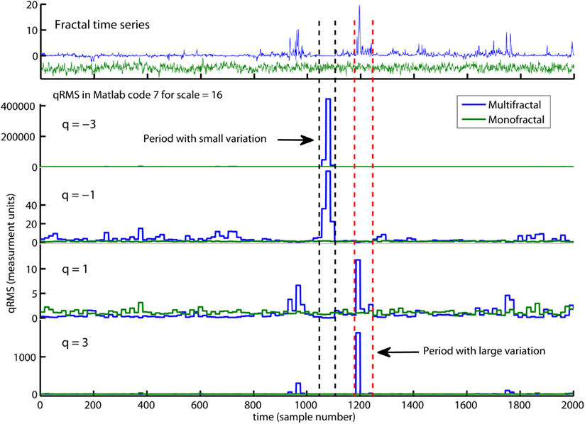
Figure 7. An illustration of qRMS{1} computed by Matlab code 7. qRMS{1} is the q-order of the local fluctuateons (i.e., RMS{1}) and are the building block of the overall q-order RMS (i.e., Fq in Matlab code 7). qRMS{1} is represented for the monofractal (green traces) and multifractal (blue traces) time series. The negative q-order (q = −3 and −1) amplifies the segments in the multifractal time series with extreme small RMS{1} whereas positive q-order (q = 3 and 1) amplifies the segments with extreme large RMS{1}. Notice that q = −3 and q = 3 amplify the small and large variation, respectively, more than q = −1 and q = 1. Notice also that the monofractal time series has no segments with extreme large or small fluctuations and, thus, no peaks in qRMS{1}. The overall q-order RMS is able to distinguish between the structure of small and large fluctuations and, consequently, between the monofractal and multifractal time series.
Matlab code 8 Part 1 of MFDFA1
X=cumsum(multifractal-mean(multifractal));

X=transpose(X);

scale=[16,32,64,128,256,512,1024];

q=[-5,-3,-1,0,1,3,5];

m=1;

for ns=1:length(scale),

 segments(ns)=floor(length(X)/scale(ns));

 for v=1:segments(ns),

  Index=((((v-1)*scale(ns))+1):(v*scale(ns)));

  C=polyfit(Index,X(Index),m);

  fit=polyval(C,Index);

  RMS{ns}(v)=sqrt(mean((X(Index)-fit).^2));

 end

 for nq=1:length(q),

  qRMS{nq,ns}=RMS{ns}.^q(nq);

  Fq(nq,ns)=mean(qRMS{nq,ns}).^(1/q(nq));

 end

 Fq(q==0,ns)=exp(0.5*mean(log(RMS{ns}.^2)));

end
The relationship between Matlab code 8 and the mathematical equations used to introduce the MFDFA in Kantelhardt et al. (2002) are given below:
Eq. 1 in Kantelhardt et al. (2002):
X:
multifractal: x
mean(multifractal): 〈x〉
The number Ns of non-overlapping segments:
segments(ns): Ns ≡ int(N/s)
length(X): N
scale(ns): s
Eq. 4 in Kantelhardt et al. (2002):
RMS{ns}(v): F(s,v)
mean((X(Index)-fit).^2):
Index: (v - 1)s + i for i = 1, 2, …, s
fit:
C: Ck
Eq. 4 in Kantelhardt et al. (2002):
Fq(nq,ns):
qRMS{nq,ns}: [F2(s, v)]q/2
mean(qRMS{nq,ns}):
The q-order Hurst exponent can now be defined as the slopes (Hq) of regression lines (qRegLine) for each q-order RMS (Fq). Both Hq(nq) and qRegLine{nq} is computed by looping Matlab code 6 for each q-order (see red command lines and arguments nq in Matlab code 9 below):
Matlab code 9 Part 2 of MFDFA1
for nq=1:length(q),

 C=polyfit(log2(scale),log2(Fq(nq,:)),1);

 Hq(nq)=C(1);

 qRegLine{nq}=polyval(C,log2(scale));

end
Type plot8 in Matlab command window to access Figure 8.
The relationship between Matlab code 9 are given below in the mathematical notation used in Kantelhardt et al. (2002):
Hq(nq):       h(q)

qRegLine{nq}:    log2(Fq (s)) = h(q) log2 (s) + C
Figure 8 shows that the slopes Hq of the regression lines are q-dependent for the multifractal time series (see Figure 8A). The difference between the q-order RMS for positive and negative q’s are more visual apparent at the small segment sizes compared to the large segment sizes (see Figure 8A). The small segments are able to distinguish between the local periods with large and small fluctuations (i.e., positive and negative q’s, respectively) because the small segments are embedded within these periods. In contrast, the large segments cross several local periods with both small and large fluctuations and will therefore average out their differences in magnitude. Thus, the relationship between the q-order RMS of the multifractal time series becomes similar to the monofractal time series at the largest segment sizes (compare Figures 8A,B). Both the monofractal and whitenoise time series have no periods with small and large fluctuations and, consequently, the same difference between the q-order RMS irrespective of the segment sample sizes (see Figures 8B,C). The growing similarity between the q-order RMS of multifractal and monofractal time series with increasing segment sample size leads to a decreasing Hq for multifractal time series (see Figure 8D). The decreasing Hq indicates that the segments with small fluctuations have a random walk like structure whereas segments with large fluctuations have a noise like structure (see the continuum of Hurst exponents in Figure 6). The similarity between the scaling function F of monofractal and multifractal time series in Figure 5 is indicated by the intercept of Hq around q = 2 (compare blue and red traces in Figure 8D). Thus, the monofractal DFA in Matlab code 5 and 6 will not distinguish between the structure of the monofractal and multifractal time series.
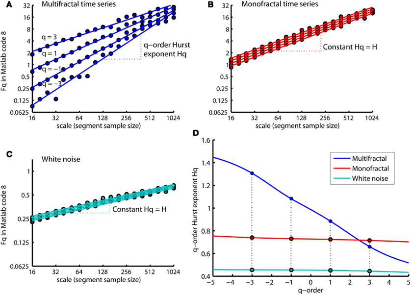
Figure 8.
q-order RMS Fq(nq,:) and corresponding regression line qRegLine{nq} computed by MFDFA (i.e., Matlab code 8 and 9) for time series multifractal (A), monofractal (B), and whitenoise (C). (A) The scaling functions Fq (blue dots) and corresponding regression slopes Hq (blue dashed lines) are q-dependent. (B,C) The scaling functions Fq (red and turqouish dots) and regression slope Hq (red and turqouish dashed lines) are q-independent. (D) The q-order Hurst exponent Hq for the time series multifractal (blue trace), monofractal (red trace) and whitenoise (turqouish trace) where the colored dots represents the slopes Hq for q = −3, −1, 1, and 3 illustrated in (A–C). Notice that the intercept of Hq for multifractal and monofractal time series [intercept between blue and red trace in (D)] are close to q = 2. This intercept reflects the similarity between their overall RMS, F, in Figure 5.
The q-order Hurst exponent Hq is only one of several types of scaling exponents used to parameterize the multifractal structure of time series. The typical procedure in the literature of MFDFA is to first convert Hq to the q-order mass exponent (tq) and thereafter convert tq to the q-order singularity exponent (hq) and q-order singularity dimension (Dq; Kantelhardt et al., 2002). The plot of hq versus Dq is referred to as the multifractal spectrum (see Figure 9C). The q-order mass exponent tq can be computed from Hq by the Matlab code 10 below (see Figure 9B):
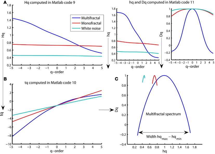
Figure 9. Multiple representations of multifractal spectrum for multifractal (blue traces), monofractal (red traces), and whitenoise (turquoise trace) time series. (A) q-order Hurst exponent Hq computed in Matlab code 9. (B) Mass exponent tq computed in Matlab code 10. (C) Multifractal spectrum of Dq and hq (upper right panels) computed in Matlab code 11 and plotted against each other. The arrow indicates the difference between the maximum and minimum hq that are called the multifractal spectrum width. Notice that the constant Hq for monofractal and whitenoise times series leads to a linear tq that further leads to a constant hq and Dq that, finally, are joined to become only tiny arcs in (C).
Matlab code 10 Part 3 of MFDFA1
tq=Hq.*q-1;
Eq. 13 in Kantelhardt et al. (2002)
The mass exponent tq is used to compute the q-order singularity exponent (hq) and the q-order singularity dimension (Dq) by Matlab code 11 below (see upper right Figure 9):
Matlab code 11 Part 4 of MFDFA1
hq=diff(tq)./(q(2)-q(1));

Dq=(q(1:end-1).*hq)-tq(1:end-1);
Equation 15 in Kantelhardt et al. (2002)
Type plot9 in the Matlab command window to access Figure 9.
The monofractal and whitenoise time series has a mass exponent tq with a linear q-dependency. The linear q-dependency of tq leads to a constant hq of these time series because hq is the tangent slope of tq (see the first command line in Matlab code 11). The constant hq reduces the multifractal spectrum to a small arc for the monofractal and whitenoise time series (see Figure 9C). In contrast, the multifractal time series has mass exponents tq with a curved q-dependency and, consequently, a decreasing singularity exponent hq. The resulting multifractal spectrum is a large arc where the difference between the maximum and minimum hq are called the multifractal spectrum width (see arrow in Figure 9C).
The reader should notice that the q-order singularity exponent hq and corresponding dimension Dq computed by Matlab code 11 are referred to as α and f(α) in Kantelhardt et al. (2002), but as h and D(h) in other literature (e.g. Ihlen and Vereijken, 2010). Furthermore, the singularity dimension can be confused with the generalized dimension and the box counting dimension that is other ways to parameterize the multifractal structure of time series (see Equation 14 in Kantelhardt et al., 2002).
The Hurst exponent defined by the monofractal DFA represents the average fractal structure of the time series as illustrated in Figure 6 and is closely related to the central tendency of multifractal spectrum. The deviation from average fractal structure for segments with large and small fluctuations is represented by the multifractal spectrum width. Thus, each average fractal structure in the continuum of Hurst exponents (see Figure 6) has a new continuum of multifractal spectrum widths that represents the deviations from the average fractal structure (see Figure 10). Furthermore, the shape of the multifractal spectrum in Figure 10 does not have to be symmetric. The multifractal spectrum can also have either a left or a right truncation that originate from a leveling of the q-order Hurst exponent for negative or positive q’s, respectively (see Figure 11). The leveling of q-order Hurst exponent reflects that the q-order RMS is insensitive to the magnitude of the local fluctuations. The multifractal spectrum will have a long left tail when the time series have a multifractal structure that is insensitive to the local fluctuations with small magnitudes (see upper Figure 11). In contrast, the multifractal spectrum will have a long right tail when the time series have a multifractal structure that is insensitive to the local fluctuations with large magnitudes (see lower Figure 11). Another continuum of right and left truncations exists for each multifractal spectrum width in the continuum illustrated in Figure 10. Thus, the width and shape of the multifractal spectrum is able to classify a wide range of different scale invariant structures of biomedical time series.
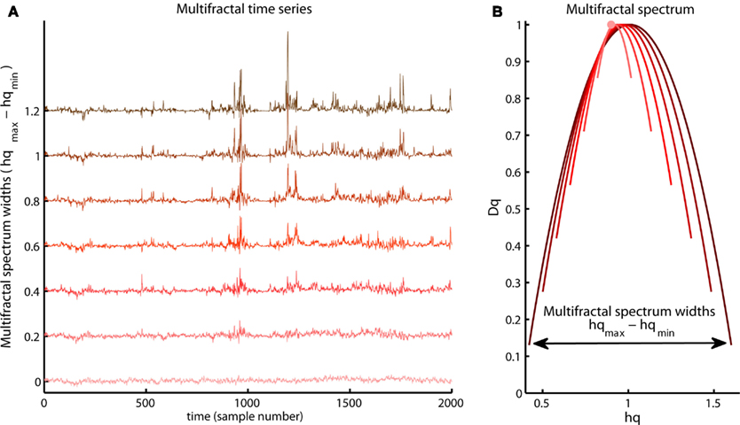
Figure 10. Illustration of a continuum of multifractal time series with the same q-order Hurst exponent for q = 2 but with different multifractal spectrum width [compare vertical axis of the (A) and the arrow in the (B)]. Notice the growth of structural differences between the periods with small and large fluctuations as the multifractal spectrum width become larger.
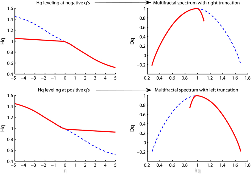
Figure 11. Illustration of multifractal spectra with a right truncation (upper right panel) and a left truncation (upper left panel). These truncations originate from the leveling of the q-order Hurst exponents for negative q’s (upper right panel) and positive q’s (upper left panel), respectively.
The transformation of the q-order Hurst exponent Hq to the mass exponent tq and, finally, to the multifractal spectrum Dq and hq is stated as a “just-the-way-it-is” argument in the above section without mathematical details. The reader might ask at this point why one should define and interpret the multifractal spectrum Dq and hq and not only Hq that are directly estimated by Matlab code 8 and 9. Estimating the multifractal spectrum directly from the local fluctuation, will answer this question and give a less abstract definition of the multifractal spectrum. A local Hurst exponent can be defined directly from, RMS{ns}(v), for each time instant v. The local Hurst exponent estimated for a multifractal time series will fluctuate in time in contrast to the time independent Hurst exponent estimated by the monofractal DFA (see Matlab code 5 and 6; Figure 5). The temporal variation of the local Hurst exponent can be summarized in a probability distribution and the multifractal spectrum is just the normalized probability distribution in log-coordinates. Thus, the width and shape of the multifractal spectrum reflect the temporal variation of the local Hurst exponent or, in other words, the temporal variation in the local scale invariant structure of the time series. In order to estimate the local Hurst exponent, the local fluctuation, RMS{ns}(v), has to be defined within a translating segment centered at sample v instead of within non-overlapping segments. Thus, Matlab code 8 has to be modified to Matlab code 12 below (see red command lines):
Matlab code 12 Part 1 of MFDFA2
X=cumsum(multifractal-mean(multifractal));

X=transpose(X);

scale_small=[7, 9, 11, 13, 15, 17];

halfmax=floor(max(scale_small)/2);

Time_index=halfmax+1:length(X)-halfmax;

m=1;

for ns=1:length(scale_small),

 halfseg=floor(scale_small(ns)/2);

 for v=halfmax+1:length(X)-halfmax;

  T_index=v-halfseg:v+halfseg;

  C=polyfit(T_index,X(T_index),m);

  fit=polyval(C,T_index);

  RMS{ns}(v)=sqrt(mean((X(T_index)-fit).^2));

 end

end
(The reader must be patient because this code might take a couple of minutes)
The first red command line defines a vector of small segment sizes (i.e., scale_small) where the segment sizes increases with two samples. This increase of two samples is necessary to align the center of segments according to the Time_index. The third red line set the Time_index for the local fluctuation, RMS{ns}, that exclude the halfmax number of samples at the start and the end of the time series (see second red command line). Then a loop are initiated for each segment size where the local fluctuations, RMS{ns}(v), are computed for a translating segment centered at sample v = Time_index. The translating segment includes the local samples that are updated by T_index (see last red command line). The local Hurst exponent (Ht) can now be computed from the local fluctuation, RMS{ns}, by the Matlab code 13 below:
Matlab code 13 Part 2 of MFDFA2
C=polyfit(log2(scale),log2(Fq(q==0,:)),1);

Regfit=polyval(C,log2(scale_small));

maxL=length(X);

for ns=1:length(scale_small);

  RMSt=RMS{ns}(Time_index);

  resRMS{ns}=Regfit(ns)-log2(RMSt);

  logscale(ns)=log2(maxL)-log2(scale_small(ns));

  Ht(ns,:)=resRMS{ns}./logscale(ns)+Hq(q==0);

end
Type plot12 in the Matlab command window to access Figure 12.
The first two command line defines the regression line Regfit equal to the regression line qRegLine{q }= computed by Matlab code 8. = 0
Regfit represents the center of the spread of local RMS and are the regression line of the overall q-order RMS, Fq(q = = 0,:). A loop for each scale ns computes the residual fluctuation resRMS{ns} of log2(RMS{ns}) around the regression line Regfit for each sample v of the time series. In Figure 12B, the differences between the overall q-order RMS, Fq, converge toward each other with increasing scale. This convergence is inevitable for multifractal variation by the linear relationship between Fq for all q-order and the assumption of monotonical decreasing q-order Hurst exponent, Hq (see Figure 8D). The same convergence is seen for the local RMS in Figure 12A and is used to estimate the local Hurst exponents, Ht(ns,:). Ht(ns,:) is estimated as the slope of the line from local RMS in log-coordinates to the endpoint of the regression line, Regfit, at the largest scale, maxL (see Figure 12). Consequently, Ht(ns,:) are obtained by dividing the residuals resRMS{ns} by logscale (i.e., the difference between maximal scale maxL and the scale(ns) in log-coordinates) and adding the slope Hq(q = = 0) of regression line, Regfit (see Figure 12A). Figure 13A illustrates the local Hurst exponent Ht(ns,:) for ns = 5 (i.e., scale(ns) = 15) for the multifractal, monofractal, and whitenoise time series. The local Hurst exponent Ht(ns,:) has larger variation for the multifractal time series compared to the monofractal and whitenoise time series. The small Ht(ns,:) in the periods of the multifractal time series with local fluctuations of large magnitudes (i.e., large RMS{ns}) reflects the noise like structure of the local fluctuations (see red dashed lines in Figure 13A). In contrast, the larger Ht(ns,:) in the periods with local fluctuations of small magnitudes (i.e., small RMS{ns}) reflects the random walk like structure of the local fluctuations (see black dashed lines in Figure 13A). The local Hurst exponent Ht in periods with fluctuations of small and large magnitudes is therefore consistent with the q-order Hurst exponent Hq for negative and positive q’s, respectively. The advantage of local Hurst exponent Ht compared with q-order Hurst exponent Hq is the ability of Ht to identify the time instant of structural changes within the time series. In studies where the physiological phenomenon is perturbed at some time instant v, the local Hurst exponent Ht(ns,v) can identify how this perturbation affects the local scale invariant structure of the biomedical time series. The temporal variation of local Hurst exponent Ht can be summarized in a histogram representing the probability distribution (Ph) of Ht (see Figure 13B). The multifractal spectrum (Dh) is defined simply by the log-transformation of the normalized probability distribution (Ph_norm). The probability distribution (Ph) and multifractal spectrum (Dh) are computed by Matlab code 14 below:
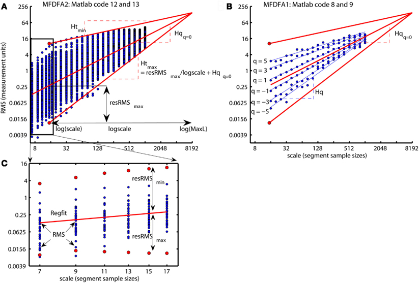
Figure 12. (A) A summary of how the local Hurst exponent Ht is estimated in Matlab code 13. The regression line Regfit (red center line) is the center of the spread of local RMS in log-coordinates and is equal to the regression line qRegLine{q }= in Matlab code 8 and 9 [see (B)]. The minimum and maximum local Hurst exponent = 0
Ht(5,:) is the slope of the upper and lower red lines, respectively, that converge from the maximum and minimum of RMS{5} onto the regression line Regfit at the maximum scale maxL. Consequently, the local Hurst exponent Ht(ns,:) estimated by dividing the residual resRMS{ns}(v) for each time instant v by logscale(ns) (i.e., the difference between the maximal scale maxL and scale(ns) in log-coordinates) and adding the slope Hqq=0 of the regression line Regfit. (B) The scaling function Fq (blue dots) and the regression lines qRegLine{nq} (blue lines) computed by Matlab code 8 and 9. All Fq lies within the envelope between the red lines for the maximum and minimum Ht(5,:), but does not cover the entire range in the same way as the local RMS{5} in (A). (C) The smallest scales used to compute the local Hurst exponents and the multifractal spectrum illustrated in Figure 13. The red dots represent the maximum RMS{ns}(1080) and minimum RMS{ns}(1199) for multiple segment sample sizes [i.e., scale(ns)] at time instant v = 1080 and v=1199, respectively [see Figure 13A] whereas blue dots represent the local fluctuations for 30 other time instants. Notice that both the horizontal and vertical axes in all panels are in log-coordinates.
Matlab code 14 Part 3 of MFDFA2
Ht_row=Ht(:);

BinNumb=round(sqrt(length(Ht_row)));

[freq,Htbin]=hist(Ht_row,BinNumb);

Ph=freq./sum(freq);

Ph_norm=Ph./max(Ph);

Dh=1-(log(Ph_norm)./-log(mean(scale)));
Type plot13 in Matlab command window to access Figure 13.
The first line in Matlab code 14 convert the matrix Ht to the vector Ht_row that are the input argument in hist function used to compute the histogram for Ht_row. The second input argument in hist function are BinNumb that set the number of bins in the histogram. A sufficient choice for BinNumb is the square root of the sample size of Ht_row (see the second command line). The output variables of hist function are the center of each bin Htbin and the number freq of local Hurst exponents that fall into each bin. The probability distribution Ph are computed by dividing the number freq of local Hurst exponents in each bin by the total number of local Hurst exponents, sum(freq) (see Figure 13B). The multifractal spectrum Dh are computed by first define Ph_norm by normalizing Ph to the maximum probability max(Ph) and then divide log(Ph_norm) by –log(mean(scale)) (cf. Struzik, 2000; Scafetta et al., 2003). The multifractal spectrum Dh are therefore directly related to the distribution Ph of the local fractal structure of the time series. The distribution Ph is the same for the local scale invariant structure of the time series as the conventional probability distribution are for the local amplitudes of the time series. The present state of the physiological system is connected to both past and future states that influence the local scale invariant structure of time series. Thus, distribution Ph and the multifractal spectrum Dh of biomedical time series might reflect important properties of the self-regulation of physiological processes.
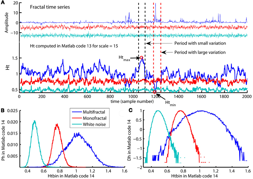
Figure 13. (A) The multifractal, monofractal, and whitenoise time series (upper panel) and their local Hurst exponents Ht(:,5) computed by Matlab code 13 (lower panel). The multifractal time series have a larger variation in the local Hurst exponents Ht(5,:) compared with the monofractal and whitenoise time series. The period with the local fluctuation of the smallest magnitude in multifractal time series contains the maximum Ht(5,:) (see Htmax in period between the black dashed lines) whereas the period with the local fluctuation of the largest magnitudes contains the smallest Ht(5,:) (see Htmin in the period between red dashed lines). (B) The probability distribution Ph of the local Hurst exponents Ht estimated as histograms by Matlab code 14 for the multifractal, monofractal, and whitenoise time series. (C) The multifractal spectrum Dh estimated from distribution Ph by Matlab code 14 for the same time series. The distribution Ph and spectrum Dh have a larger width for the multifractal time series compared to the monofractal and whitenoise time series.
The MFDFA introduced piece-by-piece in Section “Multifractal Detrended Fluctuation Analysis in Matlab” can be combined into two Matlab function MFDFA1 and MFDFA2, respectively:
Matlab functions for MFDFA
Matlab code 8 to 11:
[Hq,tq,hq,Dq,Fq]=MFDFA1(signal,scale,q,m,Fig);
Matlab code 12 to 14:
[Ht,Htbin,Ph,Dh]=MFDFA2(signal,scale,m,Fig);
Type help MDFA1 or help MFDFA2 in the Matlab command window to access the definition of the input and output variables. The help functions provide examples for the employment of MFDFA1 and MFDFA2 to time series.
The main aim of Section “The Best Practice of Multifractal Detrended Fluctuation Analysis” is to guide the application of MFDFA1 and MFDFA2 to biomedical time series. In Section “Multifractal Detrended Fluctuation Analysis in Matlab” the readers has gained insight into the construction of MFDFA1 and MFDFA2 and this insight will help them to avoid potential pitfalls in the application of MFDFA1 and MFDFA2. The best practice of MFDFA1 and MFDFA2 has several steps. First, the structure of biomedical time series must be similar to noise before employing MFDFA1 and MFDFA2 (see blue traces in Figure 1). Section “Random Walk or Noise Like Time Series?” introduces conversions to make the biomedical time series similar to a noise like time series. Secondly, the local fluctuations within the biomedical time series cannot be close to zero. Section “Local Fluctuations Close to Zero?” discusses possible origins for local fluctuations close to zero and possible solutions to this problem. Thirdly, the biomedical time series must be scale invariant within the predefined range of scales. Section “Is the Time Series Scale Invariant?”3 discusses the general assumption of a scale invariant time series as input in MFDFA1 and MFDFA2. Fourth, the input parameters scale, q, and m in MFDFA1 and MFDFA2 must be sufficiently defined for each biomedical time series. Section “How to Set the Input Parameters Scale, q, and m in MFDFA1 and MFDFA2” introduces guidelines for the optimal parameter setting. Finally, Section “Other Multifractal Analysis” lists other multifractal analyses where results can be compared to results from MFDFA1 and MFDFA2.
MFDFA1 and MFDFA2 have the best performance when signal are a noise like time series. However, it can be difficult according to Figure 6 to visually differentiate between random walk and noise like time series. A possible solution suggested by Eke et al. (2002) is to run a monofractal DFA (i.e., Matlab code 5 and 6) before running MFDFA1 and MFDFA2. The time series are noise like if Hurst exponent H is between 0.2 and 0.8. In this case, MFDFA1 and MFDFA2 can be employed directly without transformation of the time series. However, the time series are random walk like when H is between 1.2 and 1.8. In these cases, the time series should either be differentiated before entering the MFDFA1 or MFDFA2 or the conversion to random walk in the first line of Matlab code 8 and 12 should be eliminated. If the time series are random walk like + 1 should be added to the output variables Hq, hq, and tq from MFDFA1 and Ht and Htbin from MFDFA2. Table 1 summarize the categories of the Hurst exponent estimated by a monofractal DFA with corresponding conversion of the biomedical time series that should be performed before entering it into MFDFA1 and MFDFA2.
The local fluctuation in the time series is defined as a local RMS within both MFDFA1 and MFDFA2. Large error appears in the multifractal spectrum when RMS is close to zero because both log2(Fq) for negative q’s in Matlab code 8 and log2(RMSt) in Matlab code 12 becomes infinitely small (i.e., -inf in Matlab). Extreme large Hq will be present for negative q’s as output from MFDFA1. Equivalently, extreme large outliers in Ht will be present as output from MFDFA2. Consequently, local RMS close to zero will lead to large right tails for the multifractal spectrum. The problem of segments with RMS close to zero can be solved by eliminating RMS below a certain threshold (eps). The threshold eps can be set to the precision of the measurement device that is recording the biomedical time series. As an example, the measurement of the inter-beat intervals of the human heart is measured as the time interval between R-peaks in ECG and has a typical precision of 1 millisecond. Thus, RMS below 1 millisecond can be eliminated from further analysis when MFDFA1 and MFDFA2 are employed to series of inter-beat intervals. Elimination of local fluctuations below the measurement error is possible in MFDFA1 by setting eps = 1 and RMS{ns}(RMS < eps) = [] in Matlab code 8.
There are two main reasons why the local fluctuation RMS becomes zero in segments with small sample sizes. First, the polynomial trend fit of the time series can be overfitted in segments with small sample sizes (i.e., small scale). An overfitted trend will be similar to the time series and cause the residual fluctuations, RMS, to be close to zero. The sample size of the smallest segment (i.e., scale) should therefore be much larger than the polynomial order m to prevent an overfitted trend. Secondly, the biomedical time series might be smooth with little apparent variation and therefore similar to the polynomial trend even for low order m. In these cases, the value of the smallest scales should be raised and the scale invariance checked carefully (see “Is the Time Series Scale Invariant?” below).
The application of both Matlab function MFDFA1 and MFDFA2 assumes that the biomedical time series are scale invariant. This means that plot(log2(scale),log2(Fq)) yield a linear relationship between log2(scale) and log2(Fq) (see Figure 8)., The q-order Hurst exponent Hq should not be estimated by a linear regression if the relationship between log2(scale) and log2(Fq) is curved or S-shaped. Consequently, the first output from MFDFA1 to be visually checked should be plot(log2(scale),log2(Fq)). Non-linear relation in this plot might arise from several reasons. First, an insufficient order m for the polynomial detrending will yield a non-linear relationship between log2(scale) and log2(Fq) for scale invariant time series with a trend. The solution is to run MFDFA1 or MFDFA2 multiple times with different m and compare their plot(log2(scale),log2(Fq). Secondly, local fluctuations RMS close to zero for small scales would yield a non-linear dip in lower end of plot(log2(scale),log2(Fq)). This dip can be prevented by elimination of RMS below the measurement error suggested in Section “Local Fluctuations Close to Zero?” or by choosing a larger minimum input scale. Finally and most importantly, a non-linear relationship in plot(log2(scale),log2(Fq)) might originate from the phenomenon recorded in the biomedical time series. As an example, respiratory frequency creates distinct oscillations in the fast fluctuations of the heart rate variability (Stein and Kleiger, 1999) and cause the scale invariance to break down at the smallest scales. Another example is postural sway in humans where the variation of the center of pressure has two distinct scaling regions thought to represent two distinct modes for human balance control (Collins and De Luca, 1993). One way to detect the sub-regions with scale invariance is to look for periods with approximately constant log2(Fq(q = = 1,:)./scale) in plot(log2(scale),log2(Fq(q = = 1,:)./scale)) within the entire scaling range (cf. Gao et al., 2006). The scales where log2(Fq(q = = 1,:)./scale) are no longer constant indicates the segment sizes above and below which the local fluctuations (i.e., RMS) are no longer scale invariant. These points will in many cases have phenomenological explanations and should not be ignored.
The Matlab functions MFDFA1 and MFDFA2 have input parameters scale, q and m. The estimation of the multifractal spectra is dependent on these parameter settings. The rest of this section gives guidelines to the parameter settings in MFDFA1 and MFDFA2:
The input parameters scale is the multiple segment sizes for the computation of local fluctuation RMS in Matlab code 8 and 12. A minimum and maximum sample size of the segments [i.e., min(scale) and max(scale) in Matlab] has to be chosen to construct the set of scales used in MFDFA1 and MFDFA2. Both statistical and phenomenological arguments exist on how to choose the minimum and maximum segment size. The statistical argument is to choose minimum and maximum segment sizes that provide a numerical stable estimation of RMS and Fq in Matlab code 8 and 12. The minimum segment sample size should be large enough to prevent error in the computation of local fluctuation RMS. The minimum segment size larger than 10 samples is a “rule of tumb” for the computation of RMS. Furthermore, the minimum sample size must be considerably larger than the polynomial order m to prevent overfitting of polynomial trend (see “Local Fluctuations Close to Zero?” above). Thus, minimum segment size of 10 samples might be too small for large trend order m (Kantelhardt et al., 2002). In MFDFA1, the maximum segment size should be small enough to provide a sufficient number of segments in the computation of Fq in Matlab code 8. A maximum segment size below 1/10 of the sample size of the time series will provide at least 10 segments in the computation of Fq in Matlab code 8. Furthermore, it’s favorable to have a equal spacing between scales when they are represented in plot(log2(scale),log2(Fq)) to obtain a optimal performance of the linear regression that estimates q-order Hurst exponent Hq. Equal spacing between log2(scale) is provided by Matlab code 15 below:
Matlab code 15:
scmin=16;
scmax=1024;
scres=19;
exponents=linspace(log2(scmin),log2(scmax),scres);
scale=round(2.^exponents);
Matlab code 15 is employed before running MFDFA1 where the minimum segment size, scmin, maximum segment size, scmax, and the total number of segment sizes, scres, are predefined. The segment sizes (i.e., scale) in MFDFA2 should be small in order to provide a stable estimation of the probability distribution Ph and, consequently, the multifractal spectrum Dh (Scafetta et al., 2003). The local Hurst exponent Ht for large scale will have a smooth and slow varying dynamics that are not well described by a probability distribution Ph. Thus, a small scaling range like scale= [7,9,11,13,15,17] used in Matlab code 12 are preferable in MFDFA2. However, the reader should notice that the small segment sizes (i.e., scale) in MFDFA2 come at the expense of a less precise estimation of the local fluctuation RMS. The imprecise estimation of RMS can be seen as measurement noise of the local Hurst exponent Ht present for the monofractal and whitenoise time series in Figure 13A. The measurement noise in Ht is represented as a distribution Ph and multifractal spectrum Dh for monofractal and whitenoise time series with a non-zero width (see Figures 13B,C).
Phenomenological argumentations are important for the choice of minimum and maximum segment sizes within the boundaries that provide numerical stable computations. For example, it is unlikely that the movement of the center of mass is faster than 10 Hz during postural sway. If ground reaction force is sampled at 200 Hz by a force plate then the minimum segment size should be larger than 200/10 Hz = 20 samples. Another example is to exclude the smallest segment sizes in heart rate variability known to be dominated by oscillations due to the respiratory frequency. Furthermore, heart rate variability operates with several ranges of scales (i.e., fluctuations with high frequency, low frequency, very low frequency, ultra low frequency) that are suggested to be influenced by different mechanisms (e.g., respiratory frequency, baroceptive responses, circadian rhythm; e.g., Stein and Kleiger, 1999). Three scale invariant sub-bands are also found in EEG signal where the Hurst exponent are able to separate between healthy subjects and epileptic subjects (Gao et al., 2011). Thus, MFDFA1 can be employed to sub-bands of the scaling range in these phenomena (e.g., Makowiec et al., 2011).
The input parameter q in MFDFA1 decides the q-order weighing of the local fluctuation RMS in Matlab code 8. The q-orders should consist of both positive and negative q’s in order to weight the periods with large and small variation in a time series. The precision of the computation of the q-order Hurst exponent Hq decreases with increasing negative and positive q-orders. This imprecision are explained by the result in Figure 7. The single segment with the smallest and largest variation RMS will tower up as a single skyscraper by increasing negative and positive q-orders, respectively, and completely dominate the scaling function Fq (i.e., overall q-order RMS in Matlab code 7). The domination of the single segments with the smallest and largest variation destabilizes Fq and leads to an increasing spread around the regression lines of Fq (see q = 3 and -3 in Figure 8A). The choice of q-orders should therefore avoid large negative and positive values because they inflict larger numerical errors in the tails of the multifractal spectrum. The stability of the computation of the multifractal spectrum is also dependent on the differences between the segments of largest and smallest variation. Time series that have large multifractal spectrum width will have large differences between the segments with the smallest and largest variation and, consequently, destabilize the computation of Fq at smaller negative and positive q-orders (compare multifractal scaling in Figure 8A with the monofractal scaling in Figure 8B). A sufficient choice of q-orders will be between – 5 and 5 for most biomedical time series (Lashermes et al., 2004). The destabilization of the Fq at large negative and positive q-orders is also dependent on the sample size of the time series. Time series with large sample size will have multiple segments with extremely large and small variation whereas time series with moderate sample size will only have a single segment. Multiple segments of large and small variation would stabilize the computation of Fq for large negative and positive q-orders. There exists no consensus for the definition of a “too small” sample sizes for multifractal analyses, but the reader should interpret the result with caution when MFDFA1 and MFDFA2 are employed to time series with less than 1000 samples.
In both MFDFA1 and MFDFA2, the local fluctuation RMS is computed around a polynomial trend where its shape is defined by the order m. A higher order m yield a more complex shape of the trend, but might lead to overfitting for time series within small segment sizes as discussed in Section “Local Fluctuations Close to Zero?” above. Thus, m = 1–3 are probably a sufficient choice when the smallest segment sizes contains 10–20 samples. Most studies that employ DFA to biomedical time series do not report the details of the polynomial detrending. Still, the multifractal spectrum for multiple orders m should be compare to ensure that the multifractal spectrum are not influenced by non-stationary trends in the time series. The trends present in biomedical signals do not have to be of a polynomial shape but might have oscillatory or ramp-like shapes. Both MFDFA1 and MFDFA2 can be extended to include more adaptive detrending procedures like wavelet decomposition (Manimaran et al., 2009), moving average (Carbone et al., 2004), and empirical mode decomposition (Qian et al., 2009). Furthermore, an adaptive fractal analysis is shown to perform better than the DFA with polynomial detrending when employed to biomedical time series with strong trends (Gao et al., 2011). Extensions and modification of the detrending procedure in MFDFA1 and MFDFA2 is preferable if MFDFA are employed to biomedical time series with strong trends. Matlab functions for MFDFA with other detrending procedures are available at www.ntnu.edu/inm/geri/software.
The basic component of both MFDFA1 and MFDFA2 are the local fluctuation, RMS. Statistical parameters other than RMS can be used to define the local fluctuation in a time series. In multifractal analyses based on wavelet transformations, the local fluctuation is defined as the convolution product between the time series and a waveform fitted within local segments of the time series (cf. Daubechies, 1992; Mallat, 1999). The results from analyses called wavelet transformation modulus maxima (Muzy et al., 1991), multifractal analysis with wavelet leaders (Jaffard et al., 2006; Wendt, 2008), and gradient modulus wavelet projection (Turiel et al., 2006) can therefore be directly compared with the results from MFDFA1 and MFDFA2. In an entropy-based estimation of the multifractal spectrum, the local fluctuation is defined as the sum of the time series within the local segment relative to the total sum of the entire time series (Chhabra and Jensen, 1989). This method uses a q-order entropy function instead of a q-order RMS and estimates hq and Dq, directly, as the regression slope of the q-order entropy functions. The MFDFA has been shown to perform as well as or better than these multifractal analyses (Kantelhardt et al., 2002; Oświęcimka et al., 2006; Serrano and Figliola, 2009; Huang et al., 2011). However, extensions of detrending procedure in MFDFA1 and MFDFA2 should be considered when the biomedical time series contains strong oscillatory or ramp-like trends (Hu et al., 2009; Huang et al., 2011).
The multifractal spectrum reflects the variation in the fractal structure of the biomedical time series. The multifractal structure of the inter-beat intervals can identify pathological conditions of the human heart (e.g., Ivanov et al., 1999; Wang et al., 2007). The multifractal structure in neural activity can separate the activity of different brain areas and thereby guide more precise neurosurgery (Zheng et al., 2005). The present tutorial has introduced a multifractal time series analysis called MFDFA (Kantelhardt et al., 2002). MFDFA is simply based on the computation of local RMS for multiple segment sizes as illustrated in Section “Multifractal Detrended Fluctuation Analysis in Matlab.” However, special issues in Section “The Best Practice of Multifractal Detrended Fluctuation Analysis” for the best practice of MFDFA are of paramount importance when MFDFA are employed to biomedical time series. First, a monofractal DFA should be employed to ensure that the biomedical time series has a noise like structure. A conversion according to Table 1 should be made if the time series has not a noise like structure. Secondly, local fluctuation close to zero should be eliminated within MFDFA. Thirdly, the presence of scale invariance should be checked by first running MFDFA1 over a large scaling range [e.g., scmin = 10 and scmax = length(signal)/10 in Matlab] and then plot log2(scale) against log2(Fq). If scale invariance is not present for the entire range, then MFDFA1 can be rerun with modified input parameter scale for scale invariant sub-bands within the original scaling range. MFDFA1 should be employed with a q-orders between -5 and 5 and for multiple trend orders m. MFDFA2 should be employed instead of MFDFA1 when the time instant for structural change in the biomedical time series is of importance or when the biomedical time series contain less than 5000 samples.
The author declares that the research was conducted in the absence of any commercial or financial relationships that could be construed as a potential conflict of interest.
Abbound, S., Berenfeld, O., and Sadeh, D. (1991). Simulation of high-resolution QRS complex using ventricular model with a fractal conduction system. Effects of ischemia on high-requency QRS potentials. Circ. Res. 68, 1751–1760.
Atupelage, C., Nagahashi, H., Yamaguchi, M., Sakamoto, M., and Hashiguchi, A. (2012). Multifractal feature descriptor for histopathology. Anal. Cell. Pathol. (Amst.) 35, 123–126.
Bassingthwaighte, J., Van Beek, J., and King, R. (1990). Fractal branchings: the basis of myocardial flow heterogeneities? Ann. N. Y. Acad. Sci. 591, 392–401.
Carbone, A., Castelli, G., and Stanley, H. E. (2004). Time-dependent Hurst exponent in financial time series. Physica A 344, 267–271.
Chhabra, A., and Jensen, R. V. (1989). Direct determination of the f(α) singularity spectrum. Phys. Rev. Lett. 62, 1327–1330.
Collins, J. J., and De Luca, C. J. (1993). Open-loop and closed-loop control of posture: a random-walk analysis of center-of-pressure trajectories. Exp. Brain Res. 95, 308–318.
Eke, A., Herman, P., Bassingthwaighte, J. B., Raymond, G. M., Percival, D. B., Cannon, M., Balla, I., and Ikényi, C. (2000). Physiological time series: distinguish fractal noises from motions. Eur. J. Physiol. 439, 403–414.
Eke, A., Hermann, P., Kocsis, L., and Kozak, L. R. (2002). Fractal characterization of complexity in temporal physiological signals. Physiol. Meas. 23, R1–R38.
Gao, J. B., Hu, J., and Tung, W.-W. (2011). Facilitating joint Chaos and fractal analysis of biosignals through nonlinear adaptive filtering. PLoS ONE 6, e24331.
Gao, J. B., Hu, J., Tung, W.-W., Cao, Y. H., Sarshar, N., and Roychowdhury, V. P. (2006). Assessment of long range correlation in time series: how to avoid pitfalls. Phys. Rev. E Stat. Nonlin. Soft Matter Phys. 73, 016117.
Goldberger, A. L. (1996). Non-linear dynamics for clinicians: chaos theory, fractals, and complexity at the bedside. Lancet 347, 1312–1314.
Goldberger, A. L., Amaral, L. A., Hausdorff, J. M., Ivanov, P. C., Peng, C. K., and Stanley, H. E. (2002). Fractal dynamics in physiology: alterations with disease and aging. Proc. Natl. Acad. Sci. U.S.A. 99, 2466–2472.
Hausdorff, J. M. (2007). Gait dynamics, fractals and falls: finding meaning in the stride-to-stride fluctuations of human walking. Hum. Mov. Sci. 26, 555–589.
Hu, J., Gao, J. B., and Wang, X. S. (2009). Multifractal analysis of sunspot time series: the effects of the 11-year cycle and Fourier truncation. J. Stat. Mech. P02066, 1–20.
Huang, X. Y., Schmitt, F. G., Hermand, J.-P., Gagne, Y., Lu, Z. M., and Liu, Y. L. (2011). Arbitrary-order Hilbert spectral analysis for time series possessing scaling statistics: a comparison study with detrended fluctuation analysis and wavelet leaders. Phys. Rev. E Stat. Nonlin. Soft Matter Phys. 84, 016208.
Ihlen, E. A. F., and Vereijken, B. (2010). Interaction dominant dynamics in human cognition: beyond 1/fα fluctuations. J. Exp. Psychol. Gen. 139, 436–463.
Ivanov, P. C., Amaral, L. A. N., Goldberger, A. L., Havlin, S., Rosenblum, M. G., Struzik, Z., and Stanley, H. (1999). Multifractality in human heartbeat dynamics. Nature 399, 461–465.
Jaffard, S., Lashermes, B., and Abry, P. (2006). “Wavelet leaders in multifractal analysis,” in Wavelet Analysis and Applications, ed. T. Qian, M. I. Vai, and Y. Xu (Basel: Birkhäuser Verlag), 219–264.
Kantelhardt, J. W., Koscielny-Bunde, E., Rego, H. A. A., Havlin, S., and Bunde, A. (2001). Detecting long-range correlation with detrended fluctuation analysis. Physica A 295, 441–454.
Kantelhardt, J. W., Zschiegner, S. A., Koscielny-Bunde, E., Havlin, S., Bunde, A., and Stanley, H. E. (2002). Multifractal detrended fluctuation analysis of nonstationary time series. Physica A 316, 87–114.
Krenz, G., Linehan, J., and Dawson, C. (1992). A fractal continuum model of the pulmonary arterial tree. J. Appl. Physiol. 72, 2225–2237.
Lashermes, B., Abry, P., and Chainais, P. (2004). New insight in the estimation of scaling exponents. Int. J. Wavelets Multi. 2, 497–523.
Lopes, R., and Betrouni, N. (2009). Fractal and multifractal analysis: a review. Med. Image Anal. 13, 634–649.
Makowiec, D., Rynkiewicz, A., Wdowczyk-Szulc, J., Zarczyńska-Buchowiecka, M., Galaska, R., and Kryszewski, S. (2011). Aging in autonomic control by multifractal studies of cardiac interbeat intervals in the VLF band. Physiol. Meas. 32, 1681–1699.
Manimaran, P., Panigrahi, P. K., and Parikh, J. C. (2009). Multiresolution analysis of fluctuations in non-stationary time series through discrete wavelets. Physica A 388, 2306–2314.
Muzy, J. F., Bacry, E., and Arneodo, A. (1991). Wavelets and multifractal formalism for singular signals: application to turbulence data. Phys. Rev. Lett. 67, 3515–3518.
Oświęcimka, P., Kwapien, J., and Drozdz, S. (2006). Wavelet versus detrended fluctuation analysis of multifractal structures. Phys. Rev. E Stat. Nonlin. Soft Matter Phys. 74, 016103.
Parkinson, I., and Fazzalari, N. (1994). Cancellous bone structure analysis using image analysis. Australas. Phys. Eng. Sci. Med. 470, 64–70.
Peng, C. K., Havelin, S., Stanley, H. E., and Goldberger, A. L. (1995). Quantification of scaling exponents and crossover phenomena in nonstationary time series. Chaos 5, 82–89.
Peng, C. K., Mietus, J. E., Liu, Y., Lee, C., Hausdorff, J. M., Stanley, H. E., Goldberger, A. L., and Lipsitz, L. A. (2002). Quantifying fractal dynamics of human respiration: age and gender effects. Ann. Biomed. Eng. 30, 683–692.
Qian, X.-Y., Zhou, W.-X., and Gu, G.-F. (2009). Modified Detrended Fluctuation Analysis Based on Empirical Mode Decomposition. Available at: http://arxiv.org/PS_cache/arxiv/pdf/0907/0907.3284v1.pdf
Scafetta, N., Griffin, L., and West, B. J. (2003). Hölder exponent spectra for human gait. Physica A 328, 561–583.
Serrano, E., and Figliola, A. (2009). Wavelet leaders: a new method to estimate the multifractal singularity spectra. Physica A 388, 2793–2805.
Stein, P., and Kleiger, E. (1999). Insights from the study of the heart rate variability. Ann. Rev. Med. 50, 249–261.
Struzik, Z. R. (2000). Determining local singularity strengths and their spectra with the wavelet transform. Fractals 8, 163–179.
Suckling, J., Wink, A. M., Bernard, F. A., Barnes, A., and Bullmore, E. (2008). Endogenous multifractal brain dynamics are modulated by age, cholinergic blockade and cognitive performance. J. Neurosci. Methods 174, 292–300.
Turiel, A., Perez-Vicente, C. J., and Grazzini, J. (2006). Numerical methods for the estimation of the estimation of the multifractal singularity spectra on sampled data: a comparative study. J. Comp. Phys. 216, 362–390.
Wang, G., Huang, H., Xie, H., Wang, Z., and Hu, X. (2007). Multifractal analysis of ventricular fibrillation and ventricular tachycardia. Med. Eng. Phys. 29, 375–379.
Weibel, E. R. (1991). Fractal geometry: a design principle for living organisms. Am. J. Physiol. 261, 361–369.
Wendt, H. (2008). Contributions of Wavelet Leaders and Bootstrap to Multifractal Analysis. Ph.D. thesis, Lyon University, Lyon.
Keywords: Matlab, multifractal, heart rate, gait, posture, EEG, MR, fMRI
Citation: Ihlen EA (2012) Introduction to multifractal detrended fluctuation analysis in Matlab. Front. Physio. 3:141. doi: 10.3389/fphys.2012.00141
Received: 15 February 2012; Accepted: 26 April 2012;
Published online: 04 June 2012.
Edited by:
John G. Holden, University of Cincinnati, USAReviewed by:
Christopher Kello, University of California, USACopyright: © 2012 Ihlen. This is an open-access article distributed under the terms of the Creative Commons Attribution Non Commercial License, which permits non-commercial use, distribution, and reproduction in other forums, provided the original authors and source are credited.
*Correspondence: Espen A. F. Ihlen, Department of Neuroscience, Norwegian University of Science and Technology, N-7489 Trondheim, Norway. e-mail:ZXNwZW4uaWhsZW5AbnRudS5ubw==
Disclaimer: All claims expressed in this article are solely those of the authors and do not necessarily represent those of their affiliated organizations, or those of the publisher, the editors and the reviewers. Any product that may be evaluated in this article or claim that may be made by its manufacturer is not guaranteed or endorsed by the publisher.
Research integrity at Frontiers

Learn more about the work of our research integrity team to safeguard the quality of each article we publish.