New solutions to a category of nonlinear PDEs

The nonlinear partial differential equations are not only used in many physical models, but also fundamentally applied in the field of nonlinear science. In order to solve certain nonlinear partial differential equation, the extended hyperbolic auxiliary equation method (EHAEM) is introduced in this article by means of the symbolic computation software. The basic idea of the new algorithm is that if certain nonlinear partial differential equation can be converted into the form of elliptic equation, then its solutions are readily obtained. By taking the generalized Schr$\ddot{\mathrm{o}}$dinger equation as an example, we demonstrate the effectiveness of the proposed algorithm. Meanwhile, many new solutions are worked out, which may be useful for depicting nonlinear physical phenomena.

1 Introduction

Many phenomena in physics and the other disciplines are frequently characterized by nonlinear partial differential equations (PDEs) [1]. To comprehend the physical mechanisms underlying natural phenomena described by these nonlinear PDEs, it is essential to investigate exact solutions for such equations. The exploration of exact solutions to nonlinear PDEs has emerged as a significant aspect of research into nonlinear physical phenomena [2].

Due to the inherent complexity of nonlinear partial differential equations (PDEs), there is no universal method available for finding solutions to all PDEs. Significant progress has been made in the calculation of exact solutions to partial differential equations (PDEs),with the establishment of numerous important methodologies. Some typical methods include inverse scattering transform method [3], Darboux transform [4], B$\ddot{a}$cklund transform [5], and the Riccati equation expansion method [6], and so on [7, 8]. Haci employed the tanh function approach to derive the soliton solutions for the (2 + 1)-dimensional nonlinear electrical transmission line model [9, 10]. This method has been modified and applied to construct travelling wave solutions of some special-type nonlinear evolution equations [9] and the nonlinear wave structures for the eighth-order (3 + 1)-dimensional Kac-Wakimoto equation [11]. The improved extended tanh-function method is utilized to derive the exact traveling wave solutions for the Bogoyavlenskii equation [12]. Since the auxiliary equation has more new exact solutions [13], Gabriel et al [14] have considered a modified Noguchi nonlinear transmission network with a dispersive element. The first, second and third order rogue wave solutions are constructed by using the modified Darboux transformation. The AEM used by Fan and Bao [15] is a Weierstrass elliptic function method, which used the Weierstrass elliptic function solutions and the degenerate solutions of the variable coefficient higher order Schr$\ddot{\mathrm{o}}$dinger equation. Sab$i^{\prime }$u investigates the extended AEM to derive precise solitary wave solutions for the (3 + 1) generalized nonlinear wave equation [16]. The nonlinear partial differential equation is transformed into an ordinary differential equation, which is also solved by integration.

Motivated by the above-analysis, we provide explicit solutions to the subsidiary elliptic-like equation through the application of symbolic computation software (MAPLE), utilizing both the power-exponential function method (PFM) and the extended hyperbolic auxiliary equation method (EHAEM). Then the exact solutions to a Category of nonlinear PDEs are derived. A new algebraic method for solving the nonlinear PDEs is proposed, which is called the AEM. By applying this method to the generalized Schr$\ddot{\mathrm{o}}$dinger equation, several new exact solutions are obtained which cannot be found in the previous literatures. This algorithm is also applicable to various nonlinear partial differential equations in the field of mathematical physics. The rest paper is organized as four sections. Followed by Section 2, we briefly introduce the EHAEM. The exact solutions of the subsidiary elliptic-like equation is derived by using the PFM and the EHAEM in Section 3. In Section 4, the exact solutions of the generalized Schr$\ddot{\mathrm{o}}$dinger equation are derived by using a simple transformation and the subsidiary elliptic-like equation. In Section 5, some conclusions are given.

2 Introduction of the extended hyperbolic AEM

Step 1 For a given nonlinear PDE with one physical field $p(x,y,z)$ in three variable $x,y,z$,

$\mathrm{\Gamma }\left(p,p_x,p_y,p_z,p_{xx},p_{xy},p_{xz},p_{yy},p_{yz},p_{zz},\cdots \right)=0.(1)$

We assume that the form of its travelling wave solution is $p(x,y,z)=p(\varsigma ),\varsigma =k(x+ly+mz-\sigma )$, where $k,l,m$ and $\sigma$ are constants to be determined later. The nonlinear PDE Equation 1 is transformed into a nonlinear ODE

$\mathrm{\Delta }\left(p,p_{\varsigma },p_{\varsigma \varsigma },p_{\varsigma \varsigma \varsigma },\cdots \right)=0.(2)$

Step 2 In order to find the travelling wave solutions of Equation 2, we assume that the form of the solutions can be expressed as the following Equation 3

$p\left(\varsigma \right)=c_0+{\displaystyle \sum _{i=1}^n}{\cosh }^{i-1}\varpi \left(\varsigma \right)\left[c_i\sinh \varpi \left(\varsigma \right)+d_i\cosh \varpi \left(\varsigma \right)\right],(3)$

where $c_i,d_j(i=\mathrm{0,1,2},\dots ,n;j=\mathrm{1,2},\dots ,n)$ are constants to be determined later, $\mathrm{s}\mathrm{i}\mathrm{n}\mathrm{h}\varpi (\varsigma ),\mathrm{c}\mathrm{o}\mathrm{s}\mathrm{h}\varpi (\varsigma )$ satisfy the following elliptic auxiliary equation

${\left(\frac{d\varpi \left(\varsigma \right)}{d\varsigma }\right)}^2=\alpha {\cosh }^2\varpi \left(\varsigma \right)+\beta \sinh \varpi \left(\varsigma \right)\cosh \varpi \left(\varsigma \right)+\gamma .(4)$

By balancing the highest degree linear term and nonlinear term in (2), the degree n can be determined.

Step 3 Substituting (3) and (4) into (2) and setting the coefficients of ${\sinh }^s\varpi \left(\varsigma \right){\cosh }^t\varpi \left(\varsigma \right)(t=\mathrm{0,1};s=\mathrm{0,1},\dots ,n+2)$ to zero, we can obtain a series of algebraic equations about the parameters $k,l,m,\sigma ,c_i,d_j(i=\mathrm{0,1,2},\dots ,n;j=\mathrm{1,2},\dots ,n)$.

Step 4 With the help of symbolic computation software Mathematica to solve the series of algebraic equations, we can obtain the exact expressions of $k,l,m,\sigma ,c_i,d_j(i=\mathrm{0,1,2},\dots ,n;j=\mathrm{1,2},\dots ,n)$.

Step 5 When the values of $\alpha ,\beta ,\gamma$ are different, the Equation 4 has solutions in different forms. For example, the dark solitary wave solutions, the bell profile solitary wave solutions and the Jacobian elliptic function solutions [9].

Case 1 When $\alpha =2({\rho }^2+1),\beta =2({\rho }^2-1),\gamma =-2({\rho }^2+1)$, we obtain a Jacobi elliptic doubly periodic-type solution,

$\sinh \varpi \left(\varsigma \right)=\frac{-c{n}^2\left(\varsigma \right)}{2sn\left(\varsigma \right)},\cosh \varpi \left(\varsigma \right)=\frac{2-c{n}^2\left(\varsigma \right)}{2sn\left(\varsigma \right)}.(5)$

Case 2 When $\alpha =-2(2{\rho }^2-1),\beta =-2,\gamma =2({\rho }^2-1)$,we obtain a Jacobi elliptic doubly periodic-type solution,

$\sinh \varpi \left(\varsigma \right)=\frac{-s{n}^2\left(\varsigma \right)}{2cn\left(\varsigma \right)},\cosh \varpi \left(\varsigma \right)=\frac{2-s{n}^2\left(\varsigma \right)}{2cn\left(\varsigma \right)}.(6)$

Case 3 When $\alpha =2({\rho }^2-2),\beta =-2{\rho }^2,\gamma =-2({\rho }^2-2)$,we obtain a Jacobi elliptic doubly periodic-type solution,

$\sinh \varpi \left(\varsigma \right)=\frac{-m^2\left[1+c{n}^2\left(\varsigma \right)\right]}{2dn\left(\varsigma \right)},\cosh \varpi \left(\varsigma \right)=\frac{2-m^2\left[1+c{n}^2\left(\varsigma \right)\right]}{2dn\left(\varsigma \right)}.(7)$

Case 4 When $\alpha =-2({\rho }^2-2),\beta =-2{\rho }^2,\gamma =0$,we obtain a Jacobi elliptic doubly periodic-type solution,

$\sinh \varpi \left(\varsigma \right)=\frac{-1+s{c}^2\left(\varsigma \right)}{2sc\left(\varsigma \right)},\cosh \varpi \left(\varsigma \right)=\frac{1+s{c}^2\left(\varsigma \right)}{2sc\left(\varsigma \right)}.(8)$

Case 5 When $\alpha =2({\rho }^4-{\rho }^2+1),\beta =2({\rho }^4-{\rho }^2-1),\gamma =-{\rho }^4+3{\rho }^2-2$,we obtain a Jacobi elliptic doubly periodic-type solution,

$\sinh \varpi \left(\varsigma \right)=\frac{-1+s{d}^2\left(\varsigma \right)}{2sd\left(\varsigma \right)},\cosh \varpi \left(\varsigma \right)=\frac{1+s{d}^2\left(\varsigma \right)}{2sd\left(\varsigma \right)}.(9)$

Case 6 When $\alpha =2({\rho }^2+1),\beta =2({\rho }^2-1),\gamma =-2({\rho }^2+1)$,we obtain a Jacobi elliptic doubly periodic-type solution,

$\sinh \varpi \left(\varsigma \right)=\frac{-1+c{d}^2\left(\varsigma \right)}{2cd\left(\varsigma \right)},\cosh \varpi \left(\eta \right)=\frac{1+c{d}^2\left(\varsigma \right)}{2cd\left(\varsigma \right)}.(10)$

Case 7 When $\alpha =1-{\rho }^2,\beta =0,\gamma ={\rho }^2$,we obtain a Jacobi elliptic doubly periodic-type solution,

$\sinh \varpi \left(\varsigma \right)=\pm \frac{sn\left(\varsigma \right)}{cn\left(\varsigma \right)},\cosh \varpi \left(\varsigma \right)=\frac{1}{cn\left(\varsigma \right)}.(11)$

Case 8 When $\alpha ={\rho }^2-1,\beta =0,\gamma =1$,we obtain a Jacobi elliptic doubly periodic-type solution,

$\sinh \varpi \left(\varsigma \right)=\pm \frac{\rho sn\left(\varsigma \right)}{dn\left(\varsigma \right)},\cosh \varpi \left(\varsigma \right)=\frac{1}{dn\left(\varsigma \right)}.(12)$

Case 9 When $\alpha ={\rho }^2,\beta =0,\gamma =-1$,we obtain a Jacobi elliptic doubly periodic-type solution,

$\begin{array}{ll}\hfill \sinh \varpi \left(\varsigma \right)& =-\frac{1\pm dn\left(\varsigma \right)}{2\rho sn\left(\varsigma \right)}+\frac{\rho sn\left(\varsigma \right)}{2\left[1\pm dn\left(\varsigma \right)\right]},\cosh \varpi \left(\varsigma \right)=\frac{1\pm dn\left(\varsigma \right)}{2msn\left(\varsigma \right)}\hfill \\ \hfill & +\frac{\rho sn\left(\varsigma \right)}{2\left[1\pm dn\left(\varsigma \right)\right]}.\hfill \end{array}(13)$

Case 10 When $\alpha =1,\beta =0,\gamma =-{\rho }^2$,we obtain a Jacobi elliptic doubly periodic-type solution,

$\sinh \varpi \left(\varsigma \right)=\pm \frac{cn\left(\varsigma \right)}{sn\left(\varsigma \right)},\cosh \varpi \left(\varsigma \right)=\frac{1}{sn\left(\varsigma \right)}.(14)$

Case 11 When $\alpha =\frac{1}{2}\left({\rho }^4+1\right),\beta =\frac{1}{2}\left({\rho }^4-1\right),\gamma =\frac{1}{4}\left(-{\rho }^4+2{\rho }^2-5\right)$,we obtain a Jacobi elliptic doubly periodic-type solution,

$\begin{array}{ll}\hfill & \sinh \varpi \left(\varsigma \right)=\frac{\left[1\pm dn\left(\varsigma \right)\right]}{2sn\left(\varsigma \right)}\left(-1+\frac{s{n}^2\left(\varsigma \right)}{{\left(1\pm dn\left(\varsigma \right)\right)}^2}\right),\hfill \\ \hfill & \cosh \varpi \left(\varsigma \right)=\frac{s{n}^2\left(\varsigma \right)+{\left[1\pm dn\left(\varsigma \right)\right]}^2}{2sn\left(\varsigma \right)\left[1\pm dn\left(\varsigma \right)\right]}.\hfill \end{array}(15)$

Case 12 When $\alpha =-2,\beta =-2,\gamma =2$,we obtain a bell profile solitary wave solution,

$\begin{array}{ll}\hfill & \sinh \varpi \left(\varsigma \right)=\frac{1}{2}\left[-1+\sec h^2\left(\varsigma \right)\right]\cosh \left(\varsigma \right),\hfill \\ \hfill & \cosh \varpi \left(\varsigma \right)=\frac{1}{2}\left[1+\sec h^2\left(\varsigma \right)\right]\cosh \left(\varsigma \right).\hfill \end{array}(16)$

Case 13 When $\alpha =4,\beta =0,\gamma =-4$, we obtain a dark soliton wave solution,

$\sinh \varpi \left(\varsigma \right)=\frac{-1+{\tanh }^2\left(\varsigma \right)}{2\tanh \left(\varsigma \right)},\cosh \varpi \left(\varsigma \right)=\frac{1+{\tanh }^2\left(\varsigma \right)}{2\tanh \left(\varsigma \right)}.(17)$

Case 14 When $\alpha =2,\beta =2,\gamma =0$,we obtain a singular soliton solution,

$\sinh \varpi \left(\varsigma \right)=\frac{-1+\csc h^2\left(\varsigma \right)}{2\csc h\left(\varsigma \right)},\cosh \varpi \left(\varsigma \right)=\frac{1+\csc h^2\left(\varsigma \right)}{2\csc h\left(\varsigma \right)}.(18)$

3 Solutions of the elliptic-like equation

$F{\chi }^{″}\left(\varsigma \right)+G\chi \left(\varsigma \right)+H{\chi }^3\left(\varsigma \right)=0,(19)$

where $F,G,H$ are arbitrary constants. The elliptic equation is an important type of partial differential equation and has wide applications in fields such as mathematical physics and engineering. For example, in elasticity mechanics, the equation describing plane stress problems may be an elliptic equation. Its characteristic is usually that the second-order derivative terms have a specific form, which makes the solutions of the equation have some special properties.

3.1 Application of the power-exponential function method

Supposing the solution of Equation 19 is

$\chi \left(\varsigma \right)=\frac{A{e}^{\sigma \varsigma }+B}{C{e}^{2\sigma \varsigma }+D{e}^{\sigma \varsigma }+E},(20)$

where $A,B,C,D,E$ and $\sigma$ are constants to be determined.

Substituting (Equation 20) into (Equation 19) and setting the coefficients of all powers of $e^{i\sigma \rho }(i=\mathrm{0,1},\dots ,5)$ to zero, we the following Equation 21

$\left\{\begin{array}{c}GA{C}^2+F{\sigma }^{2}A{C}^2=0,\hfill \\ GB{C}^2+4F{\sigma }^{2}B{C}^2-4{\sigma }^{2}ACD+2GACD=0,\hfill \\ GA{D}^2+H{A}^3-6F{\sigma }^{2}ACE+3F{\sigma }^{2}BCD+2GBCD+2GACE=0,\hfill \\ HB{D}^2-4F{\sigma }^{2}BCE+2GBCD+3H{A}^{2}S+F{\sigma }^{2}B{D}^2-F{\sigma }^{2}ADE+2GADE=0,\hfill \\ GA{E}^2+3HA{B}^2+F{\sigma }^{2}A{E}^2-F{\sigma }^{2}BDE+2GBDE=0,\hfill \\ H{B}^3+GB{E}^2=0.\hfill \end{array}\right.(21)$

Taking advantage of Mathematica, yield

$C=-\frac{H{A}^2}{GE},E=E,D=0,F{\sigma }^2+G=0,B=0,A=A.(22)$

We can derive many kinds of solutions of Equation 19 by substituting Equation 22 into Equation 20.

Family 1 For $F{\sigma }^2+G=0,B=0$, we have the rational-type solution for Equation 19

${\chi }_1\left(\varsigma \right)=\frac{-8AGE{e}^{\sigma \varsigma }}{H{A}^2{e}^{2\sigma \varsigma }-8G{E}^2}(23)$

where $F{\sigma }^2+G=0,B=0$, $A,E$ are arbitrary constants.

Family 2 For $H{A}^2+8G{E}^2=0$, we have the bell profile solution for Equation 19

${\chi }_2\left(\varsigma \right)=-4AGEsech\left(\sigma \varsigma \right).(24)$

Family 3 For $H{A}^2-8G{E}^2=0$, we have the singular solution for Equation 19

${\chi }_3\left(\varsigma \right)=-4AGEcsch\left(\sigma \varsigma \right).(25)$

3.2 Application of the extended hyperbolic AEM

In light of the need for a coherent and balanced relationship between the two components ${\varphi }^{″}\left(\eta \right)$ and ${\varphi }^3(\eta )$ in (Equation 19), we suppose that the solution of (Equation 19) has the form

$\varphi \left(\eta \right)=a_0+a_1\mathrm{s}\mathrm{i}\mathrm{n}\mathrm{h}\mathrm{w}\left(\eta \right)+b_1\mathrm{c}\mathrm{o}\mathrm{s}\mathrm{h}\mathrm{w}\left(\eta \right),(26)$

where $a_0,a_1,b_1$ are constants to be determined, $\mathrm{s}\mathrm{i}\mathrm{n}\mathrm{h}\mathrm{w}(\eta )$ and $\mathrm{c}\mathrm{o}\mathrm{s}\mathrm{h}\mathrm{w}(\eta )$ satisfy (4).

Combing Equations 4, 19, 26 and collecting the coefficients of ${\sinh }^{p}w\left(\eta \right){\cosh }^{q}w\left(\eta \right)(q=\mathrm{0,1};p=\mathrm{0,1,2,3})$, yields the following Equation 27

$\left\{\begin{array}{c}B{a}_0+D\left(a_0^3+3a_0{b}_1^3\right)=0,\hfill \\ A\left(a_{1}f+\frac{3b_{1}g}{2}+2a_{1}h\right)+B{a}_1+3D\left(a_0^2{a}_1+a_1{b}_1^2\right)=0,\hfill \\ A\left(b_{1}f+\frac{a_{1}g}{2}+b_{1}h\right)+B{b}_1+D\left(3a_0^2{b}_1+b_1^3\right)=0,\hfill \\ 6D{a}_0{a}_1{b}_1=0,\hfill \\ 3D\left(a_0{a}_1^2+a_0{b}_1^2\right)=0,\hfill \\ 2A\left(a_{1}g+b_{1}h\right)+D\left(3a_1^2{b}_1+b_1^3\right)=0,\hfill \\ 2A\left(b_{1}g+a_{1}h\right)+D\left(a_1^3+3a_1{b}_1^2\right)=0.\hfill \end{array}\right.(27)$

Solving the algebraic (Equation 27) by software Maple, one can derive the following results.

Family 1 $g\ne 0$

$\begin{array}{ll}\hfill & {\mathrm{a}}_1=\frac{\sqrt{6D\left(\mathrm{\Delta }+\mathrm{N}\right)}}{6D},b_1=\frac{\left(Af+B\right)\sqrt{6D\left(\mathrm{\Delta }+\mathrm{N}\right)}}{3DAg}-\frac{{\left[6D\left(\mathrm{\Delta }+\mathrm{N}\right)\right]}^{\frac{3}{2}}}{108D^{2}Ag},\hfill \\ \hfill & a_0=0.\hfill \end{array}(28)$

$\begin{array}{ll}\hfill {\mathrm{a}}_1& =-\frac{\sqrt{6}\sqrt{D\left(\mathrm{\Delta }+\mathrm{N}\right)}}{6D},b_1=-\frac{\left(Af+B\right)\sqrt{6D\left(\mathrm{\Delta }+\mathrm{N}\right)}}{3DAg}\hfill \\ \hfill & +\frac{{\left[6D\left(\mathrm{\Delta }+\mathrm{N}\right)\right]}^{\frac{3}{2}}}{108D^{2}Ag},a_0=0.\hfill \end{array}(29)$

$\begin{array}{ll}\hfill {\mathrm{a}}_1& =\frac{\sqrt{6}\sqrt{D\left(-\mathrm{\Delta }+\mathrm{N}\right)}}{6D},b_1=\frac{\left(Af+B\right)\sqrt{6D\left(-\mathrm{\Delta }+\mathrm{N}\right)}}{3DAg}\hfill \\ \hfill & -\frac{{\left[6D\left(-\mathrm{\Delta }+\mathrm{N}\right)\right]}^{\frac{3}{2}}}{108D^{2}Ag},a_0=0.\hfill \end{array}(30)$

$\begin{array}{ll}\hfill {\mathrm{a}}_1& =-\frac{\sqrt{6}\sqrt{D\left(-\mathrm{\Delta }+\mathrm{N}\right)}}{6D},b_1=-\frac{\left(Af+B\right)\sqrt{6D\left(-\mathrm{\Delta }+\mathrm{N}\right)}}{3DAg}\hfill \\ \hfill & +\frac{{\left[6D\left(-\mathrm{\Delta }+\mathrm{N}\right)\right]}^{\frac{3}{2}}}{108D^{2}Ag},a_0=0\hfill \end{array}(31)$

where

$\begin{array}{ll}\hfill & △=\sqrt{4A^2{f}^2+8AfB+4A^{2}fh+4B^2+4BAh+A^2{h}^2+9A^2{g}^2},\hfill \\ \hfill & N=4Af+4B-Ah.\hfill \end{array}$

Family 2 $g=0$ with the following Equation 32

${\mathrm{a}}_1=\pm \sqrt{\frac{Af+B}{D}},a_0=b_1=0.(32)$

Combining Equations 5–18, and substitute Equations 28, 29, 30, or 31 into Equation 26, we can derive various solutions of Equation 19.

(i) Jacobi-type solutions

${\varphi }_4\left(\eta \right)=\frac{2HJ-HIc{n}^2\left(\eta \right)}{2sn\left(\eta \right)},(33)$

where

$H=\frac{\sqrt{3D\left(\sqrt{B^2+10A^2-2AB-2A\left(B+8A\right)m^2+10A^2{m}^4}+2B-5A{m}^2-5A\right)}}{9AD\left(m^2-1\right)},$$I=B-4A+2A{m}^2-\sqrt{B^2+10A^2-2AB-2A\left(B+8A\right)m^2+10A^2{m}^4},$$J=A-B+A{m}^2+\sqrt{B^2+10A^2-2AB-2A\left(B+8A\right)m^2+10A^2{m}^4}.$

${\varphi }_5\left(\eta \right)=\frac{2HJ-HIs{n}^2\left(\eta \right)}{2cn\left(\eta \right)},(34)$

where

$H=\frac{\sqrt{3D\left(\sqrt{B^2+10A^2-2AB+4A\left(B-A\right)m^2+4A^2{m}^4}+2B+10A{m}^2-5A\right)}}{9AD},$$I=4A-B-2A{m}^2+\sqrt{B^2+10A^2-2AB+4A\left(B-A\right)m^2+4A^2{m}^4}$,

$J=B-A+2A{m}^2-\sqrt{B^2+10A^2-2AB+4A\left(B-A\right)m^2+4A^2{m}^4}$.

${\varphi }_6\left(\eta \right)=\frac{2HJ-HI{m}^2\left[1+c{n}^2\left(\eta \right)\right]}{2dn\left(\eta \right)},(35)$

where

$H=\frac{\sqrt{3D\left(\sqrt{B^2+4A^2+4AB-2A\left(B+2A\right)m^2+10A^2{m}^4}+2B-5A{m}^2+10A\right)}}{9AD{m}^2},$$I=4A{m}^2-2A-B+\sqrt{B^2+4A^2+4AB-2A\left(B+2A\right)m^2+10A^2{m}^4},$$J=A{m}^2-B-2A+\sqrt{B^2+4A^2+4AB-2A\left(B+2A\right)m^2+10A^2{m}^4}.$

${\varphi }_7\left(\eta \right)=\frac{HJ+HIs{c}^2\left(\eta \right)}{2sc\left(\eta \right)},(36)$

where

$H=\frac{\sqrt{3D\left(\sqrt{B^2+4A^2+4AB-2A\left(B+2A\right)m^2+10A^2{m}^4}+2B+A{m}^2-2A\right)}}{9AD{m}^2},$

$I=4A{m}^2-B-2A+\sqrt{B^2+4A^2+4AB-2A\left(B+2A\right)m^2+10A^2{m}^4},$

$J=\sqrt{B^2+4A^2+4AB-2A\left(B+2A\right)m^2+10A^2{m}^4}-B-2A-2A{m}^2.$

${\varphi }_8\left(\eta \right)=\frac{HJ+HIs{d}^2\left(\eta \right)}{2sd\left(\eta \right)},(37)$

where

$H=\frac{\sqrt{3D\left(\mathrm{\Delta }+2B-5A+7A{m}^2-3A{m}^4\right)}}{9AD\left(m^4-m^2-1\right)}$,

$I=3A{m}^4-A{m}^2-4A+B-\mathrm{\Delta }$, $J=5A{m}^4-3A{m}^2+2A+B-\mathrm{\Delta }$,

$\mathrm{\Delta }=\sqrt{9A^2{m}^8-18A^2{m}^6-5A^2{m}^4+2A\left(2B+7A\right)m^2+B^2-2AB+10A^2}$.

${\varphi }_9\left(\eta \right)=\frac{J+Hc{d}^2\left(\eta \right)}{2cd\left(\eta \right)},(38)$

where

$J=\frac{\sqrt{3D\left(\sqrt{B^2-2AB+10A^2}+2B-5A\right)}\left(B-4A-\sqrt{B^2-2AB+10A^2}\right)}{9AD}$,

$H=\frac{\sqrt{3D\left(\sqrt{B^2-2AB+10A^2}+2B-5A\right)}\left(2A+B-\sqrt{B^2-2AB+10A^2}\right)}{9AD}$.

${\varphi }_{10}\left(\eta \right)=\frac{HJ\left[1\pm dn\left(\eta \right)\right]}{2sn\left(\eta \right)}+\frac{HIsn\left(\eta \right)}{2\left[1\pm dn\left(\eta \right)\right]},(39)$

where

$J=2A{m}^2-3A{m}^4+4B-A-△$, $I=3A{m}^4+2A{m}^2+4B-7A-△$,

$H=\frac{\sqrt{3D\left(\sqrt{16B^2-32AB+25A^2+16A\left(B-A\right)m^2-14A^2{m}^4+9A^2{m}^8}+8B-11A-3A{m}^4+4A{m}^2\right)}}{18AD\left(m^4-1\right)}$,

$△=\sqrt{16B^2-32AB+25A^2+16A\left(B-A\right)m^2-14A^2{m}^4+9A^2{m}^8}.$

(ii) Bell profile solitary wave solution

${\varphi }_{11}\left(\eta \right)=\frac{1}{2}\left[J+H\sec h^2\left(\eta \right)\right]\cosh \left(\eta \right),(40)$

where

$J=\frac{\sqrt{3D\left(\sqrt{B^2+2AB+10A^2}+2B+5A\right)}\left(\sqrt{B^2+2AB+10A^2}-4A-B\right)}{9AD}$,

$H=\frac{\sqrt{3D\left(\sqrt{B^2+2AB+10A^2}+2B+5A\right)}\left(2A-B+\sqrt{B^2+2AB+10A^2}\right)}{9AD}$.

(iii) Singular soliton solution

${\varphi }_{12}\left(\eta \right)=\frac{J+H\csc h^2\left(\eta \right)}{2\csc h\left(\eta \right)},(41)$

with $J=\frac{\sqrt{3D\left(\sqrt{B^2+2AB+10A^2}+2B-A\right)}\left(B-2A-\sqrt{B^2+2AB+10A^2}\right)}{9AD}$,

$H=\frac{\sqrt{3D\left(\sqrt{B^2+2AB+10A^2}+2B-A\right)}\left(B+4A-\sqrt{B^2+2AB+10A^2}\right)}{9AD}$.

${\varphi }_{13}\left(\eta \right)=\pm \sqrt{\left|\frac{m^{2}A+B}{D}\right|}\frac{sn\left(\eta \right)}{cn\left(\eta \right)}.(42)$

${\varphi }_{14}\left(\eta \right)=\pm \sqrt{\left|\frac{A+B}{D}\right|}\frac{msn\left(\eta \right)}{dn\left(\eta \right)}.(43)$

${\varphi }_{15}\left(\eta \right)=\pm \sqrt{\left|\frac{B-A}{D}\right|}\left[\frac{1\pm dn\left(\eta \right)}{2msn\left(\eta \right)}+\frac{msn\left(\eta \right)}{2\left[1\pm dn\left(\eta \right)\right]}\right].(44)$

${\varphi }_{16}\left(\eta \right)=\pm \sqrt{\left|\frac{B-m^{2}A}{D}\right|}\frac{cn\left(\eta \right)}{sn\left(\eta \right)}.(45)$

(v) Dark soliton wave solution

${\varphi }_{17}\left(\eta \right)=\pm \sqrt{\left|\frac{B-4A}{D}\right|}\frac{\left({\tanh }^2\left(\eta \right)-1\right)}{2\tanh \left(\eta \right)}.(46)$

4 Applications to the generalized Schrödinger equation

The generalized Schr$\ddot{\mathrm{o}}$dinger equation reads

$i{q}_t-\frac{s}{2}{q}_{xx}+{\left|q\right|}^{2}q-i\alpha q_{\mathit{xxx}}+i\mu {\left({\left|q\right|}^{2}q\right)}_x+i\nu q{\left({\left|q\right|}^2\right)}_x=0(47)$

Equation 47, which can describe practical phenomenon, can be divided into a series of integrable models [17, 18]. Using the previously-provided method, we can get solutions of Equation 47.

By putting the following Equation 48

$u\left(x,t\right)=\varphi \left(\eta \right)exp\left[i\left(kx-\omega t\right)\right],\eta =-\lambda x+t+{\eta }_0,(48)$

into Equation 47, we have

$A{\varphi }^{″}\left(\eta \right)+B\varphi \left(\eta \right)+D{\varphi }^3\left(\eta \right)=0,(49)$

we need to determine $k,\omega$ and $\lambda$.

Equation 49 coincides with Equation 19, where

$A=1,B=\frac{k\lambda \left(s-3\alpha k\right)+1}{\alpha {\lambda }^3},D=-\frac{3\mu +2\nu }{3\alpha {\lambda }^2}.$

The constraint conditions are expressed as the following Equation 50

$\omega =\frac{3k}{\lambda }+4s{k}^2-8\alpha k^3-\frac{s}{2\alpha \lambda }-\frac{s^{2}k}{2\alpha },k=\frac{s\left(3\mu +2\nu \right)-6\alpha }{6\alpha \left(\mu +\nu \right)}.(50)$

Then the solutions of Equation 47 are

$u\left(x,t\right)=\varphi \left(\eta \right)exp\left[i\left(kx-\omega t\right)\right],\eta =-\lambda x+t+{\eta }_0.(51)$

Combing Equations 23–25, 33–46, 51, we can derive solutions of the generalized Schr$\ddot{\mathrm{o}}$dinger Equation 47.

$u_1\left(x,t\right)=\left[\frac{8MBT{e}^{\lambda \eta }}{8B{T}^2-D{M}^2{e}^{2\lambda \eta }}\right]exp\left[i\left(kx-\omega t\right)\right].$

$u_2\left(x,t\right)=-4MBTsech\left(\lambda \eta \right)exp\left[i\left(kx-\omega t\right)\right].$

$u_3\left(x,t\right)=-4MBTcsch\left(\lambda \eta \right)exp\left[i\left(kx-\omega t\right)\right].$

$u_4\left(x,t\right)=\left[\frac{2HJ-HIc{n}^2\left(\eta \right)}{2sn\left(\eta \right)}\right]exp\left[i\left(kx-\omega t\right)\right],$

where

$H=\frac{\sqrt{3D\left(\sqrt{B^2+10A^2-2AB-2A\left(B+8A\right)m^2+10A^2{m}^4}+2B-5A{m}^2-5A\right)}}{9AD\left(m^2-1\right)},$

$I=B-4A+2A{m}^2-\sqrt{B^2+10A^2-2AB-2A\left(B+8A\right)m^2+10A^2{m}^4},$

$J=A-B+A{m}^2+\sqrt{B^2+10A^2-2AB-2A\left(B+8A\right)m^2+10A^2{m}^4}.$

$u_5\left(x,t\right)=\left[\frac{2HJ-HIs{n}^2\left(\eta \right)}{2cn\left(\eta \right)}\right]exp\left[i\left(kx-\omega t\right)\right],$

where

$H=\frac{\sqrt{3D\left(\sqrt{B^2+10A^2-2AB+4A\left(B-A\right)m^2+4A^2{m}^4}+2B+10A{m}^2-5A\right)}}{9AD},$

$I=4A-B-2A{m}^2+\sqrt{B^2+10A^2-2AB+4A\left(B-A\right)m^2+4A^2{m}^4},$

$J=B-A+2A{m}^2-\sqrt{B^2+10A^2-2AB+4A\left(B-A\right)m^2+4A^2{m}^4}.$

$u_6\left(x,t\right)=\left\{\frac{2HJ-HI{m}^2\left[1+c{n}^2\left(\eta \right)\right]}{2dn\left(\eta \right)}\right\}exp\left[i\left(kx-\omega t\right)\right],$

where

$H=\frac{\sqrt{3D\left(\sqrt{B^2+4A^2+4AB-2A\left(B+2A\right)m^2+10A^2{m}^4}+2B-5A{m}^2+10A\right)}}{9AD{m}^2},$

$I=4A{m}^2-2A-B+\sqrt{B^2+4A^2+4AB-2A\left(B+2A\right)m^2+10A^2{m}^4},$

$J=A{m}^2-B-2A+\sqrt{B^2+4A^2+4AB-2A\left(B+2A\right)m^2+10A^2{m}^4}.$

$u_7\left(x,t\right)=\left[\frac{HJ+HIs{c}^2\left(\eta \right)}{2sc\left(\eta \right)}\right]exp\left[i\left(kx-\omega t\right)\right],$

where

$H=\frac{\sqrt{3D\left(\sqrt{B^2+4A^2+4AB-2A\left(B+2A\right)m^2+10A^2{m}^4}+2B+A{m}^2-2A\right)}}{9AD{m}^2},$

$I=4A{m}^2-B-2A+\sqrt{B^2+4A^2+4AB-2A\left(B+2A\right)m^2+10A^2{m}^4},$

$J=\sqrt{B^2+4A^2+4AB-2A\left(B+2A\right)m^2+10A^2{m}^4}-B-2A-2A{m}^2.$

$u_8\left(x,t\right)=\left[\frac{HJ+HIs{d}^2\left(\eta \right)}{2sd\left(\eta \right)}\right]exp\left[i\left(kx-\omega t\right)\right],$

where

$H=\frac{\sqrt{3D\left(\mathrm{\Delta }+2B-5A+7A{m}^2-3A{m}^4\right)}}{9AD\left(m^4-m^2-1\right)},$

$I=3A{m}^4-A{m}^2-4A+B-\mathrm{\Delta },J=5A{m}^4-3A{m}^2+2A+B-\mathrm{\Delta },$

$\mathrm{\Delta }=\sqrt{9A^2{m}^8-18A^2{m}^6-5A^2{m}^4+2A\left(2B+7A\right)m^2+B^2-2AB+10A^2}.$

$u_9\left(x,t\right)=\left[\frac{J+Hc{d}^2\left(\eta \right)}{2cd\left(\eta \right)}\right]exp\left[i\left(kx-\omega t\right)\right],$

where

$J=\frac{\sqrt{3D\left(\sqrt{B^2-2AB+10A^2}+2B-5A\right)}\left(B-4A-\sqrt{B^2-2AB+10A^2}\right)}{9AD},$

$H=\frac{\sqrt{3D\left(\sqrt{B^2-2AB+10A^2}+2B-5A\right)}\left(2A+B-\sqrt{B^2-2AB+10A^2}\right)}{9AD}.$

$u_{10}\left(x,t\right)=\left\{\frac{HJ\left[1\pm dn\left(\eta \right)\right]}{2sn\left(\eta \right)}+\frac{HIsn\left(\eta \right)}{2\left[1\pm dn\left(\eta \right)\right]}\right\}exp\left[i\left(kx-\omega t\right)\right],$

where

$J=2A{m}^2-3A{m}^4+4B-A-△,$ $I=3A{m}^4+2A{m}^2+4B-7A-△$,

$H=\frac{\sqrt{3D\left(\sqrt{16B^2-32AB+25A^2+16A\left(B-A\right)m^2-14A^2{m}^4+9A^2{m}^8}+8B-11A-3A{m}^4+4A{m}^2\right)}}{18AD\left(m^4-1\right)}$,

$△=\sqrt{16B^2-32AB+25A^2+16A\left(B-A\right)m^2-14A^2{m}^4+9A^2{m}^8}.$

$u_{11}\left(x,t\right)=\frac{1}{2}\left[J+H\sec h^2\left(\eta \right)\right]\cosh \left(\eta \right)exp\left[i\left(kx-\omega t\right)\right].$

where

$J=\frac{\sqrt{3D\left(\sqrt{B^2+2AB+10A^2}+2B+5A\right)}\left(\sqrt{B^2+2AB+10A^2}-4A-B\right)}{9AD},$

$H=\frac{\sqrt{3D\left(\sqrt{B^2+2AB+10A^2}+2B+5A\right)}\left(2A-B+\sqrt{B^2+2AB+10A^2}\right)}{9AD}.$

$u_{12}\left(x,t\right)=\left[\frac{J+H\csc h^2\left(\eta \right)}{2\csc h\left(\eta \right)}\right]exp\left[i\left(kx-\omega t\right)\right],$

where

$J=\frac{\sqrt{3D\left(\sqrt{B^2+2AB+10A^2}+2B-A\right)}\left(B-2A-\sqrt{B^2+2AB+10A^2}\right)}{9AD},$

$H=\frac{\sqrt{3D\left(\sqrt{B^2+2AB+10A^2}+2B-A\right)}\left(B+4A-\sqrt{B^2+2AB+10A^2}\right)}{9AD}.$

$u_{13}\left(x,t\right)=\pm \sqrt{\left|\frac{m^{2}A+B}{D}\right|}\left[\frac{sn\left(\eta \right)}{cn\left(\eta \right)}\right]exp\left[i\left(kx-\omega t\right)\right].$

$u_{14}\left(x,t\right)=\pm \sqrt{\left|\frac{A+B}{D}\right|}\left[\frac{msn\left(\eta \right)}{dn\left(\eta \right)}\right]exp\left[i\left(kx-\omega t\right)\right].$

$u_{15}\left(x,t\right)=\pm \sqrt{\left|\frac{B-A}{D}\right|}\left[\frac{1\pm dn\left(\eta \right)}{2msn\left(\eta \right)}+\frac{msn\left(\eta \right)}{2\left[1\pm dn\left(\eta \right)\right]}\right]exp\left[i\left(kx-\omega t\right)\right].$

$u_{16}\left(x,t\right)=\pm \sqrt{\left|\frac{B-m^{2}A}{D}\right|}\left[\frac{cn\left(\eta \right)}{sn\left(\eta \right)}\right]exp\left[i\left(kx-\omega t\right)\right].$

$u_{17}\left(x,t\right)=\pm \sqrt{\left|\frac{B-4A}{D}\right|}\left[\frac{{\tanh }^2\left(\eta \right)-1}{2\tanh \left(\eta \right)}\right]exp\left[i\left(kx-\omega t\right)\right].$

Remark The proposed method can also be extended to the other type of nonlinear partial differential equations. Figures 1, 2 provide the solitary wave solutions of Equation 47.

Figure 1

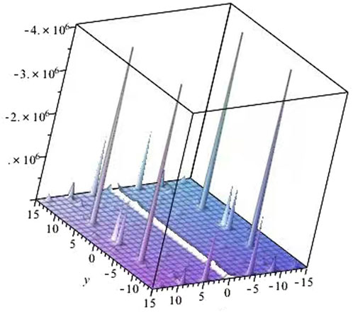
Figure 1. Solitary wave solution u10 of Equation 47, with the integration constant be one, and m 1/2 at times t = 3.14.

Figure 2

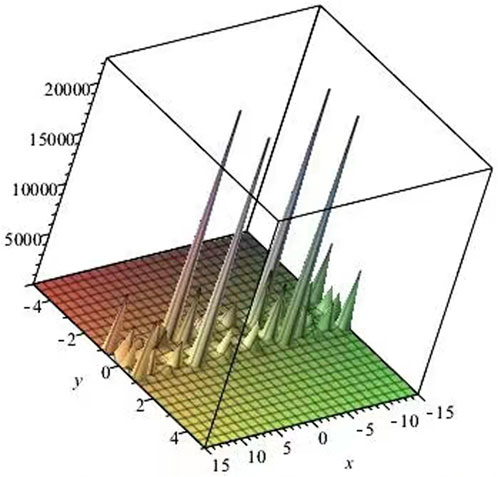
Figure 2. Solitary wave solution u15 of Equation 47, with the integration constant be one, and m = 1/2 at times t = 3.14.

5 Conclusion

In summary, the AEM is presented and applied to the generalized Schr$\ddot{\mathrm{o}}$dinger equation. As a result, several new exact solutions are obtained which include bright solitary wave solutions, dark solitary wave solutions, bell profile solitary wave solutions and Jacobian elliptic function solutions. This method is standard, direct and realized by computer mechanization, being useful for describing certain nonlinear physical phenomena as well as extended to the other nonlinear partial differential equations.

In addition, Fan and Chow [19] once applied the Bell polynomials to deduce the Darboux covariant Lax pairs and infinite conservation laws of some (2 + 1)-dimensional nonlinear evolution equations. Based on this theory, we hope investigate some corresponding properties of Equation 47 presented in the paper in future. Application of the current method to the fractional nonlinear partial differential equations is another future direction [20].

Data availability statement

The original contributions presented in the study are included in the article/supplementary material, further inquiries can be directed to the corresponding author.

Author contributions

BL: Data curation, Formal Analysis, Funding acquisition, Methodology, Resources, Software, Validation, Visualization, Writing–original draft, Writing–review and editing. FW: Conceptualization, Investigation, Supervision, Writing–original draft, Writing–review and editing.

Funding

The author(s) declare that financial support was received for the research, authorship, and/or publication of this article. The work was supported by the University Natural Science Research Project of Anhui Province (Project No. 2023AH050314) and the Horizontal Scientific Research Funds in Huaibei Normal University (No. 2024340603000006).

Conflict of interest

The authors declare that the research was conducted in the absence of any commercial or financial relationships that could be construed as a potential conflict of interest.

Generative AI statement

The author(s) declare that no Generative AI was used in the creation of this manuscript.

Publisher’s note

All claims expressed in this article are solely those of the authors and do not necessarily represent those of their affiliated organizations, or those of the publisher, the editors and the reviewers. Any product that may be evaluated in this article, or claim that may be made by its manufacturer, is not guaranteed or endorsed by the publisher.

References

1. Adeyemo O, Khalique C, Gasimov Y, Villecco F. Variational and non-variational approaches with Lie algebra of a generalized (3+1)-dimensional nonlinear potential Yu-Toda-Sasa-Fukuyama equation in Engineering and Physics. Alex Eng J (2023) 63:17–43. doi:10.1016/j.aej.2022.07.024

CrossRef Full Text | Google Scholar

2. Khalique C, Adeyemo O, Monashane M. Exact solutions, wave dynamics and conservation laws of a generalized geophysical korteweg De vries equation in ocean physics using lie ssmmetry analysis. Adv Math Models Appl (2024) 9:147–72. doi:10.62476/amma9147

CrossRef Full Text | Google Scholar

3. Ablowitz M, Clarkson P. Solitons, nonlinear evolution equations and inverse scattering. Cam-Bridge. Cambridge University Press (1991).

Google Scholar

4. Lamb GL. Analytical descriptions of ultrashort optical pulse propagation in a resonant medium. Rev Mod Phys (1971) 43:99–124. doi:10.1103/RevModPhys.43.99

CrossRef Full Text | Google Scholar

5. Zhang YF, Wang Y. A new reduction of the self-dual YangCMills equations and its applications. Z Naturforsch A (2016) 71:631–8. doi:10.1515/zna-2016-0138

CrossRef Full Text | Google Scholar

6. Zhang YF, Bai Y, Wu L. Upon generating (2+1)-dimensional dynamical systems. Int J Theor Phys (2016) 55:2837–56. doi:10.1007/s10773-016-2916-z

CrossRef Full Text | Google Scholar

7. Zhang YF, Rui WJ. A few continuous and discrete dynamical systems. Rep Math Phys (2016) 78(1):19–32. doi:10.1016/S0034-4877(16)30047-7

CrossRef Full Text | Google Scholar

8. Fan EG. Extended tanh-function method and its applications to nonlinear equations. Phys Lett A (2000) 277:212–8. doi:10.1016/S0375-9601(00)00725-8

CrossRef Full Text | Google Scholar

9. Li BC, Zhang YF. Explicit and exact travelling wave solutions for Konopelchenko-Dubrovsky equation. Chaos Soliton Fractal (2008) 38:1202–8. doi:10.1016/j.chaos.2007.01.059

CrossRef Full Text | Google Scholar

10. Dilara K, Gasimov Y, Bulut H. A sstudy on the investigation of the travelling wave solutions of the mathematical models in physics via (m + (1=g0))-expansion method. Adv Math Models Appl (2024) 9:5–13. doi:10.62476/amma9105

CrossRef Full Text | Google Scholar

11. Rabie WB, Ahmed HM, Nofal TA, Mohamed EM. Novel analytical superposed nonlinear wave structures for the eighth-order (3+1)-dimensional Kac-Wakimoto equation using improved modified extended tanh function method. AIMS Math (2024) 9:33386–400. doi:10.3934/math.20241593

CrossRef Full Text | Google Scholar

12. Li BC. New exact solutions to a category of variable-coefficient PDEs and computerized mechanization. Chin J Eng Math (2016) 33:298–308. doi:10.3969/j.issn.1005-3085.2016.03.008

CrossRef Full Text | Google Scholar

13. Sirendaoreji . A new auxiliary equation and exact travelling wave solutions of nonlinear equations. Phys Lett A, 356 (2006), 124–30. doi:10.1016/j.physleta.2006.03.034

CrossRef Full Text | Google Scholar

14. Gabriel D, Fabien N, Saidou A, Alidou M. Rogue waves dynamics of cubic-quintic nonlinear Schrodinger dinger equation with an external linear potential through a modified Noguchi electrical transmission network. Commun Nonlinear Sci (2023) 126:107479. doi:10.1016/j.cnsns.2023.107479

CrossRef Full Text | Google Scholar

15. Fan LL, Bao T. Weierstrass elliptic function solutions and degenerate solutions of a variable coefficient higher-order Schrödinger equation. Phys Scripta (2023) 98:095238. doi:10.1088/1402-4896/acec1a

CrossRef Full Text | Google Scholar

16. Jamilu S, Mayssam TS, Ali T, Hadi R, Mustafa I, Ali A. New exact solitary wave solutions of the generalized (3+1)-dimensional nonlinear wave equation in liquid with gas bubbles via extended auxiliary equation method. Opt Quant Electron (2023) 55:586. doi:10.1007/s11082-023-04870-1

CrossRef Full Text | Google Scholar

17. Wang FZ, Salama SA, Khater MA. Optical wave solutions of perturbed time-fractional nonlinear Schrodinger dinger equation. J Ocean Eng Sci Doi. doi:10.1016/j.joes.2022.03.014

CrossRef Full Text | Google Scholar

18. Zhang J, Wang FZ, Khater MA. Stable abundant computational solitary wave structures of the perturbed time-fractional NLS equation. J Ocean Eng Sci (2022). doi:10.1016/j.joes.2022.05.012

CrossRef Full Text | Google Scholar

19. Fan EG, Chow KW. Darboux covariant Lax pairs and infinite conservation laws of the (2+1)-dimensional breaking soliton equation. J Math Phys (2011) 52:1–10. doi:10.1063/1.3545804

CrossRef Full Text | Google Scholar

20. Wang FZ, Hou ER, Salama SA, Khater MA. Numerical investigation of the nonlinear fractional ostrovsky equation. Fractals (2022) 30:22401429. doi:10.1142/S0218348X22401429

CrossRef Full Text | Google Scholar